High Resolution 4-D Spectroscopy with Sparse Concentric Shell Sampling and FFT-CLEAN

SUMMARY

Recent efforts to reduce the measurement time for multidimensional NMR experiments have fostered the development of a variety of new procedures for sampling and data processing. We recently described concentric ring sampling for 3-D NMR experiments, which is superior to radial sampling as input for processing by a multidimensional discrete Fourier transform. Here, we report the extension of this approach to 4-D spectroscopy as Randomized Concentric Shell Sampling (RCSS), where sampling points for the indirect dimensions are positioned on concentric shells, and where random rotations in the angular space are used to avoid coherent artifacts. With simulations, we show that RCSS produces a very low level of artifacts, even with a very limited number of sampling points. The RCSS sampling patterns can be adapted to fine rectangular grids to permit use of the Fast Fourier Transform in data processing, without an apparent increase in the artifact level. These artifacts can be further reduced to the noise level using the iterative CLEAN algorithm developed in radioastronomy. We demonstrate these methods on the high resolution 4-D HCCH-TOCSY spectrum of protein G's B1 domain, using only 1.2% of the sampling that would be needed conventionally for this resolution. The use of a multidimensional FFT instead of the slow DFT for initial data processing and for subsequent CLEAN significantly reduces the calculation time, yielding an artifact level that is on par with the level of the true spectral noise.

INTRODUCTION

The lengthy measurement times required for multidimensional NMR spectroscopy of proteins have prompted the development of new approaches to produce high resolution spectra using shorter experiments. Instead of the conventional method of sampling on a rectangular Nyquist grid, significant attention has been devoted recently to alternative patterns for sampling the time domain (Barna and Laue 1987; Barna et al. 1987; Coggins et al. 2004, 2005; Coggins and Zhou 2006a, 2007; Ding and Gronenborn 2002; Eghbalnia et al. 2005; Freeman and Kupče 2003, 2004; Hiller et al. 2005; Kazimierczuk et al. 2006a; Kazimierczuk et al. 2006b, 2007; Kazimierczuk et al. 2008; Kim and Szyperski 2003; Koźmiński and Zhukov 2003; Kupče and Freeman 2003; Malmodin and Billeter 2005b; Marion 2006; Orekhov et al. 2001; Pannetier et al. 2007; Rovnyak et al. 2004; Schmieder et al. 1994; Simorre et al. 1994; Szyperski et al. 1993a, b; Venters et al. 2005). We previously explored radial sampling, which measures the time domain along a polar coordinate grid, yielding data that can be processed using either tomographic methods or a polar Fourier transform (Coggins et al. 2004, 2005; Coggins and Zhou 2006b, a; Kazimierczuk et al. 2006a; Kupče and Freeman 2003, 2004, 2005; Marion 2006; Venters et al. 2005; Yoon et al. 2006), or which can be analyzed as projections, as in the reduced dimensionality, GFT, HIFI, APSY and EVOCOUP methods (Ding and Gronenborn 2002; Eghbalnia et al. 2005; Hiller et al. 2005; Kim and Szyperski 2003; Malmodin and Billeter 2005a; Simorre et al. 1994; Szyperski et al. 1993a, b). We later introduced a concentric ring sampling (CRS) method, which produced fewer artifacts and better sensitivity than radial sampling for any given measurement time when used as input to a multidimensional Fourier transform (Coggins and Zhou 2007). Other groups have used purely random sampling, processing the data using the Discrete Fourier Transform (DFT) (Kazimierczuk et al. 2006b, 2007; Kazimierczuk et al. 2008; Pannetier et al. 2007), maximum entropy reconstruction (Rovnyak et al. 2004; Schmieder et al. 1994) or multidimensional decomposition (Orekhov et al. 2001; Orekhov et al. 2003). These experiments have shown that high resolution spectra can be obtained via alternative sampling in less time than would be required conventionally for the same resolution. When FT processing is used, the extra resolution is not obtained without cost: Aliasing artifacts are produced, with a form that is dictated by the sampling pattern. However, for both randomized CRS and random sampling, the artifacts assume an appearance similar to random noise, and their only consequence is an increase in the apparent noise level and reduction of the dynamic range of the spectrum.

Here we report the extension of concentric ring sampling to concentric shell sampling (CSS) for high resolution 4-D spectroscopy. Optimized sampling patterns were generated by distributing sampling points on shells, which were rotated randomly in the angular space to disrupt coherent artifacts. We show that adaptation of such sampling patterns to a sufficiently fine Cartesian grid does not significantly alter the aliasing artifact level, but enables rapid processing by the FFT. The artifact level can be reduced further by applying the CLEAN algorithm developed in the radioastronomy community (Högbom 1974). Using these methods, we were able to obtain a high resolution 4-D HCCH-TOCSY spectrum of the B1 domain of protein G (GB1) with a very low artifact level, in a significantly reduced measurement time from what would be needed conventionally.

METHODS

Placement of Sampling Points on a Shell with Uniform Distribution

In constructing sampling patterns of concentric shells, one must address the question of how points are to be arranged on each 3-D shell (representing the indirect dimensions of a 4-D experiment). For the patterns described here, uniform distributions were obtained through an iterative algorithm derived from Erber and Hockney (Erber and Hockney 1991). Sampling points were placed randomly on a shell, and their positions were allowed to evolve under a Coulombic repulsive potential until they reached a stable equilibrium.

Note that NMR sampling occurs only for positive evolution times, corresponding to a single octant out of a 3-D sphere. As described previously (Coggins and Zhou 2006a, 2007) and in a later section of this paper, during data processing we use reflection to populate other portions of the time domain with data, thereby obtaining absorptive lineshapes. To account for this during the sampling distribution calculation, each sampling point was treated as having seven duplicates in the other octants, whose positions were determined according to the rules of the reflection procedure.

The positioning algorithm, modified and optimized for the NMR sampling problem, is as follows:

1. Set a constant k to 0.002 / N, where N is the number of points to be distributed. The constant 0.002 was determined empirically.

2. Distribute N points randomly on the surface of the n-D sphere.

3. Calculate the force vector experienced by each point using Coulomb's Law. The force acting on a point i from a point j, assuming that each has an identical charge, is given by:

   $${\mathbf{F}}_{j\to i}\infty \frac{1}{r^2}{\widehat{\mathbf{r}}}_{j\to i},$$ (1)

   where r is the distance between the points and ${\widehat{\mathbf{r}}}_{j\to i}$ is the unit vector from point j to point i, and where we omit the proportionality constant, which is not needed for this non-physical situation. Since the unit vector ${\widehat{\mathbf{r}}}_{j\to i}={\mathbf{r}}_{j\to i}∕\mid {\mathbf{r}}_{j\to i}\mid$ and since $r=\mid {\mathbf{r}}_{j\to i}\mid$, the force can be written:

   $${\mathbf{F}}_{j\to i}=\frac{{\mathbf{r}}_i-{\mathbf{r}}_j}{{\mid {\mathbf{r}}_i-{\mathbf{r}}_j\mid }^3},$$ (2)

   and one obtains the following equation for computing the net force on point i:

   $${\mathbf{F}}_i=\sum _j\frac{{\mathbf{r}}_i-{\mathbf{r}}_j}{{\mid {\mathbf{r}}_i-{\mathbf{r}}_j\mid }^3},i\ne j.$$ (3)

   Equation 3 is evaluated for each of the N points, while the index of summation j includes all N points, as well as their symmetry-related duplicates.
4. Calculate an updated position for each of the N points as:

   $${\mathbf{r}}_i^{\prime }\leftarrow \frac{{\mathbf{r}}_i+k_{\mathrm{eff}}{\mathbf{F}}_i}{\mid {\mathbf{r}}_i+k_{\mathrm{eff}}{\mathbf{F}}_i\mid },$$ (4)

   where k_eff is:

   $$k_{eff}=\{\begin{array}{cc}\hfill k,\hfill & \hfill F_i<1\times {10}^7\hfill \\ \hfill \frac{k}{\sqrt{\sum _{i=1}^n{F}_i^2}},\hfill & \hfill \left(\text{otherwise}\right).\hfill \end{array}\phantom{\}}$$ (5)

   After evaluating Equation 4, the point will most likely have left the sphere. It should be projected back onto the surface of the sphere before continuing.
5. The total change in all point positions is calculated as:

   $${\Delta }_{\mathrm{pos}}=\sum _{i=1}^N\sum _{j=1}^n\mid {\mathit{r}}_{i,j}^{\prime }-{\mathit{r}}_{i,j}\mid .$$ (6)

6. If Δ_pos > 0.001, return to step there.

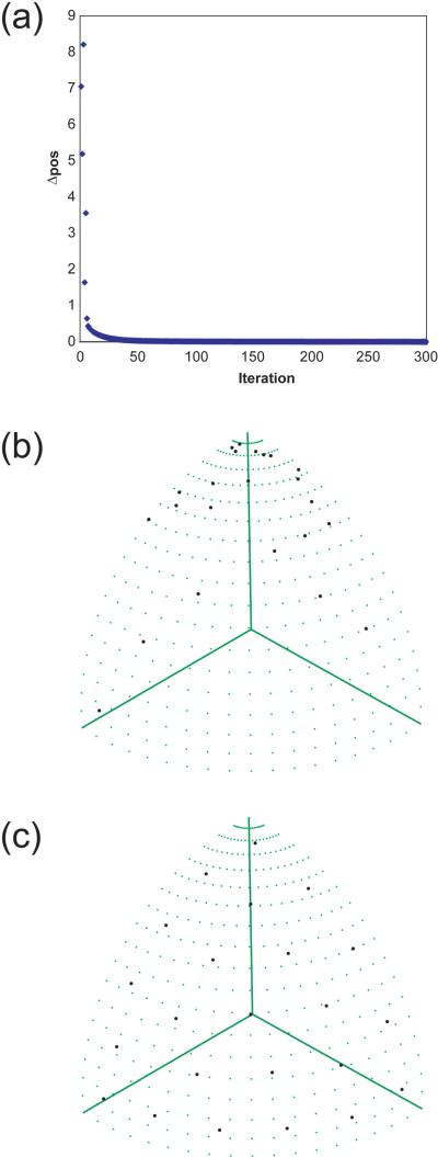
Figure 1a contains a plot of Δ_pos as a function of the iteration for a run with 23 sampling points, showing the convergence behavior of the algorithm. An example of a shell of 23 points at the start and end of the process is provided in Figures 1b and 1c.

Figure 1. Uniform Positioning of Points on a Sphere.

An example with 23 points is shown. (a) Δ_pos, the sum over all points of the distance each point was moved during an iteration, plotted as a function of the iteration number. (b) Initial random configuration of the sampling points. (c) Final configuration. The distribution of the points is roughly uniform, with roughly even spacing between them. However, there is no “perfect” configuration for 23 points, and the pattern therefore shows asymmetries and subtle variations from exact uniformity.

Randomized Concentric Shell Sampling

For non-decaying signals in 3-D NMR, we introduced the randomized linearly-increasing concentric ring sampling method, in which (1) points are placed on concentric rings with the number of points on each ring linearly proportional to its radius, and (2) the relative orientations of successive rings are randomized, preventing points from aligning on the axes to generate large coherent artifacts (Coggins and Zhou 2007). The equivalent for 4-D NMR is to sample on concentric shells, with the number of points N_j on each shell j increasing proportionally to a sampling density factor α and the square of the shell's radius r_j. Using the shell number j as a surrogate for radius we obtain:

$$N_j=\lceil \alpha {\mathit{j}}^2\rceil ,$$ (7)

where the ceiling brackets ⌈ ⌉ indicate to round up to the next higher integer. The points on each shell are distributed by the iterative positioning algorithm described above.

The continuous FT can be represented as:

$$F\left(\mathbf{X}\right)={\int }_{x}f\left(\mathbf{x}\right)e^{-2\pi i\left(\mathbf{xX}\right)}d\mathbf{X},$$ (8)

where f is the input data, F the output spectrum, x the position vector of an input point, X the position vector of an output point, and dx the differential denoting the volume of the 3-D time domain occupied by each input point. The discrete FT for CSS can be obtained easily provided that we know a discrete equivalent Δx for dx, which will serve as a weighting factor to correct for the nonuniform sampling of the time domain. By analogy to the 3-D case, we find the proper FT weighting factor Δx for any point on a shell j to be $\Delta \mathbf{x}=r_j^2∕N_j$ (or the equivalent Δx = j²/N_j). Thus the discrete Fourier Transform equation becomes:

$${\mathit{F}}_{\mathit{CSS}}\left(\mathbf{X}\right)=\sum _{j=1}^m\sum _{k=1}^{N_j}{f}_{\mathit{CSS}}\left({\mathbf{x}}_{j,k}\right){\mathit{e}}^{-2\pi i\left(\mathbf{xX}\right)}\frac{{\mathit{r}}_j^2}{{\mathit{N}}_j},$$ (9)

where m is the number of shells, and x_j,k the position vector of an input point k on shell j.

For decaying signals, one may wish to maximize sensitivity by matching the sampling distribution to the signal envelope (Barna et al. 1987; Hoch and Stern 1996). As a general-purpose approach when the signal linewidth is unknown, we propose matching the distribution to the standard cosine apodization function used in the processing of conventional NMR data, giving a modified distribution N′_j as:

$$N_j^{\prime }=\lceil \alpha {\mathit{j}}^2\cos \frac{\pi \mathit{j}}{2m}\rceil ,$$ (10)

with an FT weighting factor Δx of:

$$\Delta \mathbf{x}=\frac{{\mathit{j}}^2\cos \pi \mathit{j}∕2m}{\lceil \alpha {\mathit{j}}^2\cos \pi \mathit{j}∕2m\rceil }.$$ (11)

As shown in Figure 1c, although the positions of most sampling points on a shell as calculated by the algorithm above were randomized naturally through the random initial condition and subsequent stochastic evolution, nonetheless when equilibrium is reached the points on the edge of each shell tend to fall in regular rows, which can lead to strong artifacts at regular positions in the point response. To disrupt these coherent artifacts, we introduce randomized concentric shell sampling (RCSS): each shell computed above is rotated a random angle about each of the three axes of the experiment, in succession, with any points that pass over an edge circular-shifted back into the positive time domain octant. A similar form of randomization was recently described for radial sampling, where the blurring of radial lines produced a significant reduction in coherent artifacts (Hoch et al. 2008). The benefits of randomization in sparse, nonuniform sampling have been reviewed by Bretthorst (Bretthorst 2001).

Adaptation of Sampling Patterns to Fine Rectangular Grids

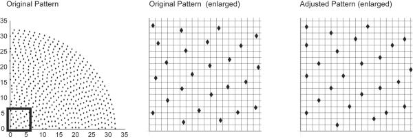
Although data from any sampling pattern can be processed with the DFT, these calculations can be exceedingly slow for high resolution 4-D spectra. In contrast, the Fast Fourier Transform (FFT) can be used to compute spectra far more efficiently than with the DFT, provided that the data points are aligned along a regular Cartesian grid. To facilitate FFT processing of concentric shell data, we evaluated the consequences of adapting RCSS sampling patterns to regular Cartesian grids. For various grid sizes, each sampling point in the pattern was replaced with its nearest neighboring grid point (Figure 2). Testing with 2-D and 3-D concentric ring patterns showed that the level of the incoherent sampling artifacts was not significantly altered by the adaptation, although at lower grid resolutions the regularity of the grid adaptation led to the appearance of additional folding artifacts along the edges of the spectrum (see the Results and Figures 4 and 5). This suggested that the FFT can be used for efficient data processing without a significant increase in the artifact level. These results are consistent with those described by Mobli et al. (Mobli et al. 2006) for the adaptation of radial sampling to fine grids prior to processing by maximum entropy reconstruction.

Figure 2. Adaptation of Sampling Patterns to a Fine Grid.

Schematic diagram showing the adjustment of points on a concentric ring sampling pattern to a fine grid. The grid spacing is approximately two times the spacing of the concentric rings.

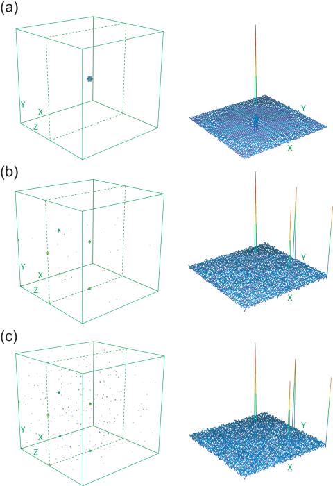
Figure 4. Point Responses for RCSS Patterns.

In each case, a 3-D contour plot is provided at left, with the lowest contour at 3% of the peak height, and additional contours at 4%, 5%, 10%, 25% and 75%. The 2-D stacked plot at right shows a cross section through the X/Y plane. Each axis has a length that is twice the intended spectral width. (a) Pattern with α = 1.0 and 32 shells, for 10,415 points. The 3-D contour plot shows no artifacts at or above 3% of the peak height. The stacked plot shows a clear zone with no artifacts extending almost the full radius of the spectrum, with artifacts appearing as random noise outside of this circle. (b) Pattern with α = 0.1, 64 shells, cosine envelope weighting and adaptation to a 64 × 64 × 64 point grid, for 3,190 sampling points. There are some artifacts at the 3% level, but almost all are lower. The stacked plot shows that these low level artifacts look like noise and cover the entirety of the spectrum, with no visible clear zone. Aliasing (folding) artifacts from the grid adaptation are visible on some edges and faces of the spectrum. (c) Pattern with α = 0.075, 64 shells, cosine envelope weighting and adaptation to a 64 × 64 × 64 point grid, for 2,399 sampling points. The results are similar to (b), but with slightly larger artifacts.

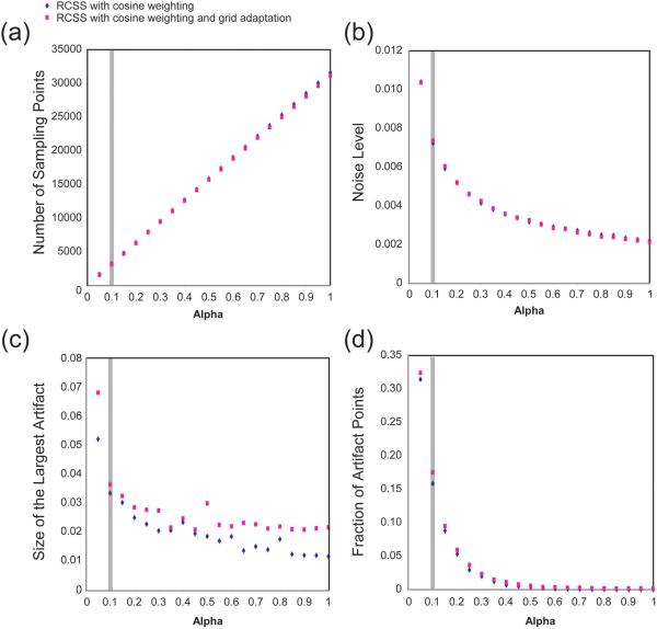
Figure 5. Properties of RCSS Sampling Patterns.

The data are measured from simulations of point responses conducted for α from 0.05 to 1.0 at 0.05 intervals. The grey bar marks the sampling used in the HCCH-TOCSY experiment. Artifacts are detected by subtracting from each point response a reference spectrum containing only the peak. (a) Number of sampling points. This quantity increases linearly with α for a given number of rings. (b) Apparent noise level, measured relative to the peak height. The noise level is calculated as described in the text. Because these data are measured from simulations, the noise level is in fact the artifact level, as there is no white noise contributing to the result. (c) Size of the largest artifact, measured relative to the peak height. Grid folding artifacts on the very edge of the spectrum are not included. (d) Fraction of artifact points. The number of points with artifacts greater than 1% is tabulated and divided by the total number of points in the spectrum.

Spectroscopy for an HCCH-TOCSY Example

A cosine-weighted RCSS sampling pattern was computed for α = 0.1 with 64 shells, giving 3,190 points. Each sampling position was then adjusted to its nearest neighboring point on a 64 × 64 × 64 grid. A 4-D triple-sensitivity-enhanced HCCH-TOCSY pulse sequence (Würtz et al. 2006) was modified to support sampling from an explicit schedule of evolution times. Data were collected using a 1.0 mM sample of uniformly ¹³C and ¹⁵N labeled GB1 at 25°C in a Varian INOVA 600 MHz spectrometer equipped with a room temperature triple-resonance probe with Z-axis gradients. The maximum evolution time for the indirectly observed proton axis was 0.0128 sec, and for each of the two carbon axes was 0.006063 sec. The spectral widths were 5,000 Hz and 10,556 Hz for proton and carbon, respectively. The total measurement time was 20 hours and 50 minutes.

FT Data Processing

Multidimensional NMR time domain data are hypercomplex. They can be processed using a true hypercomplex transform, or the hypercomplex FIDs can be taken in linear combinations to yield complex data for a complex FT. Provided that the data are sampled on a Cartesian grid, the latter approach has the advantage of permitting efficient data processing using highly optimized multidimensional FFT libraries, and it is this method that we employ. As described below, when only data for positive evolution times are used, a phase-twist lineshape is produced, but if reflections of this data into negative evolution times are added the resulting spectrum contains purely absorptive lineshapes.

For 4-D data, this process can be explained starting with a single crosspeak, which is the product of three independent signals ϕ_x, ϕ_y and ϕ_z from the three indirectly observed nuclei that are correlated in the peak. Note that each of these signals is itself a complex phasor

$${\varphi }_x\left(\mathit{x}\right)={\mathit{e}}^{i{w}_{x}x},{\varphi }_y\left(\mathit{y}\right)={\mathit{e}}^{i{w}_{y}y},{\varphi }_z\left(\mathit{z}\right)={\mathit{e}}^{i{w}_{z}z},$$ (12)

where the coordinates x, y and z represent the evolution times of the three signals and ω_x, ω_y and ω_z the frequencies. A complex-valued time domain would require phase-modulated signals of the form:

$$\begin{array}{cc}\hfill {\varphi }_{\mathit{xyz}}(x,y,z)& ={\varphi }_x\left(x\right){\varphi }_y\left(y\right){\varphi }_z\left(z\right)\hfill \\ \hfill & =e^{i{w}_{x}x}{e}^{i{w}_{y}y}{e}^{i{w}_{z}z}=e^{i(w_{x}x+w_{y}y+w_{z}z)}\hfill \\ \hfill & =(cx+isx)(cy+isy)(cz+isz)\hfill \\ \hfill & =\left[\left(cx\right)\left(cy\right)\left(cz\right)-\left(cx\right)\left(sy\right)\left(sz\right)-\left(sx\right)\left(cy\right)\left(sz\right)-\left(sx\right)\left(sy\right)\left(cz\right)\right]+i\left[\left(cx\right)\left(cy\right)\left(sz\right)+\left(cx\right)\left(sy\right)\left(cz\right)+\left(sx\right)\left(cy\right)\left(cz\right)+\left(sx\right)\left(sy\right)\left(sz\right)\right],\hfill \end{array}$$ (13)

where we abbreviate cos as “c,” sin as “s,” and arguments of the form ω_xx as “x.” The hypercomplex data acquisition gives eight amplitude-modulated FIDs:

$$\begin{array}{c}\hfill I_1=\left(cx\right)\left(cy\right)\left(cz\right)I_5=\left(sx\right)\left(cy\right)\left(cz\right)\hfill \\ \hfill I_2=\left(cx\right)\left(cy\right)\left(sz\right)I_6=\left(sx\right)\left(cy\right)\left(sz\right)\hfill \\ \hfill I_3=\left(cx\right)\left(sy\right)\left(cz\right)I_7=\left(sx\right)\left(sy\right)\left(cz\right)\hfill \\ \hfill I_4=\left(cx\right)\left(sy\right)\left(sz\right)I_8=\left(sx\right)\left(sy\right)\left(sz\right),\hfill \end{array}$$ (14)

which can be combined directly:

$$f_{+x+y+z}(x,y,z)=(I_1-I_4-I_6-I_7)+i(I_2+I_3+I_5-I_8),$$ (15)

to yield the desired phase-modulated form of data from Equation 13. Considering that the signals in a hypothetical region of the time domain with negative evolution times would simply have the sign of precession reversed for one or more of the signals ϕ_x, ϕ_y and ϕ_z, one finds the related combinations for populating three other octants of the 3-D indirectly observed space to be:

$$\begin{array}{c}\hfill f_{-x+y+z}(x,y,z)=(I_1-I_4+I_6+I_7)+i(I_2+I_3-I_5+I_8)\hfill \\ \hfill f_{+x-y+z}(x,y,z)=(I_1+I_4-I_6+I_7)+i(I_2-I_3+I_5+I_8)\hfill \\ \hfill f_{-x-y+z}(x,y,z)=(I_1+I_4+I_6-I_7)+i(I_2-I_3-I_5-I_8).\hfill \end{array}$$ (16)

Because the three dimensions are independent, the complex FT Φ of the 3-D signal ϕ can be decomposed as:

$$\Phi (X,Y,Z)={\Phi }_X\left(X\right){\Phi }_Y\left(Y\right){\Phi }_Z\left(Z\right).$$ (17)

If only positive evolution times are used, each 1-D signal has a transform:

$${\Phi }_{+X}\left(X\right)=A\left(X\right)+iD\left(X\right),$$ (18)

where A(X) is the absorptive lineshape and D(X) is the dispersive lineshape. For the product of three such signals, the FT would have a “phase-twist” multidimensional lineshape:

$$\mathrm{Re}\left[{\Phi }_{+x+y+z}(X,Y,Z)\right]=A\left(X\right)A\left(Y\right)A\left(Z\right)-A\left(X\right)D\left(Y\right)D\left(Z\right)-D\left(X\right)A\left(Y\right)D\left(Z\right)-D\left(X\right)D\left(Y\right)A\left(Z\right).$$ (19)

By combining data from four octants, the dispersive elements are eliminated:

$$\begin{array}{cc}\hfill \mathrm{Re}\left[{\Phi }_{\pm x\pm y\pm z}(X,Y,Z)\right]& =(AAA-ADD-DAD-DDA)\hfill \\ \hfill & +(AAA-ADD+DAD+DDA)\hfill \\ \hfill & +(AAA+ADD-DAD+DDA)\hfill \\ \hfill & +(AAA+ADD+DAD-DDA)\hfill \\ \hfill & =4AAA,\hfill \end{array}$$ (20)

to give a purely absorptive lineshape. In practice, the conversion from hypercomplex to complex data and the preparation of reflected data for negative evolution times are almost identical to the “separation of intermodulated projection” step in projection-reconstruction NMR, or to the G-matrix step in GFT NMR, and can be carried out conveniently using the PRSP program (Coggins and Zhou 2006b).

After this preparatory step, one has four time domain data files containing f_+x,+y,+z, f_+x-y+z, f_-x+y+z and f_-x-y+z at the specific locations measured according to the grid-adapted sampling schedule. For the example, we processed the directly-observed dimension of each of these files using NMRPipe (Delaglio et al. 1995) according to standard methods. The FT of the remaining three dimensions was carried out in a custom C++ program operating on all four inputs. For each 3-D cube at a given position on the directly observed axis, a 128 × 128 × 128 point matrix was constructed and populated with the input data, with a zero value for all grid points that were not sampled. The matrix size was twice the size of the grid used in the creation of the sampling pattern to accommodate the reflections in x and y; the extra points in the z axis are not necessary but serve as zero-filling to improve the digital resolution. The positive and (reflected) negative time domain data are rearranged when copied to and from the FFT matrix as described in standard sources (Press et al. 1992). The SCITBX library (Computational Crystallography Initiative, Lawrence Berkeley National Laboratory, Berkeley, CA) was used for FFTs.

CLEAN Processing

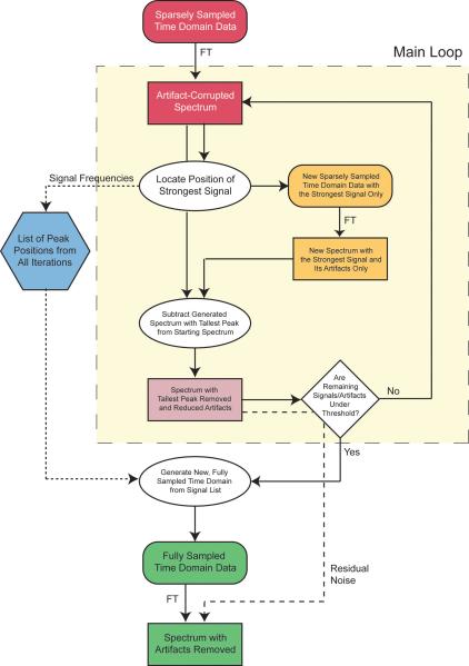
The CLEAN algorithm (Högbom 1974) is an iterative process built on a cycle of (1) finding the strongest peak in a spectrum, (2) generating a replica, called a component, of the peak and its artifact pattern based on knowledge of the sampling schedule, and (3) subtracting the component with the artifact pattern and peak, leaving a spectrum with one less peak and a reduced artifact level (Figure 3). This process is repeated until a threshold is reached, at which point artifact-free signals at the original peak positions are added back. Our implementation of CLEAN is derived from the standard versions used in the radioastronomy and imaging fields, with some modifications. In particular, instead of using a simple threshold as the criterion for stopping the calculation, we have developed a more elaborate method that is able to detect when the algorithm is no longer successfully reducing the artifact level. Although CLEAN can be carried out with fitted lineshapes, we find it more straightforward and robust to use nondecaying components, which has the effect of decomposing each peak into discrete points. Thus for each iteration we simply locate the strongest data point in the spectrum and use a nondecaying signal at that position as the input for the generation of the peak and artifact pattern (component) to subtract.

Figure 3.

Flow Chart for CLEAN

The details of our implementation, as applied individually to each 3-D cube from a 4- D spectrum, are as follows:

1. Initialization: Compute the FFT Φ of the input data ϕ. This will be considered iteration i = 0, and thus spectrum Φ₀.

2. Main Loop: Identify the tallest point in the spectrum Φ_i for this iteration i, the frequencies ω_x,i, ω_y,i and ω_z,i corresponding to this point, and its relative intensity I_i. Evaluate the two stopping criteria: (a) Calculate the noise level n_i as described below. Compute the running average of the noise level over the previous 15 iterations. If the 15-iteration running average of the noise level has been no more than τn_i for the previous 25 iterations, where τ is a threshold parameter, stop and go to step seven. (b) If the intensity I_i is no more than 5n_i, stop and go to step seven. Otherwise store ω_x,i, ω_y,i ω_z,i and I_i and continue with step three.

3. Generate a new set of sparsely sampled input data ψ_i according to the known sampling pattern, containing a single nondecaying signal with the frequencies ω_x,i, ω_y,i and ω_z,i identified in step two. This is the component for this iteration.

4. Compute the FFT Ψ_i of the component ψ_i (N.B. this is effectively the point response of the sampling pattern, except that it is shifted in position so that it is centered on the location of the tallest point in step two).

5. Adjust the scale of the new component spectrum Ψ_i such that the height of the peak is gI_i, where g is the user-specified loop gain parameter, in the range 0 < g < 1.

6. Subtract Ψ_i from Φ_i to give a new spectrum Φ_i+1. This will serve as the input for the next iteration i + 1. Go back to step 2.

7. Final Processing: Generate a new time domain ϕ_CLEAN with full, rather than sparse, sampling. Populate this ϕ_CLEAN with artificially generated signals at the frequencies ω_x,i, ω_y,i and ω_z,i and intensities I_i recorded in the previous iterations.

8. Compute the FFT of φ_CLEAN to give a new spectrum Φ_CLEAN. Scale this spectrum so that its tallest peak matches the starting intensity I₀. Add the residual spectrum Φ_i from the last iteration. This spectrum Φ_CLEAN is the final result.

The two criteria that we use to stop the CLEAN calculation differ from some other implementations in that they are not based on a fixed, absolute threshold, but rather are adjusted dynamically for the case at hand to detect the point at which further calculation is no longer beneficial. This automatic selection of a termination threshold is especially advantageous for sparsely sampled NMR data, where the artifact level varies enormously between different 3-D cubes of the spectrum, being proportional to the peak heights and additive with more peaks. The first criterion (step 2a) stops the calculation when the noise level has stabilized. The noise level is smoothed using an average over 15 iterations. The calculation is stopped when the smoothed noise level is within a user-specified threshold τ of the current value, typically 5%, for 25 consecutive iterations (i.e. if τ = 5%, then the condition is n_j ≤ 1.05n_i for all j in the range i - 25 ≤ j < i). The use of a 15-iteration running average is important for filtering out fluctuations from iteration to iteration that are not significant in evaluating the progress of the calculation. The second criterion (step 2b), which stops the calculation when the tallest value is within five multiples of the noise standard deviation, serves to detect cubes that do not contain peaks, or that contain only small peaks, and provides an appropriate termination for those cases in which the apparent noise level does not stabilize quickly. For both criteria, it is important to have an accurate measurement of the noise level. We use a procedure adapted from Delaglio et al. (Delaglio et al. 1995) to determine the noise standard deviation without skewing of the parameters by the peaks, wherein:

1. Twenty-four 1-D vectors are selected from the 3-D cube spaced throughout the cube and running in different directions.

2. The deviations of the data values on each vector are sorted.

3. The standard deviation of each vector is inferred from the size of the deviation at the 30% percentile from the bottom of the distribution.

4. The median of the standard deviations determined from the different vectors is taken.

The components ψ_i generated in step four of the CLEAN algorithm are not given a linewidth: We found that better results are obtained if the signals are broken down into almost infinitely sharp components corresponding to the individual points of the grid, a decomposition that is permissible due to the linearity of the FT (and which is essentially the same as the decomposition inherent in discrete Fourier analysis). This method removes the need for explicit assumptions about lineshape and a fitting procedure to match the signals to the model. Our simulations additionally suggest that decomposition into a superposition of extremely sharp components improves the results for large or overlapping peaks. It would seem appropriate to apply apodization in step four to match whatever apodization the user may have selected in step one. For the example described in this article, however, such apodization is carried out rather through cosine weighting in the sampling pattern itself, and no supplemental apodization is needed in the calculation of the spectrum. An appropriate cosine window function is used in step eight to match the weighting profile used in the sampling pattern.

For the HCCH-TOCSY experiment, CLEAN was applied with a loop gain setting g of 30%, a stopping threshold τ of 5%, and a 500 iteration maximum run for each cube.

Software Availability

The custom C++ programs described above are available upon request from the authors.

RESULTS

Characteristics of Concentric Shell Sampling

As with concentric ring sampling for 3- D spectroscopy (Coggins and Zhou 2007), the RCSS method for concentric shell sampling of 4-D spectra produces an artifact-free “clear zone” around each peak, with artifacts that appear as random noise beginning just outside the clear zone. Figure 4a shows a 3-D contour plot of, and 2-D X/Y cross sections through, a simulated point response for an RCSS pattern with α = 1.0 and 32 rings (10,415 sampling points).

Unfortunately, obtaining a substantial clear zone requires on the order of 25-50% of the number of sampling points that would be needed conventionally at the same resolution (31.8% for the example in the preceeding paragraph), and is of relatively little practical value for high resolution 4-D spectroscopy.

More useful examples would be the grid-adapted, cosine-weighted 64 ring RCSS patterns with α = 0.1 and α = 0.075 (3,190 and 2,399 sampling points, respectively), which would require only 1.2% and 0.9%, respectively, of the conventional sampling needed for a spectrum with 64 points in each indirect dimension. Figures 4b and 4c show 3-D contour plots and 2-D sections through the point response for these patterns. No clear zone is apparent. Artifacts appear like random noise, almost entirely at less than 2% of the peak height. One can also see on the very edges of the spectrum the folding artifacts from the grid adaptation.

To provide a more quantitative evaluation of the characteristics of the sampling, we calculated the point responses expected for RCSS with cosine weighting and RCSS with cosine weighting and adaptation to a 64 × 64 × 64 point grid. For each of these two configurations, we tested 64 ring patterns with values of α from 0.05 to 1.00, in increments of 0.05. The apparent noise level, the maximum artifact height and the portion of the spectrum containing artifacts above 1% of peak height were measured. These results are plotted in Figure 5 relative to the height of the peak or the total number of points in the spectrum, with a gray bar indicating the degree of sampling used for the HCCH-TOCSY spectrum, as applicable. These graphs show that the average size, maximum size and number of artifacts all decrease as α is increased. They also show that the grid adaptation has minimal impact on the results, with no effect on the noise level or number of artifacts, and only a slight increase in the size of the largest artifact.

Application of RCSS Data Collection and FT Processing to an HCCH-TOCSY Spectrum

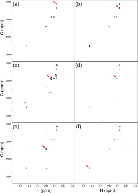
We applied RCSS to the 4-D HCCH-TOCSY spectrum of GB1. As a typical example of the results obtained, Figure 6 shows Ile6. The panels of this figure show different F1/F2 planes from the 4-D spectrum, with each plane taken at the F3/F4 position corresponding to one of the CH correlations from the spin system. Depending on the transfer efficiency one finds most or all of the spin system replicated at each of these positions, with some planes showing overlap with other spin systems. For each plane, the Ile crosspeaks are seen well above the artifact level, and with no apparent distortion.

Figure 6. Experimental Results for RCSS on an HCCH-TOCSY Spectrum.

As an example, six different views of the Ile6 spin system are shown. In each case, the F1/F2 (h/c) correlations are shown at the F3/F4 (C/H) position in the 4-D spectrum corresponding to one of the crosspeaks (indicated by arrows). (a) The h/c plane at the H/C position H = 0.73 ppm, C = 12.6 ppm of Ile6 H^δ1/C^δ1. (b) H=0.78 ppm, C = 16.9 ppm for Ile6 H^γ2/C^γ2. (c) H = 1.35 ppm, C = 27.1 ppm for Ile6 H^γ12/C^γ1. (d) H = 1.05 ppm, C = 27.1 ppm for Ile6 H^γ13/C^γ1. (e) H = 1.96 ppm, C = 37.9 ppm for Ile6 H^β/C^β. (f) H = 4.27 ppm, C = 60.1 ppm for H^α/C^α.

CLEAN

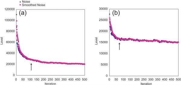
Figure 7 shows the progress of a typical CLEAN calculation from the HCCH-TOCSY spectrum, specifically for the δ1 and γ2 methyl proton correlations of the Ile example from Figure 6, as measured by the noise level after each iteration. For cubes with multiple crosspeaks, one finds that the noise level declines rapidly in the first 50-100 iterations, completing 90% or more of the potential improvement. Depending on the case, it may have reached the level of the white noise, in which case no further improvement is possible, or it may show an additional but much slower improvement of up to 10% more over several hundred more iterations. It was on the basis of these curves that we developed criteria for discontinuing a calculation once the noise level has stabilized or once it has entered the slow phase of improvement. The graphs in Figure 7 are annotated to indicate when the noise stability criterion would have become active for a 5% threshold τ. Using these criteria, the HCCH-TOCSY experiment required, on average, 63 iterations per cube. The apparent noise level was reduced 44% on average and as much as 78% for some cubes. With 127 cubes, the calculation was completed in 110 minutes on a quad-core 2.4 GHz Intel computer. If every cube were calculated for 500 iterations, the apparent noise would be reduced an additional ~5%.

Figure 7. CLEAN Progress.

The graphs show the estimated noise level over the course of a CLEAN run for two 3-D cubes from the HCCH-TOCSY. The smoothed noise is computed with a 15-iteration window. The arrow indicates the point at which a 5% noise stabilization cutoff would be activated to stop the calculation. (a) H = 0.73 ppm, for Ile6 H^δ1. The stopping point is 111 iterations. (b) H = 0.78 ppm, for Ile6 H^γ2. The stopping point is 63 iterations.

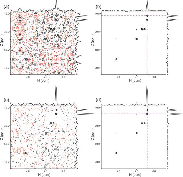
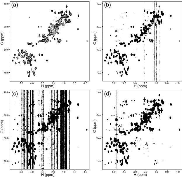
Results with and without CLEAN for the two Ile examples are provided in Figure 8, where the same contour level is used for each comparison. Figure 9 shows the consequences of CLEAN processing on the spectrum as a whole, as illustrated by the projection of the spectrum onto the H/C HSQC plane. The artifact level for the whole spectrum is significantly reduced via CLEAN, with the average apparent noise for the whole spectrum decreasing from 2.4x the white noise level (as measured on cubes with no peaks) to 1.4x.

Figure 8. Comparison of Results with and without CLEAN.

(a) The plane from the 4-D HCCH-TOCSY at H = 0.73 ppm, C = 12.6 ppm (Ile6 H^δ1/C^δ1), for processing with the FT alone. (b) The same plane as in (a) after processing with CLEAN, plotted at the same contour level. The calculation was stopped automatically under the 5% noise stabilization criteria. (c) The plane at H=0.78 ppm, C = 16.9 ppm (Ile6 H^γ2/C^γ2), without CLEAN and (d) with CLEAN.

Figure 9. Results for the Full HCCH-TOCSY Spectrum.

(a) The H/C HSQC spectrum of GB1. (b) A projection of the 4-D RCSS HCCH-TOCSY onto the H/C plane. The vertical stripes are the result of cubes that have an especially high level of artifacts. (c) The same as (b), but plotted at a contour level that is 55% lower. (d) The same as (c), at the same contour level, but after CLEAN.

DISCUSSION

Sparse Sampling

Reducing the required measurement time for high resolution 4-D experiments would have many potential practical benefits for NMR studies of proteins, particularly with respect to studies of large proteins, where signal overlap is a severe problem. Although sensitivity considerations can be critical for such cases, and may necessitate a very significant minimal measuring time on the order of days, it is important to remember that the ideal 4-D experiment for many applications would have a much higher resolution than is common today, requiring much longer experiments than are practical or than are required for sensitivity. One can thus fairly say that such high-resolution 4-D experiments are sampling-limited, and would benefit from new sampling procedures.

We demonstrated some of the potential benefits of these methods previously with a high resolution 4-D methyl-amide NOESY experiment, which used radial sampling at 4% of the conventional time requirement, and which was processed using tomographic reconstruction (Coggins et al. 2005). RCSS provides an advantage over radial sampling by achieving a higher resolution spectrum, with fewer and smaller artifacts, for significantly less sampling points than even radial sampling. The capabilities of the method are particularly clear for the example case, a triple-senstivity-enhanced HCCH-TOCSY from the small protein GB1, which was recorded in 20 hours at a resolution that would have required 8 to 70 days for conventional sampling, depending on whether or not one used two-fold linear prediction in the indirect dimensions. With FT processing alone, the average artifact level was approximately 5% of the height of the strongest peak, which is adequate for the interpretation of a TOCSY spectrum.

A number of other sampling methods have been suggested recently (Barna and Laue 1987; Barna et al. 1987; Coggins and Zhou 2006a, 2007; Freeman and Kupče 2004; Kazimierczuk et al. 2006a; Kazimierczuk et al. 2006b, 2007; Kazimierczuk et al. 2008; Marion 2006; Pannetier et al. 2007; Rovnyak et al. 2004; Schmieder et al. 1994), and the merits of these sampling patterns remain to be evaluated systematically. However, given the significantly varied requirements of different applications and the many spectroscopic conditions encountered it is unlikely that any particular method will prove superior in all cases. For example, for dipolar coupling applications the accuracy of the peak positions is most important, whereas for NOESY the sensitivity and the linearity of response are most important, and the optimum sampling may yet be different depending on whether or not the signals are decaying. The particular trade-offs of each sampling method will have to be considered relative to the application before the best answers will emerge.

CLEAN

CLEAN is very popular in several other fields, but has seen only limited application in NMR (Barna et al. 1988; Davies et al. 1988; Kazimierczuk et al. 2007; Keeler 1984; Kupče and Freeman 2005; Shaka et al. 1984). Earlier studies attempted to apply it for the removal of unwanted dispersive signals (Shaka et al. 1984), elimination of truncation artifacts (Keeler 1984), or enhancement of spectral resolution for 1-D and 2-D studies of small molecules (Barna et al. 1988; Davies et al. 1988). Resolution enhancement of fine structure is a challenging problem for CLEAN, requiring assumptions about lineshape, accurate fitting of model parameters, very small loop gain settings and correspondingly long calculations, and can lead to false peak splittings in some cases. By contrast, for artifact suppression with sparse signals in higher dimensions, a loop gain setting of 30% can be used with no apparent difficulty, and no explicit assumptions about lineshape are needed.

Recently, a variant on CLEAN was introduced by Kupče and Freeman for use with artifact suppression in (3,2)-D radial sampling (Kupče and Freeman 2005). This method is tailored specifically for the context of reconstructing a spectrum from projections. For each iteration, a spectrum is reconstructed from the projections and the tallest signal is determined; however, in the next step the components are calculated for and subtracted from the projections themselves. Kazimierczuk et al. have also introduced a version of CLEAN (Kazimierczuk et al. 2007), in which all peaks are picked by the user and parameters extracted by a lineshape fitting algorithm. A single component is then generated containing the signals and artifacts for all of these peaks, and the single component is subtracted in one step. The principal advantage of the classic iterative CLEAN algorithm over this latter method is that the classic CLEAN is able to decouple the artifactural interference of signals and uncover low level peaks that are obscured by artifacts from the larger peaks. The newly identified lower-level peaks and their associated artifacts are then further removed by the iterative process, which should yield better artifact suppression and a higher dynamic range.

The adaptation of the sampling patterns to fine grids is essential to facilitating the application of CLEAN to sparsely sampled data. The time required for the FFT of a cube from the HCCH-TOCSY spectrum is a tiny fraction of that needed for the DFT, making it possible to achieve the complete CLEAN processing of a single cube in a couple of minutes on a modern desktop workstation, and an entire spectrum within hours.

For practical application of these methods, the first consideration would always be sensitivity: The number of sampling points must be large enough to provide sufficient signal accumulation to observe all of the peaks. After also estimating the dynamic range needed, one can then use the curves plotted in Figure 5 and the statistical measures cited in the Results section to determine the appropriate sampling parameters.

CONCLUSIONS

We have introduced a new sampling method for 4-D spectroscopy called RCSS that uses concentric shells of sampling points. Simulations show that RCSS patterns with very small numbers of sampling points give very low artifact levels, even at high resolution, when processed using the FT. Adaptation of the RCSS pattern to a fine Cartesian grid does not significantly increase the aliasing artifact level, but enables efficient data processing with the FFT. The method was used to collect a very high resolution 4-D HCCH-TOCSY spectrum of GB1 with only 1.2% of the sampling points needed conventionally. To reduce the artifact level further, we used the CLEAN procedure from radioastronomy to take the artifact level on average from 2.4x the white noise level to 1.4x, and in some cases on to the true noise level. The complete processing of a high-resolution 4-D spectrum (with 128 points per indirect axis) takes less than two hours. The significant reduction of data collection time coupled with efficient data processing renders this approach highly attractive for obtaining high resolution 4-D spectra for biomolecular NMR studies.

REFERENCES

- Barna JCJ, Laue ED. Conventional and exponential sampling for 2D NMR experiments with application to a 2D NMR spectrum of a protein. J Magn Reson. 1987;75:384–389. [Google Scholar]
- Barna JCJ, Laue ED, Mayger MR, Skilling J, Worrall SJP. Exponential sampling, an alternative method for sampling in two-dimensional NMR experiments. J Magn Reson. 1987;73:69–77. [Google Scholar]
- Barna JCJ, Tan SM, Laue ED. Use of CLEAN in conjunction with selective data sampling for 2D NMR experiments. J Magn Reson. 1988;78:327–332. [Google Scholar]
- Bretthorst GL. Nonuniform sampling: bandwidth and aliasing. In: Rychert JT, Erickson GJ, Smith CR, editors. Bayesian inference and maximum entropy methods in science and engineering. American Institute of Physics; 2001. pp. 1–28. [Google Scholar]
- Coggins BE, Venters RA, Zhou P. Generalized reconstruction of n-D NMR spectra from multiple projections: application to the 5-D HACACONH spectrum of protein G B1 domain. J Am Chem Soc. 2004;126:1000–1001. doi: 10.1021/ja039430q. [DOI] [PubMed] [Google Scholar]
- Coggins BE, Venters RA, Zhou P. Filtered backprojection for the reconstruction of a high-resolution (4,2)D CH3-NH NOESY spectrum on a 29 kDa protein. J Am Chem Soc. 2005;127:11562–11563. doi: 10.1021/ja053110k. [DOI] [PubMed] [Google Scholar]
- Coggins BE, Zhou P. Polar Fourier transforms of radially sampled NMR data. J Magn Reson. 2006a;182:84–95. doi: 10.1016/j.jmr.2006.06.016. [DOI] [PubMed] [Google Scholar]
- Coggins BE, Zhou P. PR-CALC: a program for the reconstruction of NMR spectra from projections. J Biomol NMR. 2006b;34:179–195. doi: 10.1007/s10858-006-0020-z. [DOI] [PMC free article] [PubMed] [Google Scholar]
- Coggins BE, Zhou P. Sampling of the NMR time domain along concentric rings. J Magn Reson. 2007;184:219–233. doi: 10.1016/j.jmr.2006.10.002. [DOI] [PMC free article] [PubMed] [Google Scholar]
- Davies SJ, Bauer C, Hore PJ, Freeman R. Resolution enhancement by nonlinear data processing. “HOGWASH” and the maximum entropy method. J Magn Reson. 1988;76:476–493. [Google Scholar]
- Delaglio F, Grzesiek S, Vuister GW, Zhu G, Pfeifer J, Bax A. NMRPipe: a multidimensional spectral processing system based on UNIX pipes. J Biomol NMR. 1995;6:277–293. doi: 10.1007/BF00197809. [DOI] [PubMed] [Google Scholar]
- Ding K, Gronenborn AM. Novel 2D triple-resonance NMR experiments for sequential resonance assignments of proteins. J Magn Reson. 2002;156:262–268. doi: 10.1006/jmre.2002.2537. [DOI] [PubMed] [Google Scholar]
- Eghbalnia HR, Bahrami A, Tonelli M, Hallenga K, Markley JL. High-resolution iterative frequency identification for NMR as a general strategy for multidimensional data collection. J Am Chem Soc. 2005;127:12528–12536. doi: 10.1021/ja052120i. [DOI] [PMC free article] [PubMed] [Google Scholar]
- Erber T, Hockney GM. Equilibrium configurations of N equal charges on a sphere. J Phys A: Math Gen. 1991;24:L1369–L1377. [Google Scholar]
- Freeman R, Kupče E. New methods for fast multidimensional NMR. J Biomol NMR. 2003;27:101–113. doi: 10.1023/a:1024960302926. [DOI] [PubMed] [Google Scholar]
- Freeman R, Kupče E. Distant echoes of the accordion: reduced dimensionality, GFT-NMR, and projection-reconstruction of multidimensional spectra. Concepts in Magnetic Resonance. 2004;23A:63–75. [Google Scholar]
- Hiller S, Fiorito F, Wüthrich K, Wider G. Automated projection spectroscopy (APSY) Proc Natl Acad Sci U S A. 2005;102:10876–10881. doi: 10.1073/pnas.0504818102. [DOI] [PMC free article] [PubMed] [Google Scholar]
- Hoch JC, Stern AS. NMR data processing. Wiley-Liss; New York: 1996. [Google Scholar]
- Hoch JC, Maciejewski MW, Filipovic B. Randomization improves sparse sampling in multidimensional NMR. J Magn Reson. 2008;193:317–320. doi: 10.1016/j.jmr.2008.05.011. [DOI] [PMC free article] [PubMed] [Google Scholar]
- Högbom JA. Aperture synthesis with a non-regular distribution of interferometer baselines. Astron Astrophys Suppl. 1974;15:417–426. [Google Scholar]
- Kazimierczuk K, Koźmiński W, Zhukov I. Two-dimensional Fourier transform of arbitrarily sampled NMR data sets. J Magn Reson. 2006a;179:323–328. doi: 10.1016/j.jmr.2006.02.001. [DOI] [PubMed] [Google Scholar]
- Kazimierczuk K, Zawadzka A, Koźmiński W, Zhukov I. Random sampling of evolution time space and Fourier transform processing. J Biomol NMR. 2006b;36:157–168. doi: 10.1007/s10858-006-9077-y. [DOI] [PubMed] [Google Scholar]
- Kazimierczuk K, Zawadzka A, Koźmiński W, Zhukov I. Lineshapes and artifacts in Multidimensional Fourier Transform of arbitrary sampled NMR data sets. J Magn Reso. 2007;188:344–356. doi: 10.1016/j.jmr.2007.08.005. [DOI] [PubMed] [Google Scholar]
- Kazimierczuk K, Zawadzka A, Koźmiński W. Optimization of random time domain sampling in multidimensional NMR. J Magn Reson. 2008;192:123–130. doi: 10.1016/j.jmr.2008.02.003. [DOI] [PubMed] [Google Scholar]
- Keeler J. Elimination of truncation artifacts from NMR spectra. Application to carbon-13 multiplicity determination by two-dimensional spectroscopy. J Magn Reson. 1984;56:463–470. [Google Scholar]
- Kim S, Szyperski T. GFT NMR, a new approach to rapidly obtain precise high-dimensional NMR spectral information. J Am Chem Soc. 2003;125:1385–1393. doi: 10.1021/ja028197d. [DOI] [PubMed] [Google Scholar]
- Koźmiński W, Zhukov I. Multiple quadrature detection in reduced dimensionality experiments. J Biomol NMR. 2003;26:157–166. doi: 10.1023/a:1023550224391. [DOI] [PubMed] [Google Scholar]
- Kupče E, Freeman R. Reconstruction of the three-dimensional NMR spectrum of a protein from a set of plane projections. J Biomol NMR. 2003;27:383–387. doi: 10.1023/a:1025819517642. [DOI] [PubMed] [Google Scholar]
- Kupče E, Freeman R. The Radon transform: a new scheme for fast multidimensional NMR. Concepts in Magnetic Resonance. 2004;22A:4–11. [Google Scholar]
- Kupče E, Freeman R. Fast multidimensional NMR: radial sampling of evolution space. J Magn Reson. 2005;173:317–321. doi: 10.1016/j.jmr.2004.12.004. [DOI] [PubMed] [Google Scholar]
- Malmodin D, Billeter M. Signal identification in NMR spectra with coupled evolution periods. J Magn Reson. 2005a;176:47–53. doi: 10.1016/j.jmr.2005.05.020. [DOI] [PubMed] [Google Scholar]
- Malmodin D, Billeter M. Multiway decomposition of NMR spectra with coupled evolution periods. J Am Chem Soc. 2005b;127:13486–13487. doi: 10.1021/ja0545822. [DOI] [PubMed] [Google Scholar]
- Marion D. Processing of ND NMR spectra sampled in polar coordinates: a simple Fourier transform instead of a reconstruction. J Biomol NMR. 2006;36:45–54. doi: 10.1007/s10858-006-9066-1. [DOI] [PubMed] [Google Scholar]
- Mobli M, Stern AS, Hoch JC. Spectral reconstruction methods in fast NMR: reduced dimensionality, random sampling and maximum entropy. J Magn Reson. 2006;182:96–105. doi: 10.1016/j.jmr.2006.06.007. [DOI] [PubMed] [Google Scholar]
- Orekhov VY, Ibraghimov IV, Billeter M. MUNIN: a new approach to multidimensional NMR spectra interpretation. J Biomol NMR. 2001;20:49–60. doi: 10.1023/a:1011234126930. [DOI] [PubMed] [Google Scholar]
- Orekhov VY, Ibraghimov I, Billeter M. Optimizing resolution in multidimensional NMR by three-way decomposition. J Biomol NMR. 2003;27:165–173. doi: 10.1023/a:1024944720653. [DOI] [PubMed] [Google Scholar]
- Pannetier N, Houben K, Blanchard L, Marion D. Optimized 3D-NMR sampling for resonance assignment of partially unfolded proteins. J Magn Reson. 2007;186:142–149. doi: 10.1016/j.jmr.2007.01.013. [DOI] [PubMed] [Google Scholar]
- Press WH, Flannery BP, Teukolsky SA, Vetterling WT. Numerical recipes in C: the art of scientific computing. Cambridge University Press; Cambridge: 1992. [Google Scholar]
- Rovnyak D, Frueh DP, Sastry M, Sun ZY, Stern AS, Hoch JC, Wagner G. Accelerated acquisition of high resolution triple-resonance spectra using non-uniform sampling and maximum entropy reconstruction. J Magn Reson. 2004;170:15–21. doi: 10.1016/j.jmr.2004.05.016. [DOI] [PubMed] [Google Scholar]
- Schmieder P, Stern AS, Wagner G, Hoch JC. Improved resolution in triple-resonance specra by nonlinear sampling in the constant-time domain. J Biomol NMR. 1994;4:483–490. doi: 10.1007/BF00156615. [DOI] [PubMed] [Google Scholar]
- Shaka AJ, Keeler J, Freeman R. Separation of chemical shifts and spin coupling in proton NMR. Elimination of dispersion signals from two-dimensional spectra. J Magn Reson. 1984;56:294–313. [Google Scholar]
- Simorre JP, Brutscher B, Caffrey MS, Marion D. Assignment of NMR spectra of proteins using triple-resonance two-dimensional experiments. J Biomol NMR. 1994;4:325–333. doi: 10.1007/BF00179343. [DOI] [PubMed] [Google Scholar]
- Szyperski T, Wider G, Bushweller JH, Wüthrich K. 3D 13C-15N-heteronuclear two-spin coherence spectroscopy for polypeptide backbone assignments in 13C-15N-double-labeled proteins. J Biomol NMR. 1993a;3:127–132. doi: 10.1007/BF00242481. [DOI] [PubMed] [Google Scholar]
- Szyperski T, Wider G, Bushweller JH, Wüthrich K. Reduced dimensionality in triple-resonance NMR experiments. J Am Chem Soc. 1993b;115:9307–9308. [Google Scholar]
- Venters RA, Coggins BE, Kojetin D, Cavanagh J, Zhou P. (4,2)D Projection--reconstruction experiments for protein backbone assignment: application to human carbonic anhydrase II and calbindin D(28K) J Am Chem Soc. 2005;127:8785–8795. doi: 10.1021/ja0509580. [DOI] [PubMed] [Google Scholar]
- Würtz P, Hellman M, Tossavainen H, Permi P. Towards unambiguous assignment of methyl-containing residues by double and triple sensitivity-enhanced HCCmHm-TOCSY experiments. J Biomol NMR. 2006;36:13–26. doi: 10.1007/s10858-006-9056-3. [DOI] [PubMed] [Google Scholar]
- Yoon JW, Godsill S, Kupče E, Freeman R. Deterministic and statistical methods for reconstructing multidimensional NMR spectra. Magn Reson Chem. 2006;44:197–209. doi: 10.1002/mrc.1752. [DOI] [PubMed] [Google Scholar]