Comparing histological data from different brains: sources of error and strategies for minimizing them

Abstract

The recent development of brain atlases with computer graphics templates, and of huge databases of neurohistochemical data on the internet, has forced a systematic re-examination of errors associated with comparing histological features between adjacent sections of the same brain, between brains treated in the same way, and between brains from groups treated in different ways. The long-term goal is to compare as accurately as possible a broad array of data from experimental brains within the framework of reference atlases. Main sources of error, each of which ideally should be measured and minimized, include intrinsic biological variation, linear and nonlinear distortion of histological sections, plane of section differences between each brain, section alignment problems, and sampling errors. These variables are discussed, along with approaches to error estimation and minimization in terms of a specific example—the distribution of neuroendocrine neurons in the rat paraventricular nucleus. Based on the strategy developed here, the main conclusion is that the best long-term solution is a high-resolution 3D computer graphics model of the brain that can be sliced in any plane and used as the framework for quantitative neuroanatomy, databases, knowledge management systems, and structure-function modeling. However, any approach to the automatic annotation of neuroanatomical data—relating its spatial distribution to a reference atlas—should deal systematically with these sources of error, which reduce localization reliability.

1. Introduction

Cutting thin, serial slices of brain tissue and mounting them on glass for microscopic examination of histological structure has been an increasingly popular structural neuroscience research strategy over the last two centuries, adding new levels of resolution and understanding to the ancient techniques of macroscopic dissection (see Clarke and O'Malley, 1996; Swanson, 2000). Many neurohistological methods have been developed and it is obviously impossible to extract all data of this type from a single brain. The usual approach in neuroanatomy has relied on qualitative analysis and comparison of histological patterns between brains, a practical strategy because there are many sources of error in making direct comparisons. The major exception revolves around attempts to provide quantitative, statistically reliable data about cell numbers or other structural features associated with specific parts of the brain. Here it is clearly important to identify and correct for possible sources of error in comparing data about a particular feature in a population of animals (see Konigsmark, 1970; Schmitz and Hoff, 2005).

At least three other recent developments are forcing a re-examination of errors associated with comparing histological data between brains. One was the development of computer graphics reference brain atlases (Swanson, 1992a, 1993). Here the traditional pen and ink drawings of structural features observed in histological sections of the brain were replaced with a set of vector graphics files that could be duplicated, scaled, and modified quickly, easily, and aesthetically. A great advantage of this approach is the ability to stack in register and compare data patterns from different histological sections, or from different brains (Canteras et al., 1992), over the atlas level template in the layer manager of a computer graphics application like Adobe Illustrator™ (Swanson, 1998, 2001). In fact, the data layers can be stored in a database, and used as the foundation of a neuroanatomical map information repository (Dashti et al., 1997; Burns et al., 2006). However, current implementation of this approach relies on expert transfer of data from experimental brain sections to reference atlas levels, which is a complex, very time-consuming procedure (Swanson, 1998, 2004) that must deal with the many sources of error considered systematically in Section 3.

A second development concerns the recent appearance on the Internet of huge amounts of gene expression pattern data based on hybridization histochemistry and immunohistochemistry. The Allen Brain Atlas (Lein et al., 2007) is the most ambitious and technically sophisticated. On the order of 20,000 global gene expression patterns have been photographed for the adult mouse brain and placed on the web in a searchable format, with an accompanying atlas (Dong, 2008), and ever more sophisticated mining procedures are being developed for this truly huge in situ hybridization dataset. The Gene Expression Nervous System Atlas (GENSAT; Hatten and Heintz, 2005) is another ambitious gene expression dataset for the mouse brain that is based on the expression of bacterial artificial chromosomes (BACs) and detection of a fluorescent protein transcribed from them. In both of these projects data is derived from many different brains, and this data is presented directly as photographs of the histological sections. Again, staining pattern comparisons in different sections, and between different brains, are subject to the sources of error reviewed in the Results.

The third development, still in its infancy, is referred to as the automatic annotation of histological sections of the central nervous system. Here, the procedure of assigning names or coordinates to places in neural tissue is referred to as annotation—indicating, for example, that in situ hybridization signal is in the medial parvicellular part of the paraventricular nucleus. In practice this involves comparing a histological section with the closest level in a reference atlas, and automatically assigning locations in the reference atlas to the closest locations in the histological section (Lein et al., 2007; Ng et al., 2007). The goal of this approach is eventually to eliminate the expert knowledge of a human observer currently required to determine reliably the spatial distribution of staining in histological sections.

In short, there have always been major problems associated with comparing histological data between brains, and considering recent technical advances the time seems ripe to deal systematically with the major sources of error inherent in this procedure. This is accompanied by an example of how we have attempted to minimize and if possible measure each source of error in a specific part of the brain—the paraventricular nucleus of the hypothalamus (PVH)—and by an assessment of what needs to be done in the future to provide even greater accuracy, speed, and quantitation. We are not concerned here with comparing structural data between brains visualized as computed volume renderings or 3D reconstructions, as with MRI or PET (Höhne and Pommert, 1996). These methods have the great advantage of starting with a prealigned set of voxels defining the entire volume of the brain, and the disadvantage when applied to the brain of relatively low resolution, equivalent to what can be seen with the naked eye rather than the microscope. As will become apparent, some problems with comparing data from different brains are the same for histology and computed volume renderings, whereas others are unique to the latter (see Toga, 1999).

2. Preparation of illustrative histological material

Before considering major sources of error and our strategy for dealing with them, it is important to detail how the histological material was prepared for our illustrative study because all steps in histological processing are associated with specific types of tissue distortion. Adult male Harlan Sprague-Dawley rats (310-350 g) were used to prepare the immunohistochemical material, all experiments were performed according to the NIH Guidelines for the Care and Use of Laboratory Animals, and all protocols were approved by the University of Southern California Institutional Animal Care and Use Committee. The reference atlas brain (Swanson, 2004) was an adult male Sprague-Dawley rat (315 g). All procedures were performed in the early afternoon, before the daily adrenocorticotropic hormone (ACTH) surge that precedes onset of circadian activity in these nocturnal animals (see Watts and Swanson, 1989). Neuroendocrine neurons in the PVH were identified with intravenous injection of the retrograde pathway tracer, Fast Blue, as described in detail elsewhere (Rho and Swanson, 1987; Markakis and Swanson, 1997).

Twelve days after retrograde tracer injection the animals were anesthetized with a xylazine/Ketamine™ mixture (equal parts 20 mg/ml xylazine and 100 mg/ml ketamine HCl; intramuscular at 0.1 ml/100 g body weight) and placed in a stereotaxic instrument. Then 20 μl of a 4 mg/ml colchicine (Sigma™) solution was injected through a 30-ga cannula into the left lateral cerebral ventricle to maximize immunohistochemical staining intensity in PVH neuronal cell bodies (see Parish et al., 1981).

Two days later animals were perfused transcardially through the aorta as described elsewhere (Bérod et al., 1981; Simerly and Swanson, 1987). The brains were then rinsed with phosphate-buffered saline and attached with Superglue™, dorsal surface down, to a brain blocking platform, and cut/blocked in the transverse plane just rostral to the optic chiasm and just caudal to the mammillary body, to approximate as closely as possible the plane of section in the Swanson atlas, using the blocking method described there (see Swanson, 2004, his Fig. 6). The resulting block was frozen in a hexane bath cooled to freezing temperature by immersion in crushed dry ice and then stored at -75 °C, or cut immediately on a Reichart-Jung™ sliding microtome at 15-μm thickness through the length of the hypothalamus. The transverse sections were saved in sequential order in cold phosphate-buffered saline (4 °C) for immediate processing, or in cryoprotectant solution (20% glycerol : 30% ethylene glycol : 50% buffer) for storage at -20 °C (Simmons et al., 1989).

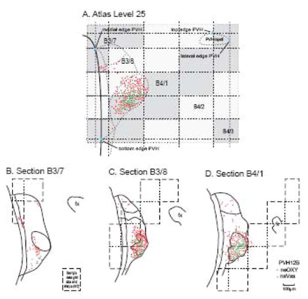
Fig. 6.

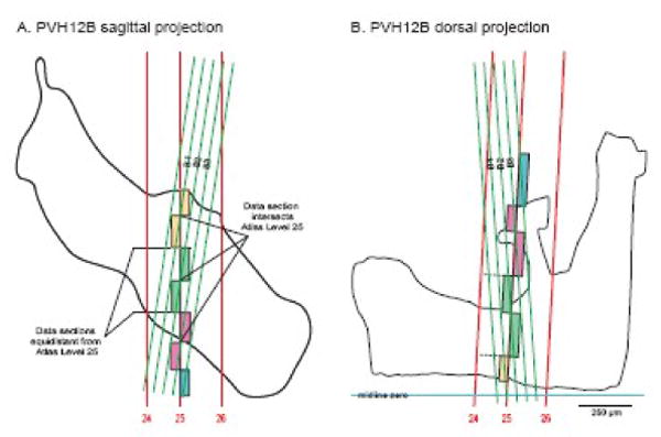
Segmenting regions of experimental sections for data transfer to a reference Atlas Level. For illustration brain PVH12 was used because its plane of section is clearly different than that of the reference Atlas (see Fig. 4). In both the sagittal and dorsal projections, three Atlas Levels (24-26) are shown, along with the relative position of a 1-in-4 series of 15 μm-thick histological sections (series B), three of which contain data that should be transferred to Atlas Level 25, based on principles illustrated in Figure 3. Transition from one experimental section to another (e.g., from B1 to B2) on the target Atlas Level (25) is determined by the point where the line representing each experimental section is equidistant from the Atlas Level. Experimental sections are coded by individually colored boxes that span the area to be mapped onto the atlas template (see Fig. 7). Note that in this example experimental sections are separated by a gap of 45 μm (because every fourth 15 μm-thick section was stained with a particular pair of primary antisera). Sections B1-3 correspond to series B in 4/2-4/4 in Figure 2.

The combined retrograde tracer-immunohistochemical method applied here has been described in detail elsewhere (Sawchenko and Swanson, 1981). In the present study, the serial 15 μm-thick frozen sections cut transversely through the PVH were divided into 4 1-in-4 series (A-D): section 1A was serial to section 1B, which was serial to section 1C, which was serial to section 1D, which was then in turn serial to section 2A, and so on. Thus, in a given series (A, B, C, or D) two sequentially numbered sections (e.g., B 4/3, B 4/4) are separated by three 15 μm-thick sections (a span of 45 μm is missing between them). Three 1-in-4 series of sections were subjected to immunohistochemical processing, each series with two primary antisera raised in different species. The fourth 1-in-4 series of sections was stained with 0.25% thionin (a Nissl stain) for cytoarchitectonic analysis (Simmons and Swanson, 1993, 2008). The immunohistochemical procedure follows standard practice and has been described in detail elsewhere (see Simerly and Swanson, 1987).

Antibodies used for the three exemplar brains described here were: Vasopressin—monoclonal antibody (clone #3-D-VII-αVAS, supernatant at 1:80) from G. Nilaver, Oregon Health Sciences University; Oxytocin—rabbit αOXY adsorbed against arginine-Vasopressin (1:8000) from K. Dierickx, Rijksuniversiteit, Gent, Belgium; CRH—monoclonal antibody (clone PFU83, at 1:1000) from F.J.H. Tilders, Vrije Universiteit, Amsterdam, The Netherlands, and rabbit αCRH (#C-70 raised against rat CRH, at 1:3000) from W. Vale, Salk Institute; TRH—rabbit αTRH (αppT#R363J raised against pre-pro TRH_160-169, at 1:5000) from M. Wessendorf, University of Minnesota; Somatostatin—monoclonal antibody (#SOM-018-αSS_12-14, ascites fluid at 1:200) from Novo Biolabs, Copenhagen, Denmark; Tyrosine Hydroxylase—monoclonal antibody (#P80101-0-to SDS-denatured ratTH, Lot #08413 at 1:10,000) from Pel-Freez Biologicals, Rogers, AR. Secondary antisera used were affinity purified Rhodamine anti-mouse and FITC anti-mouse antibodies from American Qualex (LaMirada, CA) and Tago™ brand Rhodamine anti-rabbit and FITC anti-rabbit antibodies from BioSource division of Invitrogen Corporation (Carlsbad, CA). All secondary antisera were generated in goat.

For maximum resolution all data were acquired by photographing sections with a 10× objective (0.5 n.a.) using a Leitz Dialux 20™ fluorescence microscope and Wild-Leitz™ MPS-46 Photoautomat™ camera system with 35 mm Kodak Elite™ color transparency film (ASA 400). Each field was photographed without movement while successively exposed to UV, FITC, and Rhodamine filters such that discrete photographs of all fluorescent entities in a field were obtained in exact register on three sequential 35 mm slides. In some sections the PVH was too large to photograph completely in one field; here a montage of slightly overlapping 35 mm fields was made. Structural data (ventricles, large blood vessels, overall neuroendocrine parts of the PVH labeled with Fast Blue, individual labeled neurons with a visible nucleus) in the photographs were next transferred manually to 11×14″ projection drawings, which were then scanned and used as templates in Adobe Illustrator™, where perfectly registered data layers were constructed for each PVH neuron type in each photograph, based on combined retrograde labeling and immunohistochemical staining (specifically, retrogradely labeled and nonretrogradely labeled neurons stained with each antiserum). Obviously, digital cameras may now be used for the same purpose, combined with applications like Adobe Photoshop™.

The accuracy of these maps was then checked by direct observation of the original slides under the microscope by two highly trained human experts. In the original maps, labeled cell body outlines were drawn; they were later replaced with symbols about the size of mean neuron diameter. Ultimately, data extracted from each photograph was segregated into 7 layers, with orienting structural outlines in the bottom layer, followed by two neuroendocrine neuron types (retrogradely and immunohistochemically labeled), two non-neuroendocrine neuron types (immunohistochemically labeled only), and two doubly-labeled neuron types (double immunolabeling, with or without retrograde labeling).

3. Major sources of error: types and strategies to reduce them

In this Section, major sources of error are examined sequentially, each one in terms of general principles followed by how it has been dealt with in a specific example. The test bed for this approach was a high-resolution analysis of the spatial distribution and relationship between the various types of neuroendocrine motoneurons in the adult rat PVH —a rich and relatively complex problem (see Swanson, 1991, 1992b). A serial section 3D miniatlas of PVH subdivisions, within the context of a traditional rat brain atlas, has already been published (Simmons and Swanson, 2008), and the global mapping results will be published elsewhere. The goal has been to compare as directly as possible with technology available at the time the precise distribution of two magnocellular neuroendocrine neuron types (OXY and VAS) and five parvicellular neuroendocrine neurons types (CRH, TRH, SS, DA, and GRH)—in 15 μm-thick sections spaced 45 μm apart—and to summarize the results in terms of a single reference atlas. Because all 7 neuron types were not identified immunohistochemically in each section (each contained retrograde labeling to identify positively neuroendocrine neurons, and a combination of two primary antisera to different neuron types), because all combinations of two neuron types were not obtained in a single animal, and because it was important to confirm the reliability of staining patterns, multiple animals had to be used. Attempts to compare as accurately as possible combined retrograde labeling-immunohistochemical staining patterns between the PVH in different animals, and in the right and left PVH of the same animal, led to the strategy reported here.

For description (Fig. 1) it is convenient to divide sources of error associated with the preparation and analysis of histological material from multiple brains into 5 broad categories (intrinsic variability, linear distortions, nonlinear distortions, plane of section differences, and sampling errors) each divided into three sequential phases (premortem, postmortem, histological). The resulting categories are not mutually exclusive or unrelated, and are used simply to facilitate treatment of the many steps that make neurohistology such a complex technical undertaking, and neurohistological results so difficult to analyze in a rigorously quantitative way.

Fig. 1.

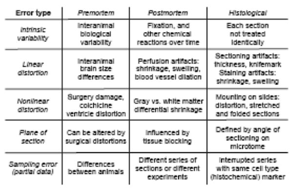
Major sources of error encountered in comparing histological data between brains. They are arranged for convenience and are not mutually exclusive or independent. See text for details.

Strictly speaking, there are three levels of analysis for the problem of comparing data in histological sections. The simplest level deals with differences that occur between adjacent sections from a single brain; the second level concerns comparing data from a group of similar animals whose brains are treated in the same way; and the third level deals with comparing brains from dissimilar animals or from similar animals whose brains are treated in different ways, for example, fixed in different ways or subjected to different histological procedures. A common example would involve comparisons between different transgenic mouse lines, using immunohistochemistry and in situ hybridization. Another example would be the difference between adult male rats used in popular rat brain atlases: Paxinos and Watson (2006) used Wistar rats (290 gram for transverse and horizontal planes, 270 grams for sagittal plane), whereas Swanson (2004) used a single 315-gram Sprague-Dawley animal cut in the transverse plane. In addition, histological procedures used to prepare brains for the two atlases were very different.

3.1. Intrinsic variability

3.1.1. General principles (Fig. 1)

Premortem, the concern here is the basic fact that each animal in a population from a species or strain is different or unique due to a combination of genetic and environmental factors. The range of variability for a particular morphological feature, including those in the brain, is an empirical question that is often very difficult to establish with certainty in mammals, for many of the reasons to be discussed, as is the absolute configuration of a feature in a particular animal (see, for example, Williams et al., 2001). Postmortem there is a range of variables associated with fixation (whether perfusion, immersion, or sometimes none at all) and preparation for histology that must be controlled, including concentration, temperature, and time—because each of them can shrink or expand neural tissue in linear and/or nonlinear ways (see Sections 3.2 and 3.3). During histological processing the key concept is that each tissue section is treated differently unless the process is entirely automated (sometime in the future).

3.1.2. Specific application: minimizing intrinsic variability

This set of problems need not be dealt with in detail here because standard laboratory procedures were followed. Animals of the same strain, sex, and age were used; and housing/physiological status, anesthesia, retrograde tracer injection and survival time, perfusion fixation methods, brain removal, postfixation brain treatment before freezing, brain freezing for cutting, and brain cutting and section mounting procedures were standardized for all experimental animals and carried out by very experienced personnel (Sawchenko and Swanson, 1981; Simmons, 2006). The three exemplar experimental animals discussed below had body weights of 313, 325, and 340 g, whereas the atlas animal's body weight was 315 g. According to data published by Paxinos et al. (1985), their atlas can be used successfully for male or female rats with rats weighing between 250-350 g.

3.2. Linear distortion

3.2.1. General principles (Fig. 1)

Because neural tissue is a complex mixture of gray and white matter, which have different densities, physical strengths, and chemical compositions, it is unlikely that whole brains, or even smaller pieces, ever undergo strictly linear scaling due to changes in life cycle, physiological manipulation, disease, or histological processing. Nevertheless, error may often be reduced considerably by applying linear spatial corrections for the three cardinal axes. This can be accomplished easily for digital brain photographs or vector graphics brain maps with applications like Adobe Photoshop™ or Adobe Illustrator™ in the x and y (and z for a stack of maps) axes, with different or equal values for each.

Premortem the major sources of roughly linear differences relate to animal age and sex. Postmortem factors relate most obviously to differences in fixation parameters before tissue cutting. Perfusion pressure differences between animals result in different amounts of tissue swelling from hydrostatic pressure, which is often most apparent in blood vessel diameter. Different fixatives or different fixative concentrations, combined with different fixative solution molarities, also lead to different amounts of tissue shrinkage or expansion due to osmosis combined with differential amounts of tissue fixation. Histological factors may be divided into two broad classes: sectioning artifacts and staining artifacts. The former includes tissue compression perpendicular to the knife-edge; variations in section thickness, particularly when the brain is cut manually, and knife marks perpendicular to the knife edge due to debris on the knife. The latter include tissue shrinkage or swelling due to cumulative osmotic effects of the various solutions used in staining and physical distortions introduced during mounting procedures.

3.2.2. Specific application: correcting linear distortion

As far as possible, all experimental animals were housed and treated the same, and histological procedures were also standardized. The major problem here was comparing PVH data from sections of experimental animals with the corresponding reference atlas Atlas Levels: the former brains were cut frozen without embedment, whereas the latter were derived from a celloidin-embedded brain that underwent considerable shrinkage during processing. This is a classic example of comparing histological data from similar brains treated with different histological methods. For example, in determining stereotaxic coordinates for the reference atlas it was found that linear corrections of 139% in the mediolateral axis, 161% in the dorsoventral axis, and 127% in the rostrocaudal axis would produce the approximate dimensions found in a frozen-sectioned brain (Swanson, 1992).

The reverse situation applies here: the goal is to map experimental data from a well-defined nucleus onto a reference atlas. For this a simple, graphic, geometric solution relying on clear fiducial marks in the brain was developed (Fig. 2) and implemented in Adobe Illustrator™. After determining the angles between experimental brain and atlas brain planes of section (Section 3.4.2), a geometrically accurate model of a long series of serial histological sections is prepared (and in this case set to 15 μm thickness each, corresponding to section thickness in experimental brains at the time of cutting). Then, the number of serial experimental sections between two rostrocaudally placed fiducial marks (c and h in Fig. 2) is determined for each brain. Finally, a linear correction factor is applied to the horizontal axis of the experimental section model such that lines representing sections containing the two fiducial marks in the experimental brain and center points of symbols for fiducial structures in the reference atlas brain overlap perfectly. This provides a simple linear scaling of the experimental brain rostrocaudal axis relative to the reference atlas. Subsequent alignment of sections, linear scaling in the dorsoventral and mediolateral axes, and nonlinear warping are discussed in Sections 3.5 and 3.3, respectively (also see Fig. 12B, C).

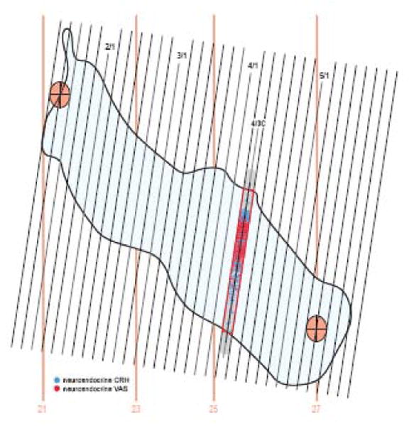
Fig. 2.

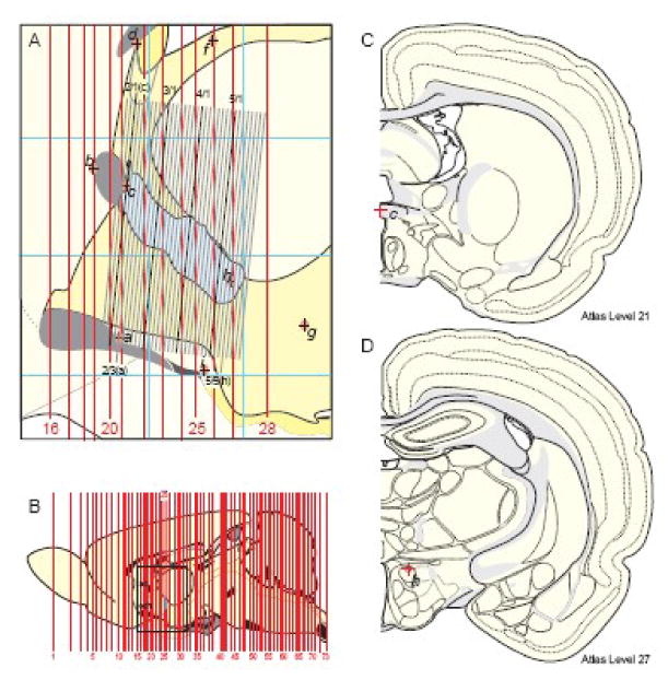
Graphical comparison of brain section levels represented in a reference atlas with a serial set of tissue sections from an experimental brain. A. This is a midsagittal view of the rat forebrain region surrounding the PVH (blue outline of its border), indicated by the rectangle in (B), which is a midsagittal view of the rat brain along with a thick red line indicating the position of Atlas Level 25. In A, Atlas levels 16-28 are indicated with vertical red lines (whose thickness is to scale, for these 40 μm-thick celloidin sections), whereas a 1-in-4 series of 15 μm-thick frozen transverse sections from another (experimental) brain cut at a different plane of section is shown to scale as the tilted array of black/gray lines. Each black/gray line indicates a section and space between black/gray lines indicates the presence of three sections belonging to the other three1-in-4 series; that is, each line and space indicates a block of 4 serial 15 μm-thick frozen sections (60 μm total). Every 6th line is black indicating that blocks of 6 successive 1-in-4 sections (one black and 5 gray) were mounted on each 1×3 inch microscope slide (notation at top: series of 6 1-in-4 series/number of series). Light red ovals with internal cross indicate the position of fiducial marks: a, rostral end of the suprachiasmatic nucleus; b, rostral edge of the anterior commissure; c, caudal edge of the suprachiasmatic nucleus; d, rostral edge of the subfornical organ; f, rostral tip of the medial habenula; g, posterior part of the dorsomedial nucleus of the hypothalamus; h, dorsal part of the anterior hypothalamic nucleus; i, rostral end of the arcuate nucleus. The orientation of the experimental series relative to the atlas orientation was determined geometrically. The sections with two more or less vertical fiducials (a and c; 2/3 and 2/1, respectively) was determined and then lined up on the atlas projection simply by rotating and aligning the block of experimental sections. Then the number of experimental sections between atlas fiducials a and h was determined, and a linear correction factor was calculated to fit the experimental series between atlas fiducials a and h. Thin blue horizontal and vertical lines indicate stereotaxic coordinates 1 mm apart. B. This is a sagittal outline of the reference Atlas brain that was scaled to the dimensions of the frozen sections for convenience of computer graphics manipulations as described in the text. Abbreviations: ac, anterior commissure; och, optic chiasm. C and D. Drawings of transverse Atlas Levels 21 and 27, whose rostrocaudal position is shown in parts A and B. They are shown to illustrate the position of fiducial marks c and h (labeling the red crosses in C and D, respectively) from part A. All parts adapted from Swanson (1998).

Fig. 12.

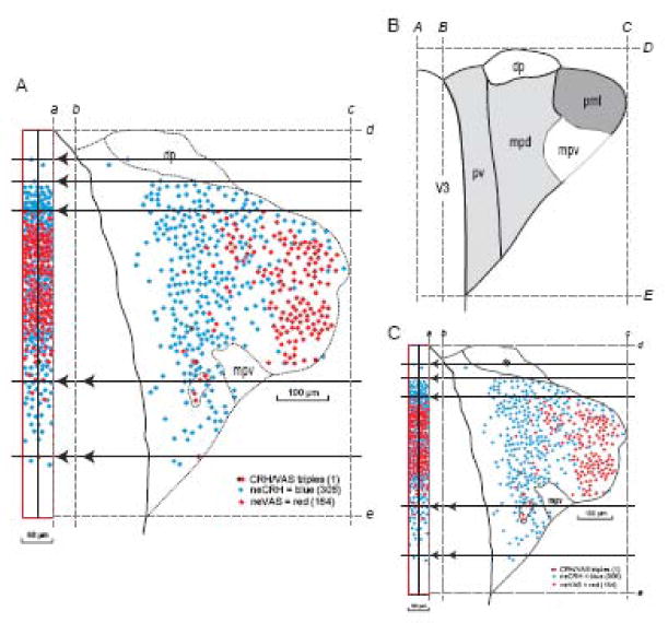
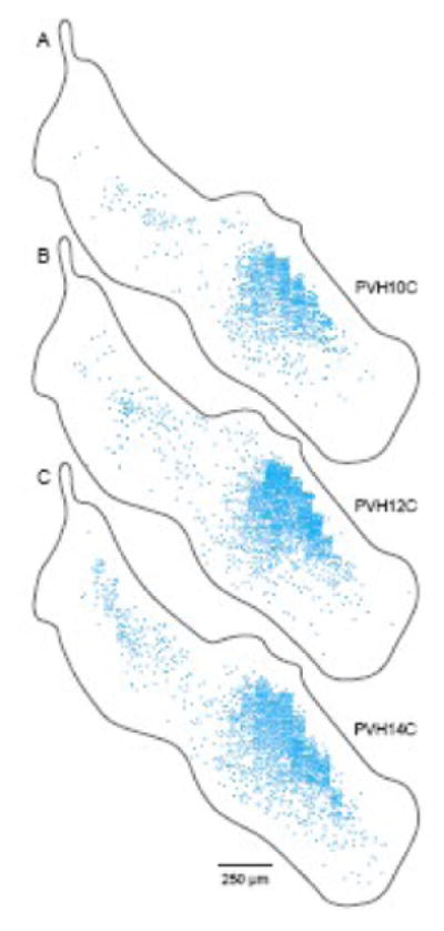
Compression of PVH data mapped in the transverse plane into a slice of a sagittal projection map for spatial distribution overview (A) and linear scaling of the data to a reference Atlas Level (B, C). A. Data from a 15 μm-thick transverse section of the PVH is moved horizontally (dashed lines with arrowheads) into a vertical bin on the left, scaled to be 60 μm wide in a sagittal projection map of the PVH (Fig. 2), using principles illustrated in Figure 11 and implemented manually here. Mapped in this histological section were retrogradely labeled neurons that immunostained for CRH (neuroendocrine CRH neurons, neCRH; blue), retrogradely labeled neurons that immunostained for VAS (neuroendocrine VAS neurons, neVAS; red), and one neuron that appeared to be triply labeled (numbers in parentheses are total number of indicated neuron types with a visible nucleus in the section). Margin of the third ventricle is black and dotted lines indicate subdivisions of the PVH determined from nearby Nissl-stained sections. From brain PVH12C, 4/3 (CRH & VAS double immunostaining with fast blue retrograde labeling). Dorsal (top), ventral (bottom), medial (left), and lateral (right) bounding lines were interpolated between Nissl-stained sections 12A 4/3 and 12A 4/4 position lines on the sagittal projection. Also see Fig. 10A for CRH immunostaining plotted a different way for this section. B, C. Parts A and B are to scale, so a first step in fitting the data from a histological section (A) to a corresponding reference Atlas Level (B) is to perform linear scaling in the horizontal and vertical axes. The approach to accomplish this here for the PVH was to establish in each section its medial border (b, B), lateral border (c, C), dorsal border (d, D), and ventral border (e, E), all in relation to the vertical midline of the brain (a, A). The scaled histological section (C) is then produced with the Scale Tool of a graphics program, using horizontal and vertical percentages calculated from the ratios BC/bc and DE/de, respectively. The next step would involve the grid transfer method described in Figures 6-8, unless the reference atlas and experimental brain were cut in the identical plane of section, in which unlikely case nonlinear warping of C onto B could be performed.

3.3 Nonlinear distortion (Fig. 1)

As already suggested, nonlinear distortions can and usually do creep into virtually every step along the way toward the extraction of data from histological sections of the brain, resulting in a different pattern in every section. For example, premortem distortions can be induced by surgical procedures like the insertion of injection pipettes or cannulae or the creation of lesions, or by intraventricular injections, which usually cause noticeable expansion of the ventricular walls, in a pattern depending on where the injection is made (for example, the lateral or fourth ventricle). Postmortem changes are most obvious because of differential distortion of gray and white matter (Section 3.2.1). But perhaps the most severe and unpredictable nonlinear distortions arise when mounting individual tissue sections on glass (see Swanson, 2001). Great skill on the histologist's part can certainly reduce these distortions, but cannot eliminate them. The sections are relatively very thin (say 15 μm thick by 10,000 μm high by 15,000 μm wide for a typical rat brain section) and the tissue relatively weak, no matter how well fixed. A good analogy would be trying to lay a large, thin crepe down flat on a plate over and over again in exactly the same way, but by comparison this would be an easy task.

The result is that each tissue section has a distinct, pervasive pattern of nonlinear distortions, often accompanied by tears, bubbles, and folds, which by comparison are almost impossible to correct adequately. This is not the place to review the many methods for warping the shape of one brain section/slice to another; for a good introduction see Toga (1999). However, it is worth recalling that these methods rely on mathematically transforming a set of fiducial points and/or lines in one slice to a corresponding set in another slice. Thus, warping accuracy is proportional to the number of fiducial marks and in transferring data from an experimental section to a reference atlas level, accuracy will be greatest if all structural information in the reference atlas level is identified and marked in the experimental section.

It is probably also worth noting that all warping of brain slices is relative because there is no way to know the absolute in situ histological structure of a brain. This is because there are no inflexible internal fiducial structures in this entirely soft tissue (see Toga and Banerjee, 1993; Streicher et al., 1997; Weninger et al., 1998). Unlike the body, the brain does not have a hard internal skeletal system to provide significant impediment to deformation, although the surrounding skull does define a physical constraint for the size and shape of the adult brain surface.

3.4. Plane of section artifacts

3.4.1. General principles (Fig. 1)

It is generally true that every brain is sectioned in a different plane (unless convincingly demonstrated otherwise in fortuitous exceptions). For the sake of discussion comparisons between sections from an experimental brain and a reference brain will be made. Premortem, deviations in an experimental brain relative to a reference brain can be induced by surgical manipulations already mentioned (introduction of pipettes and cannulae, intracerebroventricular injections, lesions). The spatial extent of these typically nonlinear distortions may be more or less localized depending on severity. Postmortem the major factor is how the brain is blocked to mount on the microtome stage for sectioning, assuming the entire brain is not sectioned without blocking. A number of devices for holding the brain and blocking it in a standard plane have been described, and they certainly reduce variability relative to freehand blocking. For histological processing, the obvious variable is the actual angle of sectioning, determined by how the brain block (or whole brain) is oriented in three dimensions on the microtome stage. When all is said and done, the actual sectioning angle of each brain, relative to a reference brain, needs to be measured.

When comparing a histological staining pattern in a brain section from an experimental animal to the parceling in a reference atlas, it is a common experience that part of the staining pattern (say in the top of the section) is on one Atlas Level, and the rest of the staining pattern (say in the bottom of the section) is on an adjacent Atlas Level. A formal analysis of the problem is illustrated in Figure 3, where for simplicity it has been reduced from three dimensions to one. Note that when there is a plane of section difference, there can be only one point or location where the experimental section (E_n) and a given Atlas Level (R2, in Fig. 3A) are identical. Moving away from this point, discrepancies between experimental section and Atlas Level steadily increase, and the magnitude of these discrepancies obviously is also greater the greater the angle between sections (no error when the angles are equal). As a result, grave errors result when systematically transferring data from experimental section to Atlas Level; for example, histological staining that is actually in structures b and y are transferred inappropriately to structures m and c, respectively.

Fig. 3.

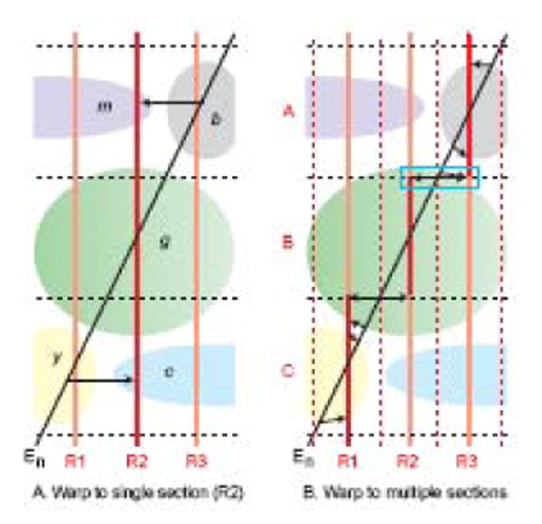
Plane of section effects on data transfer from histological section of experimental brain (E_n, black) to reference Atlas Levels (R1-R3, red and light red). Morphological features (b, c, g, m, y) of the brain are assumed to be the same in the experimental and atlas brains, and for simplicity the problem is reduced from three dimensions to one. A. If experimental data (E_n, black) is warped or transferred (thin black arrows) to a single Atlas Level (R2, red), misidentifications occur (structure b as m, and y as c), and their magnitude increases with greater angle between the two sections, with greater distance from the point of intersection in structure g, and with smaller and/or more convoluted morphological features. B. Transfer error is reduced significantly if data from the experimental section is mapped onto segments (A-C, red) of three adjacent Atlas Levels (R1-R3) instead of one (R2, Fig. 3A), although distortions remain (indicated by the horizontal black arrows, especially obvious in the blue rectangle. Adapted with permission of the Publisher (Elsevier) from Swanson (2004).

In this example, experimental data representation is obviously more accurate if it is represented on three Atlas Levels (R1-3, Fig. 3B) instead of one (R2) because here there are three intersection points, and data transfer occurs over shorter distances (A-C, black) from intersection points. From the geometry it is obvious that transfer error is reduced with smaller plane of section angle difference; transfer between larger, more homogenous, and less convoluted morphological features like cell groups or fiber tracts; and more closely spaced Atlas Levels.

3.4.2. Specific application: determining plane of section

This Section deals with a method for determining plane of section angle, and an approach to minimize plane of section artifacts in transferring data from experimental sections to a reference atlas. The method we developed for determining plane of section relies on the identification of clear, readily identifiable fiducial points in the brain as seen in Nissl-stained sections (Swanson, 1992, 1998). For example, comparing the right and left rostral tips of a number of structures along the rostrocaudal axis, it was determined that our atlas brain was cut 4° off perpendicular to the midline (from true transverse), with the right side caudal to the left (Fig. 4, dorsal view). This was calculated by simple triangulation, knowing the distance between fiducial points, and the number of histological sections (of known thickness) between the right and left fiducial point.

Fig. 4.

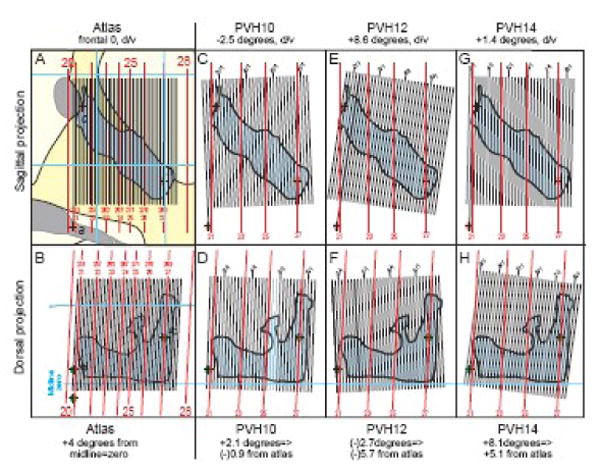
Empirically determined plane of section in three experimental brains compared to the plane of section in a reference Atlas (Swanson, 2004). Although these experimental brains were prepared carefully in a brain blocker (Swanson, 2004), the actual plane of section was clearly different in each one, as determined by the method illustrated in Figure 2, and described in the text. The case where the atlas plane of section equals a (hypothetical) experimental brain plane of section is shown in A and B, where the atlas midsagittal projection was scaled to match the dimensions of the experimental brain (as in Fig. 2B). For each brain the plane of section is shown as viewed from the side (sagittal view: A, C, E, G) and from the top (dorsal view: B, D, F, H).

To calculate plane of section for an experimental brain it is convenient first to make the brain's midline vertical to account easily for one degree of freedom. Due to nonlinear distortions the midline is never perfectly straight in a histological section, but it can be approximated relatively easily using multiple internal landmarks. To determine right-left deviations (from true transverse, that is, perpendicular to the longitudinal axis), and deviations from vertical (dorsoventral axis relative to the dorsoventral axis of the reference Atlas Levels) it is important to choose fiducial points as far apart as possible, but in the case of mapping restricted areas (like the PVH here) as close as possible to the boundaries of the restricted area. For determining the right-left difference from true transverse in three experimental brains used for PVH mapping, the dorsal part of the anterior hypothalamic nucleus (h in Figs. 2 and 4) on the right and left side was chosen. Based on this fiducial it was determined that the angles were +3.1°, -1.7°, and +9.1° from true transverse (Fig. 4, dorsal view), despite careful use of a brain blocker (Swanson, 1998, Fig. 6 there). For determining deviation from Atlas vertical, two relatively nearby midline fiducials, the rostral end of the suprachiasmatic nucleus and the caudal end of the anterior commissure (a and c, respectively, in Figs. 2 and 4), were chosen. Based on these fiducials the three experimental brains were cut -2.5°, +8.6° and +1.4° from Atlas vertical (Fig. 4, midsagittal view).

3.5. Section alignment and staining pattern alignment

Because there is no rigid scaffolding within the brain, it is not possible to reconstruct the absolute physical alignment of histological sections (Section 3.3), although a number of methods reduce error considerably. One seldom used possibility involves making small diameter holes (say with a strong pin) through the longitudinal length of the brain on the right and left side and then using the two holes in each section as alignment guides. The most recent possibility involves using an MRI image of the in situ brain as a guide for aligning subsequent histological processing of the same brain (see MacKenzie-Graham et al., 2004). The method used to align our reference atlas in 1992 was simple in principle. First, vector drawings of all Atlas Level sections were aligned vertically along the midline, which provides a zero point for the midline of sections from the bilateral brain, and then arranged sequentially from rostral to caudal with proper spacing based on section thickness and number of unused sections between Atlas Levels. Then the dorsoventral height of each section drawing was determined relative to the others by fitting it to an outline of a brain photographed from the side (see Fig. 2A).

Aligning drawings of frozen sections from the three experimental brains with staining in the PVH was accomplished in a similar way, this time using outlines of the PVH as viewed from the side (a midsagittal projection or view) or from the top (a dorsal projection or view) in the Atlas brain as a reference (Fig. 4). The method for constructing these two projection outlines from the 37 serial sections of the Atlas brain containing the PVH has been described elsewhere (Simmons and Swanson, 2008). Very simply, sequential drawings of the PVH outlines and staining patterns within it (for an experimental brain) were placed in sequence in the Layers panel of Adobe Illustrator™ (aligned along the brain midline), and then each drawing was moved up and down to fit within the properly scaled outline of the PVH (Figs. 5 and 6). As mentioned in Section 3.2.2, once this stage of alignment has been reached, linear scaling in the x and y axes may be applied to the drawings to achieve a better fit within the outlines, and once all this aligning and linear scaling has been done, nonlinear warping may be carried out to create smooth continuity between drawings (or photos) of experimental sections, as well as between experimental brain section drawings and Atlas Level drawings.

Fig. 5.

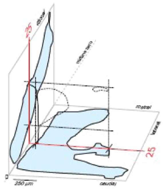
A framework for aligning histological sections to a reference atlas. This 3D drawing shows sagittal (left, blue) and dorsal (bottom, blue) projections of the PVH for the reference atlas (see Figs. 2 and 4), along with Atlas Level 25 (red lines with PVH outlined with dashed lines and margin of third ventricle indicated in black; see Figs. 2, 4, and 7). Experimental series of sections can be aligned to these outlines, sequentially, in the Layers panel of a computer graphics application (Fig. 6), after plane of section has been determined (Figs. 2 and 4).

Aligning sections from a brain is one thing, but aligning different staining patterns, say for two different antigens or mRNAs, between different sections of a brain, or between different brains, is quite another. As a general rule, the best way to compare two or more histological staining patterns is the direct approach of multiple staining (with clearly distinguishable colors or reaction products) on the same tissue section (and even better in serial sections) so the patterns can be observed together (see Micheva and Smith, 2007). As the number of staining patterns increases, and underlying methods multiply, this is not always possible. Fortunately, there is a simple solution for comparing different histological staining patterns in different sections at comparable levels of the brain: if pattern x in one section is to be compared to pattern z in another section, then pattern y that is found in both sections should also be displayed with double-labeling methods as a fiducial marker in both sections. If pattern y in the two sections can be made to overlap with proper section alignment, linear warping, and nonlinear warping, then a very good rendering of the relationship between x and z can be inferred.

3.6. Data transfer from experimental sections to Atlas Levels: grid transfer correction method for plane of section artifacts

Based on our experience with the spatial mapping of neuron type distribution in the PVH, a visual geometric method was established for decreasing plane of section artifacts when transferring data to Atlas Levels of a reference atlas from aligned and distortion-corrected series of section drawings from experimental animals, so that patterns from different series and different animals could be overlain, aligned, and compared more accurately in the Layers panel of Adobe Illustrator™. The procedure is based on principles illustrated in Figure 3, but applied to specific instances in both the midsagittal and dorsal projections in a geometrically accurate way (Fig. 6, also see Fig. 4). In essence it identifies “parallelograms” in experimental sections that map most closely onto a particular Atlas Level (Fig. 7). Data within the experimental section gridwork is transferred or moved systematically to the Atlas level, all of this being accomplished in the Layers panel of Adobe Illustrator™ (Fig. 8).

Fig. 7.

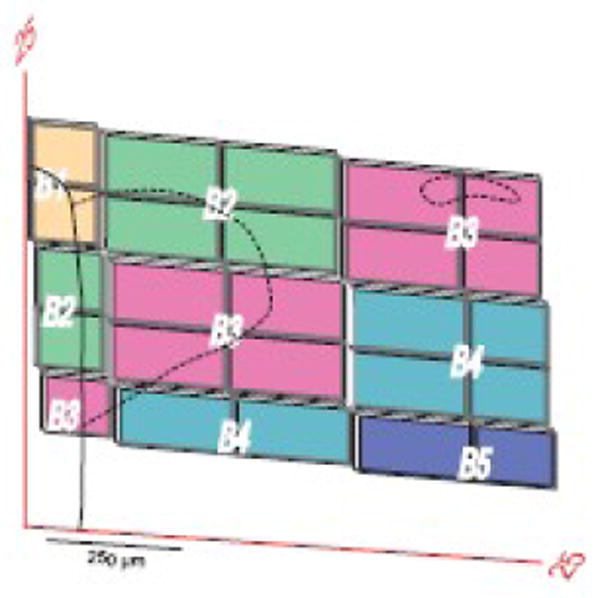
Example of parts of experimental sections used to transfer data to a reference Atlas Level. The derivation of this trapezoidal grid is illustrated in Figure 6 with plane of section data from Figure 4. Note that at this transverse level of the PVH (Atlas Level 25), data from 4 experimental sections (15 μm-thick, spaced 45 μm apart; B1-B4) is transferred systematically to Atlas Level 25. The number of elements in the grid is proportional to the difference in plane of section (Fig. 3) and would equal one for an experimental section cut in exactly the same plane as the reference atlas and exactly overlying the Atlas Level. The PVH is outlined with dashed lines; the small part in the upper right that is detached from the main body of the nucleus at this level is the lateral tail of the dorsal zone of the medial parvicellular part (Simmons and Swanson, 2008). The heavy black line to the left indicates the wall of the third ventricle.

Fig. 8.

Data grids from a series of histological sections mapped onto a reference atlas level. In this case, neuroendocrine neurons immunostained for oxytocin (neOXY, red) or vasopressin (neVAS, green) from three adjacent sections (B-D) 1-in-4 series B of animal PVH12B are mapped on Atlas Level 25 (A), based on principles illustrated in Figures 2-7 and 12. Borders of the PVH and its parts were obtained from the adjacent Nissl-stained series A. Data grids for the Atlas Level and histological sections are not identical in size because the former (A) is from a celloidin-embedded brain whereas the latter (B-D) are from a frozen-sectioned brain. Abbreviation: PVHmpdl, paraventricular hypothalamic nucleus, medial parvicellular part, ventral zone, lateral wing.

Unless serial sections are used, there is usually between “parallelograms” a discontinuity or space that is proportional to the distance (number of sections) between mapped sections (Fig. 7). In practice this discontinuity is usually barely noticeable, but occasionally an obvious, irregular gap of apparently missing data was observed in the space between two “parallelograms” of the grid. Careful inspection revealed that these more obvious gaps occur where curvature of the bounding surface (the PVH in this instance) is greatest (Fig. 9). This pointed to the geometric fact that in nonserial series of sections, the space between “parallelograms” of the transfer grid is curved as a function of boundary curvature, so that, strictly speaking, all of the “parallelograms” may not be parallelograms—if the curve on either side of the gap is slightly different. Furthermore, at the extreme where there is no curvature between the boundaries of a structure in experimental and reference brains, and there in no difference in plane of section, there would be no gap between parallelograms of the grid. Thus, the grid transfer method produces a checkerboard effect that becomes greater with increasing density of data points, curvature of bounding surfaces, plane of section difference, and gap between mapped sections.

Fig. 9.

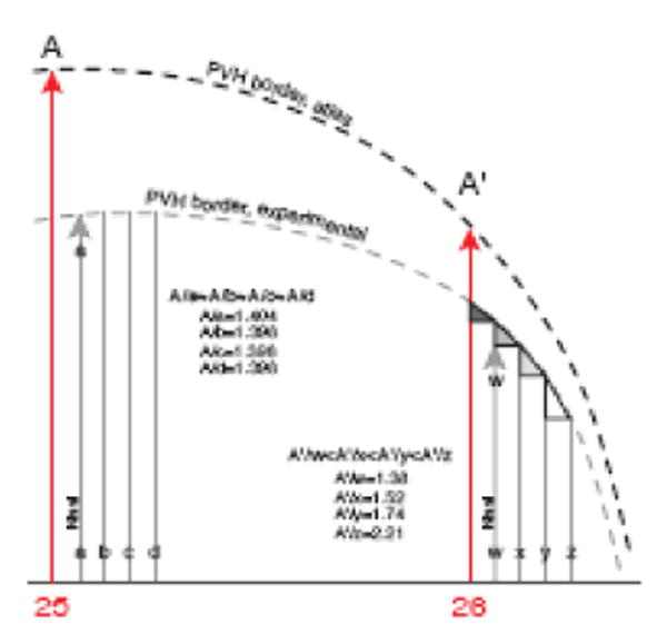
Problems exaggerated near highly curved surfaces. Distortion and apparent error may be introduced when moving experimental data onto a reference Atlas Level in regions where the border of a structure (e.g., nucleus or fiber tract) curves sharply. For illustration of underlying geometric principles lines representing Atlas Levels 25 and 26 (red) are displayed in a sagittal projection including the PVH (dashed line). Lines a-d and w-z represent two sets of four serial sections from an experimental brain with data that map onto the atlas templates, in the same plane of section as the Atlas Levels in this simple example. PVH boundaries for the experimental and reference brains are roughly parallel and proportional, but not overlapping. Thus, experimental data are scaled (nonlinearly in this case) to fit the atlas template. Distance to the edge of the PVH can change rapidly—even within the thickness of a single section, as indicated by different-sized triangles at the top of section lines w-z. Therefore, data from adjacent sections might appear to have a gap, notch, or step in distribution at the edge of a highly curved surface, a “checkerboard” artifact (see Fig. 14) that is more extreme if the curve is in three dimensions. When mapped data are taken from 1-in-4 series of sections, as in Figure 7, such an apparent distortion is amplified, and data grids must be individually scaled, either mathematically or manually (which is often easier and relatively useful). Note that the first section in each block is Nissl-stained for cytoarchitecture.

A comparison of two methods for combining data from different animals (each sectioned in a slightly different plane) in a composite map of PVH neuron types is presented in Figure 10. The simplest, traditional approach illustrated on the left involves aligning as well as possible the maps and then simply collapsing the data onto a single plane, a procedure that is now done most easily in the Layers panel of a graphics application like Adobe Illustrator™. The grid transfer correction method was used to create the summary map on the right, which is considerably more faithful to the appearance of individual neuron types when observed in a histological section cut at this angle at this rostrocaudal level.

Fig. 10.

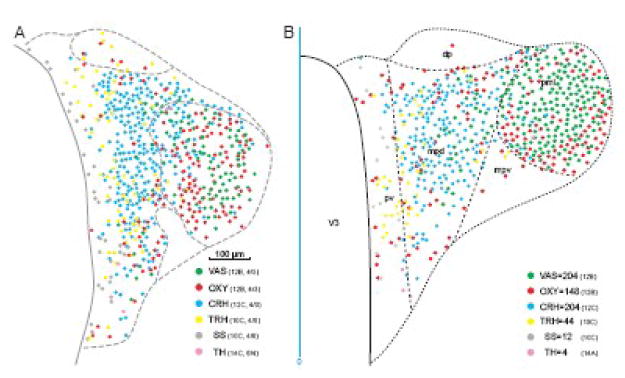
Effect of correcting for plane of section artifacts. A. This is a composite map of 4 immunohistochemical sections from three different animals, chosen to be as close as possible to the same rostrocaudal level of the PVH, corresponding to Atlas Level 26. One section (PVH12B, 4/3) was doubly labeled with antisera to vasopressin (VAS) and oxytocin (OXY), another from the same animal (adjacent section C, 4/3) with an antiserum to corticotropin-releasing hormone (CRH), another from a second animal (PVH10, section C, 4/8) with antisera to thyrotropin-releasing hormone (TRH) and somatostatin (SS), and yet another from a third animal (PVH14, section C, 6/4) with an antiserum to tyrosine hydroxylase (TH, a marker for dopamine). They were aligned manually using available landmarks including the third ventricle (V3), base of the brain, and outline of the PVH (see Figs. 5 and 6). B. Summary map of neuroendocrine neuron type distribution on Atlas Level 26, with each peptide mapped separately from multiple sections using the grid transfer method for correcting plane of section artifacts (Fig. 7). In particular, the distribution of VAS and OXY in the lateral zone of the posterior magnocellular division (mpl) is depicted much more accurately, as judged by photographs of double immuno-stained sections at just this level and orientation, than in the direct composite approach of part A. The vertical blue line indicates midline (midline zero); other abbreviations for PVH parts: dp, dorsal parvicellular; mpd, medial parvicellular part, dorsal zone; mpv, medial parvicellular part, ventral zone; pv, periventricular.

3.7. Sampling errors and volumetric data

3.7.1. General principles (Fig. 1)

There is no need here to review comprehensively this vast, complex topic. Instead, we will summarize the most relevant problem to the topic at hand—dealing with partial data sets, and thus of necessity data sampling, because serial sections are not used and because data is derived from multiple animals. Premortem, intrinsic differences between animals, and surgical interventions, can lead to sampling problems, whereas postmortem factors include using different series of sections from the same animal or from different animals or experimental conditions. During histological processing the major factor is the fact that nonserial, interrupted series of sections, from the same and/or different brains, are used. However, section thickness variability in a particular brain and many other factors can influence sampling accuracy, and thus variability.

3.7.2. Specific application: reconstructing and resampling three-dimensional data

The goal of the approach described thus far is to summarize data from interrupted series of sections from an experimental brain cut in one plane of section on the nonserial Atlas Levels represented in a reference brain assumed to be cut in a different plane of section. The result of this procedure is that histological data patterns from any and all experimental brains can be viewed in register over individual reference Atlas Levels. Interesting new approaches will emerge when high-resolution, 3D computer graphics models of the brain that can be resliced in any plane are available for data population. In principle, series of histological sections could be “fitted” to the surface outlines of the model by linear and nonlinear warping, and then data extracted onto atlas drawings sliced in the same plane and location as the histological sections. However, when the brain model would then be viewed, the data would appear as a series of sheets separated by gaps; for example, in data from a 1-in-4 series of 15 μm-thick sections, there would be 15 μm-thick sheets with data, separated by a gap of 45 μm with no data (Fig. 11).

Fig. 11.

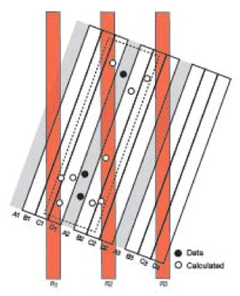
Filling data gaps in 3D space and data resampling model. The block of slices (A1-D4) represents 12 serial histological sections divided into three consecutive 1-in-4 series, with series A stained for tissue component x (filled circles). For simplicity, x is sparse, and only three discrete instances were observed, all in section A2 (none in A1 and A3). To generate a more realistic view of what actually occurs in the tissue, a statistical model of the data could be calculated for the adjacent sections that were not stained for x (open circles in the dashed rectangle). If this is done, the data model can be resliced in any direction (calculated slices R1-3) and a statistically meaningful pattern observed. If “empty” space is not populated with estimated data, reslicing as indicated yields a degraded data pattern proportional to the proportion of empty space. The resliced plane of section could be that of a reference atlas (for example, Fig. 2B). For geometrical accuracy and simplicity the model has been constructed at the section thickness set on the microtome, not at the time of section photography.

The most obvious solution would be to fill the empty space with statistically similar, calculated “data”. This would provide a data model that appears smooth when viewed from any angle, and would allow the data model to be sliced at any angle and still appear complete. This functionality would allow data to be entered into the brain model at any plane of section, and then resliced for viewing in the three familiar, cardinal planes of section: transverse, sagittal, and horizontal.

It is critical to point out several complications associated with such procedures. First, tissue sections are cut at a particular thickness on a calibrated microtome. In general, however, by the time sections are photographed their thickness has changed (they have usually collapsed), and is often irregular, being thicker in the region of fiber-rich white matter and thinner in the region of neuropil-rich gray matter. In any quantitative analysis this change in thickness must be taken into account. For the model presented in Figure 11, data has been placed in a rectangular array of “bins” with a bin width equal to the physical thickness set on the microtome. Second, the complication of double-counting errors and truncated structural features when analyzing tissue sections are well known and must be accounted for with appropriate statistical analysis (see Konigsmark, 1970; Schmitz and Hoff, 2005). And third, appropriate statistical methods must be used to “fill in the data gaps.” This requires a statistical validation of sample variance at each physically mapped interval to provide an objective measure of how wide a gap can in fact be permitted within an acceptable range of error. In other words, it is important to “normalize” the sampled data to reconstruct as reasonably as possible the missing or unsampled data in the gaps, with the goal of reconstructing an overall distribution pattern as faithfully as possible. A reasonable approach to this problem has been worked out for quantitative stereology (Schmitz and Hoff, 2005), but doing the same for the type of data presented here is beyond the scope of this review.

4. Two-dimensional projection data maps

When dealing with the 3D spatial distribution of complex neuron populations it is sometimes useful to summarize them as projections on a flat plane, viewed perhaps from the top, side, and front. Creation of PVH projection outlines as viewed from the top (dorsal view) or side (sagittal view) was described elsewhere (Simmons and Swanson, 2008), and they are illustrated here in Figures 2, 4, and 5. A method for using these projection outlines was developed as part of the work reported here, and shares many of the principles described in the preceding section. The strategy is simple. Data from a drawing in one plane (say transverse) is moved systematically (in a computer graphics application like Adobe Illustrator™) to compress it into a slice (Fig. 12) that fits into a corresponding slot in the correctly scaled projection outline, say sagittal (Fig. 13). Then the procedure is repeated with other, sequential transverse drawings until the corresponding projection is filled and the resulting map is complete. A distinct advantage to this procedure is the ability to display cumulatively in a single image data obtained from thirty or more sequential sections in a different orientation. Though medial-to-lateral information is no longer evident in such a sagittal projection, the comprehensive overview of caudal-to-rostral and dorsal-to-ventral data distribution throughout the target area (PVH) is very informative. As described above (Section 3.6) for the grid transfer correction method, projection mapping suffers from a staircase effect that becomes more obvious with increasing data density, curvature of bounding structures, and space between mapped sections. An example of this effect for neuroendocrine CRH neuron population distributions in three different animals is shown in Figure 14.

Fig. 13.

Data for one bin of the PVH sagittal projection summary map. The data for CRH and VAS neuroendocrine neurons on a transverse section is replotted on this schematic sagittal projection of the PVH outline, taking the 60 μm-thick “slice” or bin generated in Figure 12 (gray outlined area at 4/3). The section was from brain PVH12, 1-in-4 series C, slide 4/section3 (for relative location, see Fig. 4E, F). By reiterating this process for each 1-in-4 section of the series, the entire sagittal flatmap is populated, yielding one view of a comparison of distribution patterns for these two cell types. In this way an accurate representation of data distribution in the sagittal plane throughout the rostrocaudal extent of the PVH can be shown, with no information about mediolateral data distribution. The same procedure can be done for the PVH dorsal projection where medial to lateral data distribution is preserved throughout the rostrocaudal extent of the PVH (Figs. 4-6).

Fig. 14.

Distribution of neuroendocrine CRH neurons (blue dots) in three different animals viewed on sagittal PVH projection maps (A-C). Data from one 1-in-4 series of 15 μm-thick frozen sections in each animal were transferred as shown in Figures 12 and 13 onto a sagittal projection map of the rat PVH. The staircase effect in the region of greatest neuron density (centered around the transverse level illustrated in Fig. 10) is due to three factors (see Fig. 9): high neuron density, great curvature of the bounding region (PVHmpd), and use of an interrupted data set (here a 45 μm gap between 15 μm-thick sections). Series PVH10C was stained with the sheep antiCRH antiserum, whereas series PVH12C and PVH14C were stained with the rabbit antiCRH antiserum.

5. Review of the data preparation protocol

It may be helpful here to review in outline the basic steps—after the brain has been cut, and the sections stained and mounted—involved in the graphical alignment of an experimental brain with a reference atlas, and the grid transfer correction method developed to transfer histochemical staining patterns to Atlas Levels.

Phase I: Photograph sections and prepare data maps

Sections are photographed at an appropriate magnification for unambiguous data identification, and then data is transferred to primary drawings. In the current work this phase was accomplished manually from 35 mm color photographs; digital photography is now a practical alternative.

Phase II: Create separate maps, maintained in register, for different data types in the primary drawings

This phase was also done manually for the current work; but is now practical as well with applications like Adobe Photoshop™ and Illustrator™.

Phase III: Convert data layers to computer graphics files

Again, this phase was accomplished manually here, keeping computer graphics files in register in the Layers panel of Adobe Illustrator™.

Phase IV: Photograph and draw accompanying Nissl-stained series

This is easily accomplished for digital photographs in Adobe Photoshop™. It is important to note that Nissl-stained sections are shrunken compared to immuno-stained sections (because of differences in histological processing), so different linear correction factors are applied later when aligning with each other, and with reference Atlas Levels.

Phase V: Align and scale the experimental Nissl-stained series

The basic goal here is to place the series in order in the Layers panel of a computer graphics application, and then to apply an appropriate linear scaling factor to the series, bringing it in register with the immuno-stained series. Blood vessels running through adjacent Nissl- and immuno-stained sections provide excellent fiducials for determining scaling factors.

Phase VI: Determine orientation of experimental Nissl-stained series relative to Atlas Level orientation

This step is designed to determine the plane of section of the experimental brain relative to the Atlas brain, and is based on the accurate identification of the same discrete fiducial points in sections from both brains (Figs. 2 and 4).

Phase VII: Align the experimental Nissl-stained section series to the Atlas outline of desired structure(s)

The goal here is to position the experimental Nissl-stained series within the outlines of a desired structure in the Atlas (Figs. 5 and 6).

Phase VIII: Fit experimental data layers to oriented experimental Nissl maps

The idea here is to interpolate accurately the data layers into the aligned Nissl series; in Figure 8, four 1-in-4 series were cut, and the first was Nissl-stained. The other three series have different combinations of immunostaining (see Fig. 10A).

Phase IX: Prepare experimental data for transfer to projection maps

At this stage it is possible to plot data from drawings of experimental sections directly onto sagittal or dorsal projection maps of the desired structure (Fig. 12). It is also possible to do this procedure after data have been subjected to the grid transfer correction procedure. At this stage, bins or slices of the projection map are prepared from individual transverse sections through the structure of interest (Fig. 12).

Phase X: Transfer and display data on projection maps

This step involves accurately aligning the bins or slices prepared in Phase IX on the projection maps or flatmaps (Fig. 13).

Phase XI: Applying the grid transfer correction procedure to experimental data

The goal here is to move as accurately as possible data from experimental sections onto the nearest Atlas Levels of a reference brain atlas. The visual geometric approach developed here for accomplishing this is illustrated in Figures 3-7.

6. Discussion

It is a common experience when identifying features of a brain section with a standard atlas that the top of the experimental section corresponds to the top of one atlas level while the bottom of the experimental section corresponds to an adjacent atlas level —and the right and left halves of the experimental section are invariably asymmetric to a greater or lesser extent. These annoyances are simply a reflection of the fact that two brains are rarely if ever cut in exactly the same plane of section for a whole host of technical reasons. The results presented here explore systematically many of the more obvious sources of mismatch, and present one approach—visual, using geometry and topological relationships—to minimize error in summarizing the results of experimental neurohistology on a reference atlas.

There are at least three fundamental problems in experimental neuroanatomy: histology is an extremely complex process involving many steps, the resulting product (histological sections) is exceptionally fragile and pliable, and the data itself (staining patterns in the histological sections) are complex and often lack high contrast. After all, the object of study, the brain, is far and away the most complex object known. The approach taken here, which was begun 20 years ago, relies on the most accurate methods currently available for extracting neuroanatomical data from histological sections: 35 mm color film for photography, expert visual extraction of data about neuron distribution (drawing only neurons with a visible nucleus, to help avoid double counting errors; see Konigsmark, 1970), and correcting plane of section errors with the grid transfer method.

However, it is obvious that technical advances can and will speed up the process significantly. Although color digital cameras for photomicrography do not yet routinely have the resolution of color film, they can often capture data adequately. These digital photos can then be used directly in Adobe Photoshop™, or as a template in Adobe Illustrator™, and data can be extracted into overlying layers, which of course are in perfect register with the photo. This data extraction can be done manually, or ideally with digital segmentation methods. The latter approach is still not common because contrast is often not sufficient, but its use will no doubt increase steadily in the future as pattern recognition algorithms become more powerful.

Data layers in register with a reference atlas allow direct, though qualitative, comparison of many types of neuroanatomical spatial information, such as the distribution of anterogradely labeled axonal projections, the distribution of retrogradely labeled neuronal cell bodies, and the pattern of immunohistochemical and in situ hybridization labeling. The comparisons are qualitative because they are transferred one way or another from experimental brain sections to the reference Atlas Levels, but they are nevertheless very useful for observing general relationships. The only way to compare two patterns directly is by using double-labeling methods in the same histological sections. Another use of reference Atlas-based data layers is in neuroinformatics workbenches (Dashti et al., 1997; Burns, 2006), where they can be queried, and in principle linked to other online databases and knowledge management systems (see Bota and Swanson, 2006, 2007).

7. Conclusion

The basic approach developed here for transferring systematically data from experimental histological sections to reference Atlas Levels clearly reduces error, and provides approaches to measuring errors associated with this transfer, although rigorous quantitative methods for comparing, and measuring sampling error in, the types of histological spatial patterns described here remain to be developed. Now that the problems have been systematically described, the development and implementation of these quantitative methods is the next obvious step, most advantageously in concert with the refinement of automatic annotation software. Furthermore, while the grid transfer correction method developed here is a major advance, it is exceptionally tedious because it has been implemented almost entirely manually.

The long term solution is obvious: a 3D computer graphics model of the brain that can be resliced in any plane of section, and is implemented in high enough resolution that the resliced planes contain drawings of brain structures (gray matter regions or cell groups, white matter fiber tracts, ventricles, and surfaces) as accurate as those used from the Reference Atlas to build the model. This 3D model could then be used to store and compare histochemical data from an unlimited number of brains from animals of the same species, age, and sex. The basic procedure would be as follows, based on the detailed analysis presented in Section 3. (1) Determine the plane of section of the experimental brain using internal fiducial marks. (2) Section the 3D model in the same plane as the experimental brain, with the same physical section thickness and interval between sections. (3) Fit the experimental brain sections to the 3D model sections using appropriate linear scaling and nonlinear warping methods. (4) Transfer data from the experimental sections to the corresponding, aligned 3D model sections. (5) If series of sections with gaps were used, rather than serial sections, fill in the gaps (volume associated with missing sections) with statistically derived distribution patterns. And (6) reslice the 3D model to see a reconstructed distribution pattern in any arbitrary plane of section, and compare it with any other data sets entered in the database or knowledge management system underlying the model. In fact, this 3D brain model is an obvious scaffolding for a neuroinformatics workbench containing or linked to relevant data of any type: structural, physiological, molecular, behavioral, or modeling.

References

- Bérod AK, Hartman BK, Pujol JF. Importance of fixation in immunohistochemistry: use of formaldehyde at variable pH for the localization of tyrosine hydroxylase. J Histochem Cytochem. 1981;29:844–50. doi: 10.1177/29.7.6167611. [DOI] [PubMed] [Google Scholar]
- Bota M, Swanson LW. A new module for online manipulation and display of molecular information in the brain architecture management system. Neuroinformatics. 2006;4:275–98. doi: 10.1385/NI:4:4:275. [DOI] [PubMed] [Google Scholar]
- Bota M, Swanson LW. Online workbenches for neural network connections. J Comp Neurol. 2007;500:807–14. doi: 10.1002/cne.21209. [DOI] [PubMed] [Google Scholar]
- Burns GAPC, Cheng WC, Thompson RH, Swanson LW. The NeuARt II system: a viewing tool for neuroanatomical data based on published neuroanatomical atlases. BMC Bioinformatics. 2006;7:531. doi: 10.1186/1471-2105-7-531. [DOI] [PMC free article] [PubMed] [Google Scholar]
- Canteras NS, Simerly RB, Swanson LW. The connections of the posterior nucleus of the amygdala. J Comp Neurol. 1992;324:143–179. doi: 10.1002/cne.903240203. [DOI] [PubMed] [Google Scholar]
- Clarke E, O'Malley CD. The Human Brain and Spinal Cord: A Historical Study Illustrated by Writings from Antiquity to the Twentieth Century. second. Norman; San Francisco: 1996. [Google Scholar]
- Dashti AE, Ghandeharizadeh S, Stone J, Swanson LW, Thompson RH. Database challenges and solutions in neuroscientific applications. Neuroimage. 1997;5:97–115. doi: 10.1006/nimg.1996.0253. [DOI] [PubMed] [Google Scholar]
- Dong HW. Allen Reference Atlas: A Digital Color Brain Atlas of the C57BL/6J Male Mouse. Wiley; Hoboken NJ: 2008. [Google Scholar]
- Hatten ME, Heintz N. Large-scale genomic approaches to brain development and circuitry. Annu Rev Neurosci. 2005;28:89–108. doi: 10.1146/annurev.neuro.26.041002.131436. [DOI] [PubMed] [Google Scholar]
- Höhne KH, Pommert A. Volume resolution. In: Toga AW, Mazziotta JC, editors. Brain Mapping: The Methods. Academic Press; San Diego: 1996. pp. 423–443. [Google Scholar]
- Konigsmark BW. Methods for the counting of neurons. In: Nauta WJH, Ebbeson SOE, editors. Contemporary Research Methods in Neuroanatomy. Springer-Verlag; New York: 1970. pp. 315–340. [Google Scholar]
- Lein ES, et al. Genome-wide atlas of gene expression in the adult mouse brain. Nature. 2007;445:168–176. doi: 10.1038/nature05453. [DOI] [PubMed] [Google Scholar]
- MacKenzie-Graham A, Lee AF, Dinov ID, Bota M, Shattuck DW, Ruffins S, Yuan H, Konstantinidis F, Pitiot A, Ding Y, Jacobs RE, Toga AW. A multimodal, multidimensional atlas of the C57BL/6J mouse brain. J Anat. 2004;204:93–104. doi: 10.1111/j.1469-7580.2004.00264.x. [DOI] [PMC free article] [PubMed] [Google Scholar]
- Micheva KD, Smith SJ. Array tomography: a new tool for imaging the molecular architecture and ultrastructure of neural circuits. Neuron. 2007;55:25–36. doi: 10.1016/j.neuron.2007.06.014. [DOI] [PMC free article] [PubMed] [Google Scholar]
- Ng L, et al. Neuroinformatics for genome-wide 3D gene expression mapping in the mouse brain. IEEE/ACM Trans Comput Biol Bioinform. 2007;4:382–393. doi: 10.1109/tcbb.2007.1035. [DOI] [PubMed] [Google Scholar]
- Parish DC, Rodrigues EM, Birkett SD, Pickering BT. Effects of small doses of colchicine on the components of the hypothalamo-neurohypophysial system of the rat. Cell Tiss Res. 1981;220:809–27. doi: 10.1007/BF00210464. [DOI] [PubMed] [Google Scholar]
- Paxinos G, Watson C. The Rat Brain in Stereotaxic Coordinates. sixth. Elsevier Academic Press; Amsterdam: 2007. [Google Scholar]
- Paxinos G, Watson C, Pennisi M, Topple A. Bregma, lambda and the interaural midpoint in stereotaxic surgery with rats of different sex, strain and weight. J Neurosci Meth. 1985;13:139–43. doi: 10.1016/0165-0270(85)90026-3. [DOI] [PubMed] [Google Scholar]
- Rho J, Swanson LW. A morphometric analysis of functionally defined subpopulations of neurons in the paraventricular nucleus of the rat with observations on the effects of colchicine. J Neurosci. 1989;9:1375–88. doi: 10.1523/JNEUROSCI.09-04-01375.1989. [DOI] [PMC free article] [PubMed] [Google Scholar]
- Sawchenko PE, Swanson LW. A method for tracing biochemically defined pathways in the central nervous system using combined fluorescence retrograde transport and immunohistochemical techniques. Brain Res. 1981;210:31–51. doi: 10.1016/0006-8993(81)90882-9. [DOI] [PubMed] [Google Scholar]
- Schmitz C, Hoff PR. Design-based stereology in neuroscience. Neuroscience. 2005;130:813–31. doi: 10.1016/j.neuroscience.2004.08.050. [DOI] [PubMed] [Google Scholar]
- Simerly RB, Swanson LW. The distribution of neurotransmitter-specific cells and fibers in the anteroventral periventricular nucleus: implications for the control of gonadotropin secretion in the rat. Brain Res. 1987;400:11–34. doi: 10.1016/0006-8993(87)90649-4. [DOI] [PubMed] [Google Scholar]
- Simmons DM. Doctoral Dissertation. University of Southern California; 2006. Spatial distribution of neuroendocrine motoneuron pools in the hypothalamic paraventricular nucleus. [Google Scholar]
- Simmons DM, Arriza JL, Swanson LW. A complete protocol for in situ hybridization of messenger RNAs in brain and other tissues with radiolabeled single-stranded RNA probes. J Histotech. 1989;12:169–81. [Google Scholar]
- Simmons DM, Swanson LW. The Nissl stain. Neurosci Protocols. 1993 050-12-01-07. [Google Scholar]
- Simmons DM, Swanson LW. High resolution paraventricular nucleus serial section model constructed within a traditional rat brain atlas. Neurosci Lett. 2008;438:85–9. doi: 10.1016/j.neulet.2008.04.057. [DOI] [PMC free article] [PubMed] [Google Scholar]
- Streicher J, Weninger WJ, Müller GB. External marker-based automatic congruencing: a new method of 3D reconstruction from serial sections. Anat Rec. 1997;248:583–602. doi: 10.1002/(SICI)1097-0185(199708)248:4<583::AID-AR10>3.0.CO;2-L. [DOI] [PubMed] [Google Scholar]
- Swanson LW. Biochemical switching in hypothalamic circuits mediating responses to stress. Prog Brain Res. 1991;87:181–200. doi: 10.1016/s0079-6123(08)63052-6. [DOI] [PubMed] [Google Scholar]
- Swanson LW. Brain Maps: Structure of the Rat Brain. first. Elsevier; Amsterdam: 1992a. [Google Scholar]
- Swanson LW. Spatiotemporal patterns of transcription factor gene expression accompanying the development and plasticity of cell phenotypes in the neuroendocrine system. Prog Brain Res. 1992b;92:97–113. doi: 10.1016/s0079-6123(08)61167-x. [DOI] [PubMed] [Google Scholar]
- Swanson LW. Brain Maps, Computer Graphics Files. Elsevier; Amsterdam: 1993. [Google Scholar]
- Swanson LW. Brain Maps: Structure of the Rat Brain A Laboratory Guide with Printed and Electronic Templates for Data, Models and Schematics. second. Elsevier; Amsterdam: 1998. [Google Scholar]
- Swanson LW. A history of neuroanatomical mapping. In: Toga AW, Mazziotta JC, editors. Brain Mapping: The Systems. Academic Press; San Diego: 2000. pp. 77–109. [Google Scholar]
- Swanson LW. Interactive brain maps and atlases. In: Arbib MA, Grethe JG, editors. Computing the Brain: A Guide to Neuroinformatics. Academic Press; San Diego: 2001. pp. 167–77. [Google Scholar]
- Swanson LW. Brain Maps: Structure of the Rat Brain A Laboratory Guide with Printed and Electronic Templates for Data, Models and Schematics. third. Elsevier; Amsterdam: 2004. [Google Scholar]
- Toga AW. Brain Warping. Academic Press; San Diego: 1999. [Google Scholar]
- Toga AW, Banerjee PK. Registration revisited. J Neurosci Meth. 1993;48:1–13. doi: 10.1016/s0165-0270(05)80002-0. [DOI] [PubMed] [Google Scholar]
- Watts AG, Swanson LW. Diurnal variations in the content of preprocorticotropin-releasing hormone messenger ribonucleic acids in the hypothalamic paraventricular nucleus of rats of both sexes as measured by in situ hybridization. Endocrinol. 1989;125:1734–38. doi: 10.1210/endo-125-3-1734. [DOI] [PubMed] [Google Scholar]
- Weninger WJ, Meng S, Streicher J, Müller GB. A new episcopic method for rapid 3-D reconstruction: applications in anatomy and embryology. Anat Embryol. 1998;197:341–8. doi: 10.1007/s004290050144. [DOI] [PubMed] [Google Scholar]
- Williams RW, Airey DC, Kulkarni A, Zhou G, Lu L. Genetic dissection of the olfactory bulbs of mice: QTLs on four chromosomes modulate bulb size. Behav Genet. 2001;31:61–77. doi: 10.1023/a:1010209925783. [DOI] [PubMed] [Google Scholar]