

Abstract
Neural data are inevitably contaminated by noise. When such noisy data are subjected to statistical analysis, misleading conclusions can be reached. Here we attempt to address this problem by applying a state space smoothing method, based on the combined use of the Kalman filter theory and the Expectation-Maximization algorithm, to denoise two datasets of local field potentials recorded from monkeys performing a visuomotor task. For the first dataset, it was found that the analysis of the high gamma band (60-90 Hz) neural activity in the prefrontal cortex is highly susceptible to the effect of noise, and denoising leads to markedly improved results that were physiologically interpretable. For the second dataset, Granger causality between primary motor and primary somatosensory cortices was not consistent across two monkeys and the effect of noise was suspected. After denoising, the discrepancy between the two subjects was significantly reduced.
Introduction
Experimental measurements are noisy. For neural recordings, the noise may arise from a multitude of sources, both intrinsic and extrinsic to the nervous system. Operationally, supposing that recorded data are composed of two parts, signal of interest and other processes unrelated to the experimental conditions, the latter can be collectively referred to as noise. The presence of noise can adversely impact the statistical analysis performed on the data (Albo et al. 2004). Consider two possibilities. First, if noise has a broadband spectrum, its deleterious effect is thus expected to become progressively more severe in higher frequencies (e.g. gamma band), as the power of neural signals typically decreases with frequency in a 1/f fashion (Buzsaki and Draguhn 2004). Thus far, this problem has not received much research interest, despite the fact that high frequency neural activity is hypothesized to have a significant role in normal brain functions and in pathology (Keil et al. 1999; Tallon-Baudry and Bertrand 1999; Buzsaki and Draguhn 2004; Schnitzler and Gross 2005). Second, for multivariate neural data, Granger causality has become a useful tool in revealing directions of neuronal interactions among different brain regions, both in the time and in the frequency domain (Bernasconi and Konig 1999; Bernasconi et al. 2000; Hesse et al. 2003; Brovelli et al. 2004; Bollimunta et al. 2008; Dhamala et al. 2008a; Dhamala et al. 2008b; Guo et al. 2008; Marinazzo et al. 2008). Theoretical derivations and numerical simulations have shown that noise, depending on the signal to noise ratio, can give rise to false directions while masking true directions (Nalatore et al. 2007). The manifestation of this problem in neural data analysis has not been studied.
Analyzing two datasets of local field potential recordings from monkeys performing a visuomotor task, we wish to accomplish two objectives. The first objective is to demonstrate the adverse effects of noise in two specific problems: (1) correlation between prefrontal high gamma activity prior to stimulus onset and response time and (2) beta band Granger causality between primary motor and primary somatosensory cortex during motor maintenance. First, a positive correlation between the level of prestimulus high gamma oscillation (60 to 90 Hz) and the response time (RT) was found in one monkey (TI). This result contradicts the known properties of gamma oscillations, and the effect of noise is suspected. Second, for the interaction between the primary motor and primary somatosensory cortex in the beta band (15 to 30 Hz), Granger causality analysis revealed apparent discrepancies between two monkeys (GE and LU), and the effect of noise was again suspected. The second objective is to evaluate the effectiveness of a statistically principled method to separate signal from noise. The method, formulated in state space, combines Kalman filter smoothing with the Expectation and Maximization (EM) algorithm, and has been proven effective in a number of previous studies (Dempster et al. 1977; Digalakis et al. 1993; Gahramani and Hinton 1996; Weinstein et al. 1994; Shumway and Stoffer 1982; Smith and Brown 2001; Smith et al. 2004; Smith et al. 2005; Nalatore et al. 2007). Our results show that, after denoising, (1) the correlation between prestimulus prefrontal high gamma activity and response time became significantly negative, meaning that higher levels of gamma activity immediately prior to stimulus onset lead to faster response times, an observation consistent with the putative role of gamma activity in mediating top-down attentional control (Engel et al. 2001) and (2) the Granger causal influences in the beta band between primary motor and primary somatosensory cortices become more consistent between the two monkey subjects. Both results can be seen as providing evidence for the effectiveness of the proposed denoising approach.
Methods
The denoising algorithm
Kalman filtering (Haykin 2001) is a standard method for removing noise from noisy data, a process called denoising. Let yt = (y1t, y2t,…‥, yNt)′ denote the data from N recording channels at time t (where ′ denotes matrix transpose). We will model this using the following noisy multivariate autoregressive (MVAR) model:
| (1) |
| (2) |
where zt is an N ×1 vector giving the true state of the system, Ai is an N × N coefficient matrix, p is the order of the MVAR process, εt is an N ×1 Gaussian error vector with zero mean and covariance matrix S, and vt is an N ×1 noise vector with zero mean and covariance matrix R. Thus the observed time series {yt} is being viewed as composed of two parts: signal of interest (zt) and other unrelated processes collectively referred to as noise (vt). The signal is recovered via an iteration process to be detailed below, which is initiated by estimating the parameters in the above equations through fitting an MVAR model directly to the noisy data using standard procedures, including model order determination by the AIC criterion (Ding et al. 2000). The source of noise in neural data can be manifold, including noise that is intrinsic to the nervous system, as well as environmental and instrumental noise. For more discussions on this, see the discussion section.
To apply the Kalman filter algorithm, we first need to rewrite the above model in a state-space form. This can be accomplished by introducing an M ×1 state vector xt = (zt′, zt−1′,…, zt−p+1′)′ where M = Np. In terms of this vector, it can be easily shown (Shumway and Stoffer 2000) that the noisy MVAR(p) model can be written as
| (3) |
| (4) |
Here xt is the unobserved (or “hidden”) signal vector of dimension M ×1 and yt is the N ×1 observed data vector that is the signal contaminated by noise vt. The objective of Kalman filtering is to recover xt based on yt. In the above equation, A is an M × M state transition matrix given in terms of the unknown coefficient matrices Ai (Shumway and Stoffer 2000), C is a trivial N × M observation matrix given by (I, 0,…, 0) comprising one N × N identity matrix and p−1 N × N zero matrices, and wt=(εt′, 0′,…,0′…)′ is an M ×1 zero-mean Gaussian independent and identically distributed vector random variable with the M × M covariance matrix Q (which has S in the upper right-hand corner and zeros elsewhere).
This formulation of Kalman filter is not directly applicable to experimental data as it assumes the knowledge of the model describing the state space dynamics. That is, A,C,Q,R are assumed to be known. In our case, this knowledge is not available except for C (which is a fixed constant matrix for MVAR models as described above). This problem is overcome by combining the Kalman filter formulation with the Expectation and Maximization algorithm (Dempster et al. 1977; Digalakis et al. 1993; Gahramani and Hinton 1996; Weinstein et al. 1994). A similar approach has been used by Smith and colleagues to estimate state space parameters from neural spike trains and behavioral data (Smith and Brown 2001, Smith et al. 2004, Smith et al. 2005). A review of other applications of this method appears in Roweis and Ghahramani (1999).
The denoising algorithm includes the following steps (Nalatore et al. 2007). Let {x} and {y} denote the set {xt} and {yt}, respectively, for all time. Other than the actually observed vector {y}, if we were able to observe the hidden state vector {x}, then we could consider {x,y} as the complete data with the joint density (Shumway and Stoffer 1982; Shumway and Stoffer 2000):
| (5) |
Under the Gaussian assumption, the joint log likelihood (given by log P({x},{y})) can be written as
| (6) |
where ′ again denotes matrix transpose. We have assumed that x1 ∼ N(μ1,V1) where μ1,V1 are fixed. The unknown parameters are θ = {A,Q,R}. If we could observe {x}, we could obtain the maximum likelihood estimates (MLEs) of these parameters by maximizing the above joint likelihood function with respect to these parameters. Since {x} is unobserved, we need to use the EM algorithm in conjunction with the Kalman smoother to obtain estimates of θ and of course {x}. These are obtained by iteratively maximizing the conditional expectation of the joint likelihood function given by:
| (7) |
For j = 1, 2,….
We start the iteration with the initial guess θ(0) for the parameter values. We obtain these by applying the standard AR model estimation procedures to the noisy data (Ding et al. 2000), yielding Ai 's and S, which can then be put in their respective state-space forms A(0) and Q(0). The initial guess R(0) for R is usually taken to be a fractional multiple of the identity matrix. Then O depends on the following three conditional expectations:
These quantities can be calculated using the Kalman smoother (see Appendix for the smoother equations). This completes the E step.
Next, we go to the maximization (M) step. Each of the parameters A,Q,R is re-estimated by maximizing O. The expressions obtained for these parameters are:
| (8) |
| (9) |
| (10) |
When multiple trials (realizations) are available, the above denoising algorithm is modified so that quantities such as are averaged over all these trials. Using these improved estimates, we can apply the E-step again followed by the M-step. This iterative process is continued till the value of log likelihood function converges. Theoretically, the convergence is monotonic to the desired maximum if certain conditions are satisfied. In practice, one can encounter local maxima. The way to get around it is using different initial conditions. In our case, we typically needed less than 200 iterations for convergence.
The denoising algorithm yielded two time series: denoised signal and removed noise. The final denoised signal is treated as new experimental time series and an MVAR model is fitted to it using standard procedures (Ding et al. 2000). This MVAR model is given by:
| (11) |
where Et is a temporally uncorrelated residual error series with covariance matrix Σ, and are N × N coefficient matrices which are estimates of Ak given in Eq. (1) with = I. Here I is the identity matrix. The model order is determined using the Akaike Information Criterion (Ding et al. 2000). For the experimental data analyzed in this paper, the model order obtained using this criterion ranged between 10 and 13. A standard bootstrap procedure (Zoubir and Boashash B 1998) is used to estimate the variability of statistical quantities defined below. It is worth noting that an alternative way to analyze the denoised data is using Eqs. (1) and (2) since these equations also contain the autoregressive model of the denoised data. The combination of this approach with the bootstrap procedure may lead to increased computational cost.
MVAR spectral analysis
Once the model coefficients and Σ are estimated, the spectral matrix can be evaluated as
| (12) |
where the asterisk denotes matrix transposition and complex conjugation, and is the transfer function. The power spectrum of channel l is given by Sll(f) which is the l-th diagonal element of the spectral matrix S(f). The coherence spectrum between channel l and channel k is:
| (13) |
The value of coherence can range from 1, indicating maximum linear interdependence between channel l and channel k at frequency f, down to 0, indicating no linear interdependence. The phase of the complex quantity Slk(f) plotted as a function of f gives the phase spectrum.
Granger causality
The above MVAR methodology provides a natural framework for incorporating the computation of Granger causality as well (Ding et al. 2006). Let us consider two simultaneously acquired time series: z1t and z2t. Suppose that one would like to build a linear predictor of the current value of the z1t series from its p previous values: z1,n = a1z1,n−1 + a2z1,n−2 + … + apz1,n−p + ε1,n. This is nothing but a single variable autoregressive model (setting N=1 in Eq. (1) or Eq. (11)). The variance of the error series ε1,n is a gauge of the prediction accuracy. Now consider a predictor of the current values of the z1t series by including both the previous values of z1t series and the previous values of z2t series:
The variance of the error series η1,n is a gauge of the prediction accuracy of the new expanded predictor. Based on Wiener's idea, Granger (1969) formulated that if var(η1,n) / var(ε1,n) is less than one in some suitable statistical sense, meaning that the z1t prediction is improved by incorporating past knowledge of the z2t series, then we say the z2t series has a Granger causal influence on the z1t series. The role of the z1t and z2t series can be reversed to address the influence from z1t to z2t.
To evaluate Granger causality in the spectral domain we follow the ideas of Geweke (1982). This formulation starts with two channels of recordings (setting N=2 in Eq. (1) or Eq. (11)). Suppose that the bivariate autoregressive model for two LFP time series z1t and z2t has been obtained according to the procedure outlined earlier. The Granger causality spectrum from z2t to z1t is defined as (Brovelli et al. 2004)
| (14) |
Similarly, the causality spectrum from z1t to z2t can be obtained by switching the indices 1 and 2 in Eq. (14). Geweke (1982) showed that the integration of this spectral quantity over frequency is the time domain Granger causality. In applications, it is important that we understand the statistical meaning of the magnitude of the Granger causality. We note that the expression 1−exp(−I2→1(f)) gives the percentage of variance of z1t at f explained by the past values of z2t. For example, a Granger causality value of 0.1 means that about 10% of the variance at that frequency is explained by the Granger causal influence.
It should be noted that two signals that have no causal interaction may exhibit spurious Granger causal interactions if they are driven by a common signal arriving at the two recording sites with differential delays. If the common input is also measured, the spurious Granger causality can be removed by applying conditional Granger causality analysis (Chen et al. 2006; Ding et al. 2006). If the common input is unobserved, the issue becomes more complicated and is addressed in some recent papers (Nykamp 2007; Kulkarni and Paninski 2007; Nykamp 2008; Rajagovindan and Ding 2008; Guo et al. 2008). The denoising method proposed here cannot handle unobserved common inputs in general. A particular case where the common input manifests itself as a correlated noise process is considered in our simulation examples.
Experimental data
The experiment was performed in the NIMH Laboratory of Neuropsychology and the animal care was in accordance with institutional guidelines at the time (Bressler et al. 1993; Ledberg et al. 2007). Surface-to-depth local field potentials were sampled from 14 bipolar Teflon coated platinum electrodes chronically implanted in one cerebral hemisphere of three macaque monkeys (TI, LU and GE) while the monkeys performed a visuomotor pattern discrimination task. See Figure 1 for a schematic of electrode placement. They initiated each trial by depressing a lever with the preferred hand. Recordings were made from the hemisphere contralateral to this preferred hand (right hemisphere in monkey GE and left hemisphere in monkey LU). Data collection began about 90ms prior to stimulus onset and continued until 500ms post-stimulus. The sampling rate was 200 Hz. Each stimulus consists of four dots arranged as a line (left or right slanted) or diamond (left or right slanted) on a display screen. The monkeys indicated whether the stimulus was a line or diamond pattern by a lever-release (GO) or a lever-maintenance (NO-GO) response. For GO trials, the time from stimulus onset to lever release is the response time (RT). For NO-GO trials, the lever was released at the end of the trial. GO and NO-GO trials were presented with equal probability for all sessions to each monkey. In our study, only GO trials combining data from three recording sessions were used and the data analysis was further restricted to the pre-stimulus activity (-90 to 20 ms). In TI, the goal was to study whether aspects of prestimulus activity predicted RT, while in LU and GE, the goal was to study Granger causal relations within a beta oscillatory network in the sensorimotor cortex.
FIG 1.
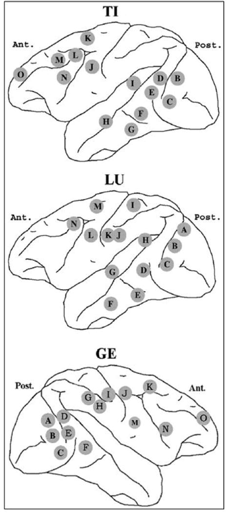
Top panel: schematic of electrode placement for monkey TI. Data from three prefrontal recording sites marked O, L, and M, referred to as PF1, PF2, and PF3 in the text, are further analyzed. Middle panel: schematic of electrode placement for monkey LU. Data from two recording sites marked K and L, which correspond to S1 and M1, are further analyzed. Bottom panel: schematic of electrode placement for monkey GE. Data from two recording sites marked I and J, which correspond to S1 and M1, are further analyzed.
In TI, the correct GO trials were rank ordered by RT and then sorted into groups of 200 trials each, starting with the fastest response times and proceeding to the slowest, each group sharing 150 trials with the previous one (Liang et al. 2002; Zhang et al. 2008). A total of 18 groups resulted. The mean RT for each group was calculated. Power spectrum and coherence were computed by fitting a MVAR (Ding et al. 2000) model to the LFPs from the ensemble of trials in each group during the 110ms pre-stimulus period (22 points for a sampling rate of 200 Hz). The main focus was the correlation between group mean RT and group power and coherence. The three recording sites, denoted PF1, PF2 and PF3, used for analysis were from the prefrontal cortex. Oscillatory activities in the beta frequency (14 to 30 Hz) range at these sites and their relation with the response time has been reported in the past (Liang et al. 2002; Zhang et al. 2008). Here our main interest includes this beta frequency band as well as the high gamma band which was defined to be from 60 to 90 Hz. Spearman rank correlation coefficients (SRCC) were computed for the relations of band-power and band-coherence with RT for both the noisy data and the signal after denoising.
The denoising algorithm yielded two time series: denoised signal and removed noise. To examine the issue of whether the removed noise is of a broadband nature we tested its whiteness according to the following procedure (Ding et al. 2000). For each of the three prefrontal data channels, we obtained time series of noise removed by the denoising algorithm. Auto and cross-correlations were computed up to lag 20, excluding lag 0, for all pairwise combinations of the above three noise time series. The null hypothesis was that the removed noise had no temporal correlation. For this to be true, more than 95% of the correlation coefficients were expected to fall within the interval (N denotes the number of time points in each trial which was 22 for this study). This allowed about 5% of the coefficients to fall outside the interval by pure chance even if the process was white.
In LU and GE, previous work has identified a beta oscillatory network in sensorimotor cortex during the prestimulus time period (Brovelli et al 2004; Zhang et al 2008). In particular, it was shown that the drive from the somatosensory site (S1) to the motor site (M1), denoted by S1→M1, is stronger than that in the opposite direction, denoted by M1→S1, in both monkeys. However, the ratio between these two Granger causal influences in the beta band, (S1→M1)/(M1→S1), which measures the input-output relationship at the involved cortical sites, is substantially different between the two monkeys. This inconsistency is hypothesized to be caused by noise. To test this hypothesis, we denoised the LFP data from both channels for both monkeys and subjected the denoised data again to Granger causality spectral analysis. The noise removed by the denoising algorithm was again examined for its broadband nature through whiteness test described in the preceding paragraph.
Results
Simulations
Example 1
We considered the following bivariate AR(2) process as a first test bed for our algorithm:
| (15) |
| (16) |
The values of the parameters used were a = 0.4, b = 0.6, d1 = 0.4, d2 = 0.5, and the covariance matrix S of the noise vector (ε1,ε2)′ is a diagonal matrix with entries 0.04 and 1.0. Two time series signals from channels z1 and z2 were generated by numerically simulating this MVAR model. A Gaussian measurement noise vector with a diagonal covariance matrix with entries 0.04 and 6.25 were added to the simulated data to create noisy data. It is clear that more noise was added to the signal from channel z2 than that from channel z1. In what follows we assumed that each time unit corresponded to 5ms and hence the sampling rate was 200 Hz. The data set consisted of 100 realizations, each of length 250 ms (50 points).
Assuming no knowledge of the generating model, the noisy data was denoised and smoothed by the denoising algorithm adapted to multiple trials. The power and coherence spectra were computed using the MVAR approach for both noisy data and denoised signal and are shown in Figure 2. Error bars for the coherence spectra were computed using the standard bootstrap procedure (Zoubir and Boashash B 1998). Several findings are noted. First, for channel z1, both noisy data and denoised signal have similar power spectra at all frequencies, in agreement with the exact power spectrum (Fig. 2; top panel). This is expected as this signal was relatively noise free. Second, for channel z2, the denoised signal has a power spectrum that is much closer to the exact spectrum (Fig. 2; middle panel), demonstrating the effectiveness of the denoising algorithm. Third, for channel z2, the signal to noise ratio becomes increasingly more unfavorable toward the higher end of the spectrum (Fig. 2; middle panel). Fourth, the coherence spectrum of the noisy data is greatly suppressed at higher frequencies due to the unfavorable signal to noise ratio (Fig. 2; bottom panel). However, after denoising, the coherence spectrum becomes much closer to the exact coherence spectrum (Fig. 2; bottom panel). This is again an illustration that the denoising algorithm can restore the statistical properties of the contaminated data.
FIG 2.

The power and coherence spectra of a noisy bivariate AR(2) process (example 1). The top and middle panels show the power spectra of channels z1 and z2, respectively. The solid lines depict the exact power spectra; the dotted lines indicate the power spectra of the noisy data; the dashed lines indicate the power spectra of the denoised signals; and the filled squares indicate the spectra for noise. The bottom panel represents the coherence spectra between z1 and z2. Here, the solid line indicates exact coherence spectrum; the dotted and dashed lines are the coherence spectra of noisy data and denoised signal, respectively. Error bars for the coherence spectra were computed using a bootstrap procedure. See text for more details.
Example 2
A bivariate AR(1) process as defined below was used for studying the effect of noise on Granger causality:
| (17) |
| (18) |
The parameter values used were a=0.4, b=0.6 and d=0.9 and the covariance matrix S of the noise vector (ε1,ε2)′ has diagonal entries 0.04 and 1.0 with off-diagonal entries both equal to 0.03. The nonzero off-diagonal entries imply that noise terms are correlated and this is one possible manifestation of a common unobserved input. We again obtained one hundred realizations of two time series signals from channels z1 and z2 by numerically simulating this MVAR model. Noisy data were created by adding Gaussian measurement noise with a diagonal covariance matrix whose entries were 0.04 and 6.25 to the simulated data. The duration of the signals was 250 ms (50 points) as in the previous example.
From the above AR(1) model, it is clear that channel z2 drives channel z1 and channel z1 does not drive channel z2. Hence, this is a unidirectional causal system by design. But on adding measurement noises to both channels, we observe that noisy z1 drives noisy z2, giving rise to spurious Granger causal direction as shown in Figure 3. Also, the true Granger causal direction is suppressed. Here, the solid lines represent the true Granger causality spectra, while the dotted lines represent the Granger causality spectra for noisy data. Error bars computed using a bootstrap procedure (Zoubir and Boashash B 1998) are also shown. On denoising the noisy data, we see that correct Granger causal directions are recovered and that the denoised spectra are reasonably close to the true Granger causality spectra. The dashed lines represent the Granger causality spectra for the denoised data.
FIG 3.

Granger causality spectra for data from a bivariate AR(1) process (example 2). The solid lines, dotted lines, dashed lines represent true Granger causality spectra from data without added noise, spectra from data with added noise, and spectra from the denoised data, respectively. Error bars were computed using a bootstrap procedure. Note that in the top panel the noise-free spectrum and the denoised spectrum nearly coincide.
Example 3
Consider again the model in Eqs. (17) and (18). It has been shown mathematically (Nalatore et al. 2007) that it is only the added noise in the driver channel (z2) that gives rise to spurious Granger causality. Hence, if z2 has no measurement noise, then no amount of added noise in the driven channel (z1) can lead to spurious Granger causality. On the other hand, as seen in Figure 3, a true Granger causal direction can be masked by added noise and the noise in both channels can contribute to this (Nalatore et al. 2007). Figure 4 demonstrates that spurious Granger causality is greatly diminished if driver channel (z2) has only a small amount of noise. All parameter values were taken to be the same as in Example 2 except that the measurement noise added to the driver channel z2 had variance 0.25 instead of 6.25.
FIG 4.

Granger causality spectra for data from a bivariate AR(1) process (example 3). The amount of noise added to the driver variable z2 is relatively small while the amount of noise added to the driven variable z1 is relatively large. The solid lines, dotted lines, dashed lines represent true Granger causality spectra from data without added noise, spectra from data with added noise, and spectra from the denoised data, respectively. Error bars were computed using a bootstrap procedure. Note that all three spectra in the top panel nearly coincide.
Experimental results
Dataset 1 (TI)
We apply the denoising algorithm (adapted to multiple trials) to the experimental data described in the Methods section for TI. Only the three prefrontal channels (PF1, PF2, and PF3; corresponding to recording sites O, L, and M respectively in top panel of Figure 1) were denoised. Figure 5 shows the power spectra for the noisy experimental data (dotted line), the denoised signal (dashed line), and removed noise (squares) for a single typical channel. Error bars computed using a bootstrap procedure (Zoubir and Boashash B 1998) are also shown. The noise is hypothesized to have a broadband spectrum. We applied the whiteness test to the noise, and the percentage of auto and cross-correlation coefficients that were outside the significance interval was below 2%, suggesting that the removed noise is indeed white. Figure 6 shows one realization of the removed noise as a function of time along with its autocorrelation function.
FIG 5.

The power spectra of the prestimulus data (-90 to 20 ms) at site PF3 for monkey TI. The dotted line, dashed line, and squares represent the power spectrum of the noisy data, the power spectrum of the denoised data, and the power spectrum of the removed noise, respectively. Error bars were computed using a bootstrap procedure.
FIG 6.

One realization of the removed noise as a function of time at site PF3 is shown in the top panel. The autocorrelation function is shown as a stem plot in the bottom panel. The horizontal dashed lines indicate the 95% confidence intervals for the process to be a white noise process.
The noisy data and the denoised signal have similar spectral features. A pronounced peak around 20 Hz indicates oscillatory activity in the beta range (Liang et al. 2002). The magnitude of power decreases rapidly as frequency increased past 40 Hz. While the amplitude of noise is small relative to the denoised signal in the lower frequency end of the spectrum, in the high gamma band, the noise is stronger than the signal. Table 1 summarizes the signal to noise ratio for the two frequency bands for all three channels. From the table it is reasonable to expect that noise has a much stronger impact on our analysis of neural activity in the high gamma band than that in the beta band. Consequently, denoising has the potential to reveal new physiological insights in high gamma band that were masked by noise in the original recording. This idea is tested below.
Table 1.
Signal to noise ratio (SNR) computed in the beta band (14 to 30 Hz) and high gamma band (60 to 90 Hz) for all three sites in monkey TI. See text for more details.
| Site | SNR in beta band (dB) | SNR in gamma band (dB) |
|---|---|---|
| PF1 | 8.9774 | -8.9911 |
| PF2 | 14.4898 | -0.6676 |
| PF3 | 12.5080 | -3.7906 |
Figure 7 shows the coherence between PF1 and PF2. Error bars were computed using a bootstrap procedure (Zoubir and Boashash B 1998). It can be seen that the coherence in the low frequency range stays roughly the same before and after the denoising operation, but the coherence from 60 to 90Hz increases 10 fold after noise is removed from the data. Substantial increases in coherence are found for other channel combinations. The ratios of coherence increase are summarized in the inset of Figure 7. Previous analysis of the same data reported (Liang et al. 2002; Zhang et al. 2008) that the power and coherence in the beta band is negatively correlated with the response time. Based on this finding it was hypothesized that beta oscillatory activity implemented anticipatory attention in the prefrontal cortex (Liang et al. 2002; Zhang et al. 2008). We repeated the same analysis here for the beta band activity using both the original noisy data and the denoised signal. From our earlier discussion, we expect the results to be similar in this low frequency range. The Spearman rank correlation coefficient (SRCC) was calculated to measure the correlation of pre-stimulus power and coherence peak values (in the beta frequency range) with response times. The values are shown in Tables 2 and 3. The peak power is significantly correlated (p < 0.01) with response time in all prefrontal sites for both noisy data and denoised signal. Similarly, peak coherence is also significantly correlated (p < 0.05) with response time for both noisy and denoised data for all site pairs. It is clear from Tables 2 and 3 that SRCC values stay essentially the same after denoising, confirming our expectation that the effect of noise is negligible in this case as a result of the large signal to noise ratio in this frequency range (Table 1).
FIG 7.

The coherence spectrum of the pre-stimulus data for prefrontal site pair PF1-PF2 of monkey TI. The dotted line and the dashed line represent the coherence of the noisy data and of the denoised data. Error bars were computed using a bootstrap procedure. Inset: The ratios of high gamma band coherence of denoised signal to that of noisy data are shown for all three site pairs with the plotted pair shaded.
Table 2.
Spearman rank correlation coefficient (SRCC) between peak power value in beta band and RT for the three sites in TI prefrontal cortex. The * denotes values that are significant at 1% level.
| Site | SRCC before denoising | SRCC after denoising |
|---|---|---|
| PF1 | -0.8246* | -0.8473* |
| PF2 | -0.6409* | -0.6759* |
| PF3 | -0.9133* | -0.8617* |
Table 3.
SRCC between peak coherence value in beta band and RT for site pairs in TI prefrontal cortex. The * denote values that are significant at 5% level.
| Site pair | SRCC before denoising | SRCC after denoising |
|---|---|---|
| PF1-PF2 | -0.4696* | -0.5624* |
| PF1-PF3 | -0.5851* | -0.6615* |
| PF2-PF3 | -0.5191* | -0.6594* |
Next, we consider the power and coherence in the high gamma band for the same recording channels (PF1, PF2 and PF3) and their correlation with RT. The results are shown in Table 4 and Figures 8-9. The SRCC of gamma band power is positive for all three sites and it is significant (p < 0.01) for PF2 (Table 4). The SRCC of gamma band coherence is significantly positive (p < 0.02) for all site pairs except PF1-PF3 (Figure 8). These results mean that the higher the synchronized high gamma activity in the prefrontal cortex the slower the response time. Such observations are at variance with the result obtained for the beta band and contradict the prior physiological findings that gamma activity is enhanced with the deployment of attention and increased attention led to faster response time (Womelsdorf et al. 2006).
Table 4.
SRCC between high gamma band power and RT for all three sites in TI prefrontal cortex before denoising. The * denotes values that are significant at 1% level.
| Site | SRCC before denoising |
|---|---|
| PF1 | 0.3478 |
| PF2 | 0.4489* |
| PF3 | 0.2157 |
FIG 8.

Scatter plot showing positive correlation between pre-stimulus prefrontal network coherence in the high gamma band (60 to 90 Hz) and RT for noisy data in monkey TI. Least-squares fit is superimposed. Inset: Spearman rank correlation coefficients between high gamma coherence and RT for all network site pairs are shown with the value for the plotted pair shaded.
FIG 9.

Scatter plot showing negative correlation between pre-stimulus prefrontal network coherence in the high gamma band and RT for denoised signal in monkey TI. A Least squares fit is superimposed. Inset: Spearman rank correlation coefficients between high gamma coherence and RT for all network site pairs are shown with the value for the plotted pair shaded.
Strikingly, after denoising, the high gamma band power and coherence for the denoised signal become negatively correlated with response time, as shown in Table 5 and Figure 9. Specifically, the negative value of SRCC for power is significant (p < 0.01) at site PF1 (Table 5), and the negative values of coherence are significant (p < 0.02) for all site pairs (Figure 9). These results, in conjunction with the signal to noise ratios reported in Table 1, suggest that the positive correlation observed for the noisy data in the high gamma frequency band is largely due to the effect of noise. It is worth noting that the result obtained by Womelsdorf et al. 2006 does not involve a denoising procedure.
Table 5.
SRCC between high gamma band power and RT for all three sites in TI prefrontal cortex after denoising. The * denotes values that significant at 1% level.
| Site | SRCC after denoising |
|---|---|
| PF1 | -0.6388* |
| PF2 | -0.2363 |
| PF3 | -0.1950 |
Dataset 2 (LU and GE)
We now study the Granger causal relations between one recording site in primary somatosensory cortex (S1) and another in primary motor cortex (M1) in monkeys LU and GE. These recording sites correspond to sites K and L respectively in Figure 1 (middle panel) for monkey LU and to sites I and J respectively for monkey GE (Figure 1; bottom panel). The LFP data for these two channels are denoised and Granger causal relations are computed for both the original noisy data and the denoised data. The results are shown in Figure 10 for LU and Figure 11 for GE, respectively. Error bars were computed using a bootstrap procedure (Zoubir and Boashash B 1998). In LU, it was found that the peak at 20Hz for the Granger causality in the direction S1→M1 is enhanced significantly after denoising (solid lines), whereas there is no major corresponding change for Granger causality in the opposite direction M1→S1. In the case of GE, Granger causality from M1 to S1 remains small after denoising, while for S1→M1, no significant change is observed (see Figure 11). The signal to noise ratio (SNR) was calculated over the frequency band 10-35 Hz for both monkeys and is shown in Table 6. From the table it is clear that the effect of noise should be more severe in LU than in GE.
FIG 10.

Granger causality spectra between sites S1 and M1 for monkey LU. The dashed lines and solid lines represent spectra for noisy data and denoised data respectively. Error bars were computed using a bootstrap procedure.
FIG 11.

Granger causality spectra between sites S1 and M1 for monkey GE. The dashed lines and solid lines represent spectra for noisy data and denoised data respectively. Error bars were computed using a bootstrap procedure.
Table 6.
SNR over the frequency band 10-35 Hz for monkeys LU and GE.
| Site name | LU SNR in dB | GE SNR in dB |
|---|---|---|
| M1 | 0.4686 | 11.7769 |
| S1 | 9.7053 | 8.0455 |
Band Granger causality, which was computed by summing the Granger causality spectrum over a narrow frequency range around the beta peak frequency, was evaluated for both noisy data and denoised data for both monkeys. In LU, the Granger causality spectra in the direction S1 →M1 has a peak at 20Hz and a 6 Hz band centered around this frequency was chosen. Likewise, in GE, a 6 Hz frequency band around 21 Hz was chosen. Each of these band Granger causality values are as shown in Tables 7 and 8 for LU and GE respectively. On taking the ratio of the above band Granger causality value in the direction S1→M1 to the band Granger causality value in the direction M1→S1, we found that this ratio was markedly different for both monkeys before denoising as shown in Figure 12. Error bars were computed using a bootstrap procedure (Zoubir and Boashash B 1998). Physiologically, this ratio is a measure of input-output relationship for the involved cortical site. The dramatic difference in this ratio between the two monkeys represents a discrepancy in this input-output relationship and the effect of noise is surmised. As expected, after denoising, the above described band Granger causality ratio is seen to be more consistent across the two monkeys, as shown in Figure 13.
Table 7.
Granger causality over a narrow frequency band around beta peak frequency for LU.
| S1→M1 | M1→S1 | |
|---|---|---|
| Before denoising | 0.6354 | 0.1467 |
| After denoising | 2.9890 | 0.1826 |
Table 8.
Granger causality over a narrow frequency band around beta peak frequency for GE.
| S1→M1 | M1→S1 | |
|---|---|---|
| Before denoising | 0.8100 | 0.0144 |
| After denoising | 1.2322 | 0.0572 |
FIG 12.

Ratio between S1→M1 and M1→S1 Granger causality in beta band for noisy data for monkeys LU and GE. Error bars were computed using a bootstrap procedure.
FIG 13.

Ratio between S1→M1 and M1→S1 Granger causality in beta band for denoised data for monkeys LU and GE. Error bars were computed using a bootstrap procedure.
Discussion and Summary
Neural noise refers to random activity in the nervous system that is not related to the processing of sensory input or motor output. The role of noise in neural information processing has been studied in the past. In coding theory, the rate coding hypothesis considers the variability in inter-spike intervals irrelevant noise, whereas for the temporal coding hypothesis, this variability is an important part of signal transmission (Stein et al. 2005). In sensory systems, it has been shown that the presence of noise can enhance the perception of weak coherent stimuli through the mechanism of stochastic resonance (Wiesenfeld and Moss 1995). Neural noise has also been implicated in age-related differences of cognitive functioning (Welford 1981; Cremer and Zeef 1987). Here, the slower information processing due to ageing is hypothesized to be caused by a lower signal-to-noise ratio which leads to higher sensory thresholds (Myerson 1990).
Electroneurophysiology gains insight into functions of the brain by relying on the statistical analysis of data collected in the form of time series. Given the complexity of the neural system these time series can be viewed as composed of two parts: signals of interest and other unrelated processes collectively referred to as noise. In this definition, the source of noise is manifold, including neural noise which is intrinsic to the nervous system, as well as environmental and instrumental noise. Unlike many previous reports, the focus of the present work is not on how noise affects neuronal information processing; instead we explore how the presence of noise impedes our ability to extract meaningful information from measurements via statistical analysis. This question has been considered extensively in the statistics literature (Fuller 1987). For example, it is known that linear regression, which is the basis for many statistical quantities, is highly vulnerable to noise contamination. Analyzing multivariate recordings with partial coherence, Albo et al. (2004) showed that signal to noise ratio is the key determinant in the identification of the generators of oscillatory activity in a network, irrespective of the true underlying connectivity pattern. Particularly significant for the analysis of neural data is the fact that the power of a neural signal decreases rapidly as the frequency increases into the gamma range (30 to 90 Hz) (1/f spectrum) (Buzsaki and Draguhn 2004). If the noise has a broadband spectrum, this means that the signal to noise ratio will become progressively more deteriorated in higher frequencies, limiting our ability to understand the true nature of neural activity in this frequency range. Despite such concerns, no attempts have been made to separate noise from signal, especially when the signal itself is a stochastic process occurring as the ongoing brain activity.
Our goal here is to apply a statistically principled method that can remove noise from noisy data to recover the signal of interest. The method is formulated in state space and based on the Kalman filter/smoother theory in conjunction with the Expectation-Maximization algorithm. To demonstrate the effectiveness of the method, we carried out simulation examples, where the noisy data were created by adding white Gaussian noise to the signal generated by a bivariate autoregressive process. In these examples, spectral properties of the signal were known a priori. We were thus able to verify that, whereas the added noise led to significantly distorted spectral properties, the procedure of denoising yielded markedly improved results.
Validating the denoising algorithm on actual neural data is a more challenging problem as there is no a priori information on signal or on noise. Knowledge from outside the analysis framework could help interpret the findings. Two LFP datasets from monkeys performing a visuomotor task were used for this purpose. The first dataset came from the prefrontal cortex of monkey TI. The second dataset consists of data from one somatosensory and one motor cortex site in two monkeys (LU and GE).
For the first dataset, the research question concerns how neural activity immediately preceding the onset of stimulus (prestimulus) was correlated with the response time (RT) (Liang et al. 2002; Zhang et al. 2008). This choice was based on several considerations. First, RT varies significantly from trial to trial. Spontaneous fluctuations of neural activity during the prestimulus time period in the prefrontal cortex reflect the level of anticipatory attention which inversely correlates with RT. Second, Liang et al. (2002) and Zhang et al. (2008) have analyzed the same data and observed the existence of a strong beta oscillatory network. The power and the coherence of this network is negatively correlated with RT. Third, oscillatory activity in the gamma range (30 to 90 Hz) is known to increase with the deployment of attention (Engel et al. 2001). In particular, Womelsdorf et al. (2006) reported that higher levels of gamma activity in visual cortex V4 is associated with faster RT in behaving monkeys. Given that the prefrontal cortex is the high center of executive control over the selection and coordination of processes in posterior cortical areas and that it is interconnected with V4, we expected that the gamma activity in the prefrontal cortex should be negatively correlated with RT. Fourth, as pointed out earlier, neural signal power is relatively weak in the gamma frequency range, making it vulnerable to the effect of noise. The denoising approach is best tested here as the result can be compared with the theoretical prediction. The application of the denoising algorithm leads to a removed noise time series and the denoised signal. The removed noise was shown to have a white spectrum. The signal to noise ratio was high in the beta range and very low in the high gamma range (60 to 90 Hz). The correlation between beta band activity and RT was not affected by the denoising operation, a consequence of the strong signal to noise ratio to begin with. In contrast, the gamma band power and coherence were found to be positively correlated with RT prior to denoising, meaning that higher the gamma activity slower the response time. After denoising, however, both power and coherence in the high gamma band became negatively correlated with RT, a finding in agreement with the theoretical prediction.
For the second dataset, the research question concerns the Granger causal influence in the beta frequency band between primary somatosensory (S1) and primary motor (M1) during the prestimulus time period. Based on the strong Granger causal influence from S1 to M1 as well as other evidence, Brovelli et al. (2004) proposed that the beta oscillatory network existed in support of sustained motor maintenance. When computing the ratio between Granger causal input and output of these sites, we found that this ratio is markedly different between the two monkeys. This discrepancy was thought to be caused by noise. In GE, the signal to noise ratio is relatively high at both recording sites. In LU, the site M1 had a high level of noise compared to site S1 (see Table 6). From Figure 10, it is clear that after denoising, the Granger causality in the direction S1→M1 is significantly enhanced, but there is no significant change in the Granger causality for the direction M1→S1. This can be understood as follows: our previous work has shown that (Nalatore et al. 2007) only noise in the driving channel contributes to spurious Granger causality (as also seen in Fig. 4 for the bivariate AR(1) model in simulation example 2). According to Brovelli et al. (2004), S1 is the driver of the network. Since the data from S1 have a small amount of noise, no significant spurious Granger causality from M1→S1 should be observed even for the original noisy data. It is thus not surprising that denoising has no effect on M1→S1. On the other hand, past work has also shown that noise in both channels contribute to suppression of true Granger causality (Nalatore et al. 2007). This is the reason why S1→M1 is so suppressed as a result of a large amount of noise in M1. Denoising significantly enhanced the true Granger causal influence. Importantly, the ratio between Granger causal input and output becomes more consistent across two monkeys after denoising, a result to be expected from the enhanced S1→M1 driving.
Brain activity in the absence of sensory stimulation is referred to as ongoing activity. Ongoing neural activity reflects important cognitive functions such as anticipation, attention and motor control. In this paper, we have modeled the ongoing neural data using an autoregressive plus additive white Gaussian noise model. In our experience, this model provides a good description for continuous-valued recordings such as local field potentials. Other types of linear models or even nonlinear models with non-Gaussian noise may also be considered. As our work is a proof of concept, the main goal is to establish that the denoising procedure based on a simple data model works on actual neural data. Our results provide support for this goal.
Acknowledgments
We thank Drs. Richard Nakamura, Richard Coppola and Steve Bressler for providing the data analyzed here. This work was supported by NIH grants MH71620, MH70498 and MH79388 and Air Force grant FA9550-07-1-0047. GR's work was supported in part by research grants from DRDO, DST (SR/S4/MS:419/07) and UGC-SAP (Phase IV). He is also associated with the Jawaharlal Nehru Centre for Advanced Scientific Research, Bangalore as an Honorary Faculty Member.
Appendix
In Kalman smoother, we perform both a forward pass and a backward pass on the data. The forward pass gives the usual Kalman filter equations:
| (A1) |
| (A2) |
| (A3) |
| (A4) |
starting with x̂1|0 = μ and P1|0 = V 1.
In the backward pass or the fixed interval smoothing part (Shumway and Stoffer 2000), we start with x̂T,PT and work backwards to update estimates of x̂t|T,Pt|T etc. One can show that we get the following equations (Gahramani and Hinton 1996):
| (A5) |
| (A6) |
| (A7) |
We also require Pt,t−1|T which can be written using the covariance smoothing algorithm (Shumway and Stoffer 2000) as Vt,t−1|T + x̂t|T (x̂t − t/T)′ where Vt,t−1|T is given by the backward recursion
| (A8) |
which is initialized using
| (A9) |
Footnotes
Publisher's Disclaimer: This is a PDF file of an unedited manuscript that has been accepted for publication. As a service to our customers we are providing this early version of the manuscript. The manuscript will undergo copyediting, typesetting, and review of the resulting proof before it is published in its final citable form. Please note that during the production process errors may be discovered which could affect the content, and all legal disclaimers that apply to the journal pertain.
References
- Albo Z, Viana Di Prisco G, Chen Y, Rangarajan G, Truccolo W, Feng J, Vertes RP, Ding M. Is partial coherence a viable technique for identifying generators of neural oscillations? Biol Cybern. 2004;90:318–26. doi: 10.1007/s00422-004-0475-5. [DOI] [PubMed] [Google Scholar]
- Bernasconi C, Konig P. On the directionality of cortical interactions studied by structural analysis of electrophysiological recordings. Biol Cybern. 1999;81:199–210. doi: 10.1007/s004220050556. [DOI] [PubMed] [Google Scholar]
- Bernasconi C, Von Stein A, Chiang C, Konig P. Bi-directional interactions between visual areas in the awake behaving cat. NeuroReport. 2000;11:689–92. doi: 10.1097/00001756-200003200-00007. [DOI] [PubMed] [Google Scholar]
- Bollimunta A, Chen Y, Schroeder CE, Ding M. Neuronal Mechanisms of cortical alpha oscillations in awake-behaving macaques. J Neurosci. 2008;28:9976–88. doi: 10.1523/JNEUROSCI.2699-08.2008. [DOI] [PMC free article] [PubMed] [Google Scholar]
- Bressler SL, Coppola R, Nakamura R. Episodic multiregional cortical coherence at multiple frequencies during visual task performance. Nature. 1993;366:153–56. doi: 10.1038/366153a0. [DOI] [PubMed] [Google Scholar]
- Brovelli A, Ding M, Ledberg A, Chen Y, Nakamura R, Bressler SL. Beta oscillations in a large-scale sensorimotor cortical network: Directional influences revealed by Granger causality. PNAS. 2004;101:9849–54. doi: 10.1073/pnas.0308538101. [DOI] [PMC free article] [PubMed] [Google Scholar]
- Buzsaki G, Draguhn A. Neuronal oscillations in cortical networks. Science. 2004;304(5679):1926–29. doi: 10.1126/science.1099745. [DOI] [PubMed] [Google Scholar]
- Chen Y, Bressler SL, Ding M. Frequency decomposition of conditional Granger causality and application to multivariate neural field potential data. J Neurosci Meth. 2006;150:228–37. doi: 10.1016/j.jneumeth.2005.06.011. [DOI] [PubMed] [Google Scholar]
- Cremer R, Zeef EJ. What kind of noise increases with age? J Gerontol. 1987;42(5):515–18. doi: 10.1093/geronj/42.5.515. [DOI] [PubMed] [Google Scholar]
- Dempster AP, Laird NM, Rubin DB. Maximum likelihood from incomplete data via the EM algorithm. J Roy Stat Soc. 1977;39:1–38. [Google Scholar]
- Dhamala M, Rangarajan G, Ding M. Estimating Granger causality from Fourier and wavelet transforms of time series data. Phys Rev Lett. 2008a;100:018701. doi: 10.1103/PhysRevLett.100.018701. [DOI] [PubMed] [Google Scholar]
- Dhamala M, Rangarajan G, Ding M. Analyzing information flow in brain networks with nonparametric Granger causality. NeuroImage. 2008b;41:354–62. doi: 10.1016/j.neuroimage.2008.02.020. [DOI] [PMC free article] [PubMed] [Google Scholar]
- Digalakis V, Rohlicek JR, Ostendorf M. ML Estimation of a stochastic linear system with the EM algorithm and it's applications to speech recognition. IEEE Trans Speech Audio Process. 1993;1:431–42. [Google Scholar]
- Ding M, Bressler SL, Yang W, Liang H. Short window spectral analysis of cortical event related potentials by adaptive multivariate autoregressive (AMVAR) modeling: Data processing, model validation and variability assessment. Biol Cybern. 2000;83:35–45. doi: 10.1007/s004229900137. [DOI] [PubMed] [Google Scholar]
- Ding M, Chen Y, Bressler SL. Granger causality: Basic theory and applications to Neuroscience. In: Schelter B, Winterhalder M, Timmer J, editors. Handbook of Time Series Analysis. Wiley-VCH Verlag; Berlin: 2006. pp. 437–60. [Google Scholar]
- Engel AK, Fries P, Singer W. Dynamic predictions: Oscillations and synchrony in top-down processing. Nat Rev Neurosci. 2001;2:704–16. doi: 10.1038/35094565. [DOI] [PubMed] [Google Scholar]
- Gahramani Z, Hinton GE. Switching state-space models. Department of Computer Science Technical Report, University of Toronto; 1996. [Google Scholar]
- Granger CWJ. Investigating causal relations by econometric methods and cross-spectral methods. Econometrica. 1969;37:424–38. [Google Scholar]
- Guo S, Seth AK, Kendrick KM, Zhou C, Feng J. Partial Granger causality— Eliminating exogenous inputs and latent variables. J Neurosci Meth. 2008;172:79–93. doi: 10.1016/j.jneumeth.2008.04.011. [DOI] [PubMed] [Google Scholar]
- Guo S, Wu J, Ding M, Feng J. Uncovering interactions in the frequency domain. PLoS Computat Biol. 2008;4:e1000087. doi: 10.1371/journal.pcbi.1000087. [DOI] [PMC free article] [PubMed] [Google Scholar]
- Fuller WA. Measurement Error Models. Wiley; 1987. [Google Scholar]
- Haykin S. Adaptive Filter Theory. Prentice Hall; 2001. [Google Scholar]
- Hesse W, Moller E, Arnold M, Schack B. The use of time-variant EEG Granger causality for inspecting directed interdependencies of neural assemblies. J Neurosci Meth. 2003;124:27–44. doi: 10.1016/s0165-0270(02)00366-7. [DOI] [PubMed] [Google Scholar]
- Keil A, Muller MM, Ray WJ, Gruber T, Elbert T. Human gamma band activity and perception of a gestalt. J Neurosci. 1999;19:7152–61. doi: 10.1523/JNEUROSCI.19-16-07152.1999. [DOI] [PMC free article] [PubMed] [Google Scholar]
- Kulkarni JE, Paninski L. Common-input models for multiple neural spike-train data. Netw Comput Neural Syst. 2007;18:375–407. doi: 10.1080/09548980701625173. [DOI] [PubMed] [Google Scholar]
- Ledberg A, Bressler SL, Ding MZ, et al. Large-scale visuomotor integration in the cerebral cortex. Cerebr Cortex. 2007;17:44–62. doi: 10.1093/cercor/bhj123. [DOI] [PubMed] [Google Scholar]
- Liang H, Bressler SL, Ding M, Truccolo WA, Nakamura R. Synchronized activity in prefrontal cortex during anticipation of visuomotor processing. NeuroReport. 2002;13:2011–15. doi: 10.1097/00001756-200211150-00004. [DOI] [PubMed] [Google Scholar]
- Marinazzo D, Pellicoro M, Stramaglia S. Kernel method for nonlinear Granger causality. Phys Rev Lett. 2008;100:144103. doi: 10.1103/PhysRevLett.100.144103. [DOI] [PubMed] [Google Scholar]
- Myerson J, Hale S, Wagstaff D, Poon LW, Smith GA. The information loss model: A mathematical theory of age related cognitive slowing. Psychol Rev. 1990;97:475–87. doi: 10.1037/0033-295x.97.4.475. [DOI] [PubMed] [Google Scholar]
- Nalatore H, Ding M, Rangarajan G. Mitigating the effects of measurement noise on Granger Causality. Phys Rev E. 2007;75:031123. doi: 10.1103/PhysRevE.75.031123. [DOI] [PubMed] [Google Scholar]
- Nykamp DQ. A mathematical framework for inferring connectivity in probabilistic neuronal networks. Math Biosci. 2007;205:204–51. doi: 10.1016/j.mbs.2006.08.020. [DOI] [PubMed] [Google Scholar]
- Nykamp DQ. Pinpointing connectivity despite hidden nodes within stimulus-driven networks. Phys Rev E. 2008;78:021902. doi: 10.1103/PhysRevE.78.021902. [DOI] [PubMed] [Google Scholar]
- Rajagovindan R, Ding M. Decomposing neural synchrony: Toward an explanation for near-zero phase-lag in cortical oscillatory networks. PLoS One. 2008;3:e3649. doi: 10.1371/journal.pone.0003649. [DOI] [PMC free article] [PubMed] [Google Scholar]
- Roweis S, Ghahramani Z. A unifying review of linear Gaussian models. Neural Comput. 1999;11:305–45. doi: 10.1162/089976699300016674. [DOI] [PubMed] [Google Scholar]
- Schnitzler A, Gross J. Normal and pathological oscillatory communication in the brain. Nat Rev Neurosci. 2005;6:285–96. doi: 10.1038/nrn1650. [DOI] [PubMed] [Google Scholar]
- Shumway RH, Stoffer DS. An approach to time series smoothing and forecasting using the EM algorithm. J Time Anal. 1982;3:253–64. [Google Scholar]
- Shumway RH, Stoffer DS. Time series analysis and its applications. Springer; 2000. [Google Scholar]
- Smith AC, Brown EN. Estimating a state-space model from point process observations. Neural Comput. 2003;24:447–61. doi: 10.1162/089976603765202622. [DOI] [PubMed] [Google Scholar]
- Smith AC, Frank LM, Wirth S, Yanike M, Hu D, Kubota Y, Graybiel AM, Suzuki W, Brown EN. Dynamic analysis of learning in behavioral experiments. J Neurosci. 2004;15:965–91. doi: 10.1523/JNEUROSCI.2908-03.2004. [DOI] [PMC free article] [PubMed] [Google Scholar]
- Smith AC, Stefani MR, Moghaddam B, Brown EN. Analysis and design of behavioral experiments to characterize population learning. J Neurophysiol. 2005;93:1776–92. doi: 10.1152/jn.00765.2004. [DOI] [PubMed] [Google Scholar]
- Stein RB, Gossen ER, Jones KE. Neuronal variability: Noise or part of the signal? Nat Neurosci. 2005;6:389–97. doi: 10.1038/nrn1668. [DOI] [PubMed] [Google Scholar]
- Tallon-Baudry C, Bertrand O. Oscillatory gamma activity in humans and its role in object representation. Trends Cognit Sci. 1999;3(4):151–62. doi: 10.1016/s1364-6613(99)01299-1. [DOI] [PubMed] [Google Scholar]
- Weinstein E, Oppenheim AV, Feder M, Buck JR. Iterative and sequential algorithms for multisensor signal enhancement. IEEE Trans Signal Process. 1994;42:846–59. [Google Scholar]
- Welford AT. Signal, noise, performance and age. Hum Factors. 1981;23:97–109. doi: 10.1177/001872088102300109. [DOI] [PubMed] [Google Scholar]
- Wiesenfeld K, Moss F. Stochastic Resonance and the benefits of noise: from ice ages to crayfish and squids. Nature. 1995;373:33–6. doi: 10.1038/373033a0. [DOI] [PubMed] [Google Scholar]
- Womelsdorf T, Fries P, Mitra PP, Desimone R. Gamma band synchronization in visual cortex predicts speed of change detection. Nature. 2006;439:733–36. doi: 10.1038/nature04258. [DOI] [PubMed] [Google Scholar]
- Zhang Y, Wang X, Bressler SL, Chen Y, Ding M. Prestimulus cortical activity is correlated with speed of visuomotor processing. J Cogn Neurosci. 2008;20:1915–25. doi: 10.1162/jocn.2008.20132. [DOI] [PubMed] [Google Scholar]
- Zhang Y, Chen Y, Bressler SL, Ding M. Response preparation and inhibition: The role of the cortical sensorimotor beta rhythm. Neurosci. 2008;156:238–46. doi: 10.1016/j.neuroscience.2008.06.061. [DOI] [PMC free article] [PubMed] [Google Scholar]
- Zoubir AM, Boashash B. The bootstrap and its application to signal processing. IEEE Signal Process Mag. 1998;15:56–76. [Google Scholar]