Abstract
The usefulness of fuzzy segmentation algorithms based on fuzzy connectedness principles has been established in numerous publications. New technologies are capable of producing larger-and-larger datasets and this causes the sequential implementations of fuzzy segmentation algorithms to be time-consuming. We have adapted a sequential fuzzy segmentation algorithm to multi-processor machines. We demonstrate the efficacy of such a distributed fuzzy segmentation algorithm by testing it with large datasets (of the order of 50 million points/voxels/items): a speed-up factor of approximately five over the sequential implementation seems to be the norm.
Keywords: Segmentation, Fuzzy Set Theory, Distributed Systems, Multi-Processor Computers
1 Introduction
Segmentation of an image (i.e., the process of separating, extracting, defining and/or labeling meaningful regions in an image) is an important process in many tasks in image processing, analysis and visualization, for example, in biology and medicine [23]. Humans have a powerful recognition and visual system that allows them to segment “well” an image under all kinds of conditions. Contrary to this, segmentation is a very challenging task for computers, and research in this field of computer science is prolific. Recently developed algorithms based on the concept of fuzzy connectedness have been shown to produce “good” results under various conditions of noise, texture and artifacts for a variety of imaging technologies [5, 7, 8, 11, 25]. Their applications include studies to segment automatically brain [28] and abdominal [29] MR images with the assistance of an atlas of their corresponding regions, to segment MR images even if corrupted by variation of the magnetic field [16], to segment vector-valued functions [11, 30], to detect and quantify multiple sclerosis in MR images [13, 24, 26], to segment images produced by PET [3], to analyze the morphology of airway tree structures [12, 15, 22] and to segment datasets in electron tomography [9].
Although the approach presented in this paper is quite general, our main motivation comes from imaging and this controls our terminology. In particular, we use the word spel (short for spatial element) to refer to points/voxels/items in a dataset. An imaging system will assign to all spels a value, the collection of spels with their associated values is referred to as an image.
The aim of fuzzy segmentation is to assign, for each object that is believed to be contained in the image and for any spel, a grade of membership of that spel in that object, whose value is a real number in the closed range between 0 (nonmembership) and 1 (full membership) [2, 18, 19, 27]. When using fuzzy connectedness to achieve this, we introduce, for each object that is believed to be contained in the image and for any pair of spels, a fuzzy spel affinity, whose value is also a real number in the closed range between 0 and 1. As presented in the next section, under some reasonable conditions, the set of fuzzy spel affinities will uniquely determine a set of grades of membership. The authors of [5] proposed an efficient sequential algorithm for obtaining these grades of membership from the fuzzy spel affinities: this algorithm produces a segmentation considerably faster than previous algorithms for doing such things, such as the one in [11].
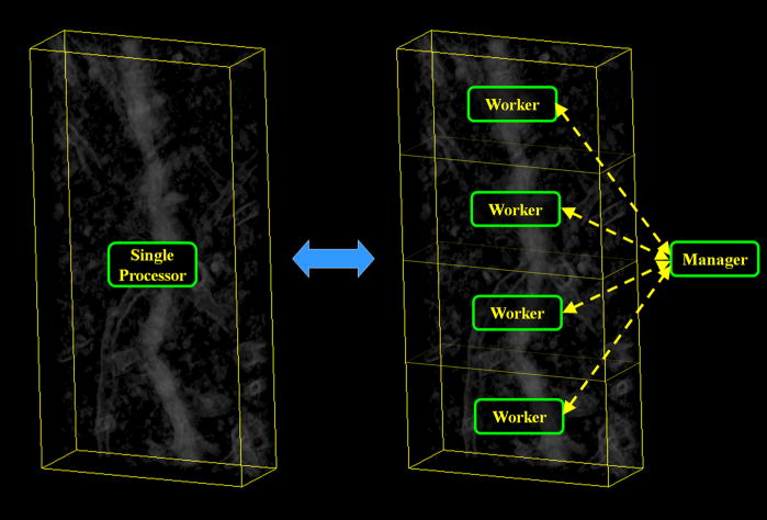
The fast algorithm proposed in [5] has been used to segment three-dimensional images produced by reconstruction algorithms from electron microscopic data (3DEM) of medium size biological specimens [9]. However, it may need over a quarter of an hour to process large specimens (consisting of over fifty million spels). Consequently, a further speed-up is desirable. To achieve this, we have adapted the algorithm in [5] to a distributed-processing scheme. The scheme that we followed is the so-called manager-worker (also known as master-slave), in which there are several processors (the workers) processing subsets of the dataset and there is a special processor (the manager) that controls how the other processors carry out the segmentation of their corresponding subset, see Figure 1.
Figure 1.
Scheme showing how a dataset that is originally processed by a single processor (left) can be divided into several smaller blocks and processed by several worker-processors controlled by a manager-processor (right).
In the next section we give a concise presentation of the existing theory behind the simultaneous segmentation of multiple objects and the efficient sequential algorithm proposed in [5]. In Section 3 we introduce the distributed version of this algorithm. Section 4 presents an implementation of the algorithm using OpenMP™ [6, 14] and its results using two multi-processor-shared-memory (MPSM) machines. Finally, we conclude in Section 5 with a discussion of our results.
2 Theory and Sequential Algorithm
In this section we give a concise, but mathematically complete, description of the theory behind the simultaneous segmentation of multiple objects and the efficient sequential algorithm proposed in [5]. Since we are not making any new contributions here, we keep this section as short as possible: we present only what is absolutely necessary to make our paper self-contained. For motivation, examples and explanations of the ideas that are introduced in the rest of this section, we refer the reader to [5] and its references.
Let V be an arbitrary nonempty finite set (its elements are the aforementioned spels) and let M be an arbitrary positive integer (the number of objects believed to be contained in the image). An M-semisegmentation of V is a function σ that maps each c ∈ V into a (M + 1)-dimensional vector , such that
,
for each m (1 ≤ m ≤ M), the value of is either 0 or , and
for at least one m (1 ≤ m ≤ M), .
We say that an M-semisegmentation σ is an M-segmentation if, for every spel c, is positive.
We call a sequence 〈c(0), ···, c(K)〉 of distinct spels a chain; its links are the ordered pairs (c(k−1), c(k)) of consecutive spels in the sequence. The ψ-strength of a link is provided by the appropriate value of a fuzzy spel affinity function ψ: V2 → [0, 1]. The ψ-strength of a chain is the ψ-strength of its weakest link; the ψ-strength of a chain with only one spel in it is 1 by definition. A set U(⊆V) is said to be ψ-connected if, for every pair of spels in U, there is a chain in U of positive ψ-strength from the first spel of the pair to the second.
An M-fuzzy graph is a pair (V,Ψ), where V is a nonempty finite set and Ψ = (ψ1,···, ψM) with ψm (for 1 ≤ m ≤ M) being a fuzzy spel affinity. A seeded M-fuzzy graph is a triple (V,Ψ, ) such that (V,Ψ) is an M-fuzzy graph and
  = (S1, ···, SM), where Sm ⊆ V for 1 ≤ m ≤ M. Such a seeded M-fuzzy graph is said to be connectable if
the set V is φΨ-connected, where φΨ(c, d) = min1≤m≤M ψm(c, d) for all c, d ∈ V, and
Sm ≠ ∅, for at least one m, 1 ≤ m ≤ M.
For an M-semisegmentation σ of V and for 1 ≤ m ≤ M, we define the chain 〈c(0), ···, c(K)〉 to be a σm-chain if , for 0 ≤ k ≤ K. Furthermore, for W ⊆ V and c ∈ V, we use μσ,m,W (c) to denote the maximal ψm-strength of a σm-chain from a spel in W to c. (This is 0 if there is no such chain.)
Theorem
If (V,Ψ, ) is a seeded M-fuzzy graph (where Ψ = (ψ1, ···, ψM) and
  = (S1, ···, SM)), then
-
there exists an M-semisegmentation σ of V with the following property: for every c ∈ V, if for 1 ≤ n ≤ M
(1) then for 1 ≤ m ≤ M
(2) this M-semisegmentation is unique; and
it is an M-segmentation, provided that (V,Ψ,
 ) is connectable.
This theorem is proved in [5].
Suppose now that the set of nonzero fuzzy spel affinities for a particular class of problems is always a subset of a fixed set A. Let K be the cardinality of the set A ∪ {1}, and let 1 = a1 > a2 > ··· > aK > 0 be the elements of A ∪ {1}. The following efficient sequential algorithm (proposed in [5] for finding, for a seeded M-fuzzy graph, the unique M-semisegmentation that satisfies (i) of the theorem above) makes use, for 1 ≤ m ≤ M and 1 ≤ k ≤ K, of sets of spels U[m][k]. We denote the M ×K table containing these sets by U.
3 Distributed Algorithm
A simple way to visualize how Algorithm 1 works is to picture several armies, one for each of the M objects, advancing and claiming parts of the image simultaneously. Hence, it is tempting to mimic this behavior with several processors, one for each army. However, such an approach would not be convenient, since in many practical applications there are only a few objects (e.g., two or three) and the gain due to work distribution would not be significant. Another approach partitions the dataset V into as many contiguous subsets as there are processors, and each processors applies Algorithm 1 to its own subset. Since Algorithm 1 passes information across subsets, this scheme makes it difficult to capture, without excessive communication between the processors, the “blocking” aspect of Algorithm 1. By this we mean that an army cannot march through a territory occupied by a stronger army to get to a place where it could win the battle since at that place the other army is weaker. To put this into the point of view of the defenders: they need to secure only their borders, in that way the enemy cannot get into the interior. This blocking is achieved by Algorithm 1 by looping through the k in a strict order (Step 10 onwards).
Algorithm 1.
The Fast Sequential Fuzzy Segmentation (FSFS) algorithm of [5].
| 1: | for c ∈ V do |
| 2: | for m ← 0 to M do |
| 3: | |
| 4: | for m ← 1 to M do |
| 5: | for k ← 1 to K do |
| 6: | U[m][k] ← ∅ |
| 7: | for c ∈ Sm do |
| 8: | |
| 9: | U[m][1] ← Sm |
| 10: | for k ← 1 to K do |
| 11: | for m ← 1 to M do |
| 12: | while U[m][k] ≠ ∅ do |
| 13: | remove a spel d from U[m][k] |
| 14: | |
| 15: | while C ≠ ∅ do |
| 16: | remove a spel c from C |
| 17: | t ←min(ak, ψm (d,c)) |
| 18: | if then do |
| 19: | remove c from each set in U that contains it |
| 20: | for n ←1 to M do |
| 21: | |
| 22: | |
| 23: | insert c into the set U[m][l], where l is the integer such that al = t |
As we mentioned in the Introduction, we follow a different approach that in fact partitions the dataset V into I subsets. However, instead of every available processor applying Algorithm 1 to a corresponding subset, all the processors, except for one, apply to one of the I subsets only the section of Algorithm 1 that searches for spels to occupy with strength k for a given army m (Step 11 onwards). The control over the change of strength k (Step 10) is left to a manager. Hence, there are I + 1 processors and we use P0 to refer to the manager and Pi, 1 ≤ i ≤ I, to refer to a worker. By following this approach, it is possible to take advantage of using more processors than objects and still achieve the “blocking” aspect of Algorithm 1.
In this approach, the manager is responsible for creating (based on the input seeded M-fuzzy graph (V,Ψ, )) I partial seeded M-fuzzy graphs (Vi,Ψ,
 i), for 1 ≤ i ≤ I, that the workers need to carry out their work. The partial seeded M-fuzzy graphs (Vi,Ψ,
 i) are obtained from the original seeded M-fuzzy graph (V,Ψ,
 ) by partitioning the domain set V into I nonoverlapping subsets (i.e., Vi ∩ Vj = ∅, for i ≠ j). Because the manager partitions the set V, the sets Sm (recall that Sm, for 1 ≤ m ≤ M, in
  is a subset of V) need to be partitioned appropriately; hence
  is divided into I entities
  i = (Si,1, ···, Si,M) such that, for 1 ≤ i ≤ I, and Si,m = Vi ∩Sm. Also note that the Ψ = (ψ1,···, ψM) is not distributed among the processors, each receives a copy of Ψ as part of the partial seeded M-fuzzy graph (Vi,Ψ,
 i). We also divide up the table U by maintaining for worker Pi a table Ui[m][k] = Vi ∩U[m][k].
Since the manager has control over the loop of Step 10 in Algorithm 1, a worker Pi needs to be continuously awaiting instructions from the manager to either initialize, or to carry out the Steps 11–23 of Algorithm 1, or to transfer back the local result to P0. Such communication takes place through an array of flags (one for each worker), named Signal, shared between P0 and the workers. The flags can take any of the values: Init, Process, Terminate and Finished. The last value is used by a worker to inform the manager that it has finished with a request. The first three values are used by the manager to inform a worker that it needs to carry out a given task; the manager assigns one of these values to the flag only if its current value is Finished. Moreover, the manager also informs workers of the level of strength k through a variable, named Strength, shared between P0 and the workers.
At a given level of strength k a processor Pi should carry out Steps 11–23 of Algorithm 1, but it may well occur that the information necessary to perform Step 14 is not available to the worker Pi, since some c may be a member of C due to a d ∈ Uj[m][k] with j ≠ i. The distributed version overcomes this problem by workers receiving information from other workers and transferring information to them through the manager. Such information is transferred by means of two arrays of queues  i and
i and  i for output and input, respectively. The queue Qi contains triples (d,c,m) in which d ∈ Ui [m][k] and c ∈ Vj for a j ≠ i with ψm (d,c) > 0. Conversely, the queue
  i contains triples (d,c,m) in which c ∈ Vi and d ∈ Uj [m][k] for a j ≠ i with ψm (d,c) > 0.
The partial seeded M-fuzzy graph (Vi,Ψ, i) is transferred to processor Pi during initialization, at which time the data structures U,
  and
and  for that processor are also initialized. The manager informs a worker that it needs to initialize by setting the appropriate flag in the array Signal to Init. Upon finishing the initialization, the worker sets its appropriate flag in the array Signal to Finished (see Steps 2–15 of Algorithm 2), at which point it is ready to work on its subset of V.
Algorithm 2.
Tasks performed by the worker processor Pi
| 1: | while Signali ≠ Terminate do |
| 2: | if Signali = Init then |
| 3: | retrieve (Vi,Ψ, i)
i) |
| 4: | for c ∈ Vi do |
| 5: | for m ← 0 to M do |
| 6: | |
| 7: | for m ← 1 to M do |
| 8: | for k ← 1 to K do |
| 9: | Ui[m][k] ← ∅ |
| 10: | for c ∈ Si,m do |
| 11: | |
| 12: | Ui[m][1] ← Si,m |
| 13: |  i ←
i ←  i ← ∅
i ← ∅ |
| 14: | Signali ← Finished |
| 15: | if Signali = Process then |
| 16: | k ← Strength |
| 17: | while  i ≠ ∅ do
|
| 18: | remove (d,c,m) from  i
i
|
| 19: | t ← min(ak,ψm (d,c)) |
| 20: | if and then do |
| 21: | if then do |
| 22: | remove c from each set in Ui that contains it |
| 23: | for n ← 1 to M do |
| 24: | |
| 25: | |
| 26: | insert c into the set Ui[m][l], where l is such that al = t |
| 27: | for m ← 1 to M do |
| 28: | while Ui[m][k] ≠ ∅ do |
| 29: | remove a spel d from the set Ui[m][k] |
| 30: | |
| 31: |  i =
i =  i ∪ {(d,c,m) | c ∈ Vj for j ≠ i and ψm (d,c) > 0
 |
| 32: | while C ≠ ∅ do |
| 33: | remove a spel c from C |
| 34: | t ←min(ak,ψm (d,c)) |
| 35: | if then do |
| 36: | remove c from each set in Ui that contains it |
| 37: | for n ← 1 to M do |
| 38: | |
| 39: | |
| 40: | insert c into the set Ui[m][l], where l is such that al = t |
| 41: | Signali ← Finished |
At every strength level k, the manager informs every worker that it needs to carry out work on its subset Vi by setting the variable Strength to k and the flags in Signal to Process. After receiving such a signal, the processor Pi performs work on the subset Vi that corresponds to Steps 11–23 of Algorithm 1. Upon finishing this work, the processor Pi lets the manager know that it has finished the work by setting the appropriate flag to Finished, see Steps 16–43 of Algorithm 2.
The tasks of the manager are described in Algorithm 3. Knowing the total number (I +1) of processors available, the manager produces from the input (V,Ψ, ) the I partial M-fuzzy graphs (Vi,Ψ,
 i) and signals to every worker Pi to initialize and then it waits until all the workers have finished their initialization stage; see Steps 1–5 of Algorithm 3.
Algorithm 3.
Tasks performed by the manager processor Po
| 1: | (I +1) ← number of processors available |
| 2: |
calculate (Vi,Ψ, i), for 1 ≤ i ≤ I
|
| 3: | for i ← 1 to I do |
| 4: | Signali ← Init |
| 5: | wait until Signali = Finished, for 1 ≤ i ≤ I |
| 6: | k = 1 |
| 7: | while k ≤ K do |
| 8: | Strength ← k |
| 9: | for i ← 1 to I do |
| 10: | Signali ← Process |
| 11: | wait until Signali = Finished, for 1 ≤ i ≤ I |
| 12: | for i ← 1 to I do |
| 13: | while Qi ≠ ∅ do |
| 14: | remove a (d,c,m) from Qi |
| 15: | if c ∈ Vj then insert (d,c,m) into  j
j
|
| 16: | if  i = ∅, for 1 ≤ i ≤ I, then k ← k +1
 |
| 17: | for i ← 1 to I do |
| 18: | Signali ← Terminate |
| 19: | combine the I partial M-semisegmentations into the final σ |
The manager needs to be certain that every worker has finished working on its corresponding partial seeded M-fuzzy graph before advancing to the next level of strength. After all the workers have finished their current process, Step 11, it is necessary to check whether they have transferred information by checking the status of the queues  i. When the manager encounters a non-empty queue
  i, it transfers the information to the appropriate input queue
  j, j ≠ i, Steps 12–15.
When the manager has finished looping through all the strength values k, it informs the workers that their job is done by setting all the flags in the array Signal to Terminate, Steps 17–18. The final result produced by the manager is the M-semisegmentation from the M-fuzzy graph (V,Ψ, ). However, the partition of the M-fuzzy graph into I partial M-fuzzy graphs results in the processor Pi producing σc only for c ∈ Vi. Consequently, upon termination the manager needs to fetch from the workers these I partial M-semisegmentations and produce the final M-semisegmentation σ, Step 19 of Algorithm 3.
4 Results
In order to test the distributed version of the Fast Sequential Fuzzy Segmentation (FSFS) algorithm, we used two multi-processor-shared-memory (MPSM) machines. This type of architecture can be implemented by gathering many processors in a single computer (a typical configuration found in traditional supercomputers) or by using many computers (i.e., nodes) that share their resources over a dedicated network (a configuration found in modern supercomputers). In our distributed version of the FSFS algorithm the transfer of information between workers and the manager is frequent. To reduce the communication overhead, it is desirable to carry out such transfers of information through variables stored in common main memory. We used two multi-processor computers, a Silicon Graphics Inc. Altix® that possesses twenty-four 64-bit Itanium® processors running at 1.5 GHz and has a total main memory of 23.6 Gbytes and a computer based on the Multi-Core Intel® technology that possesses two quad-core Xeon® E5430 processors running at 2.66 GHz (resulting in 8 processors) and has a total main memory of 8 Gbytes.
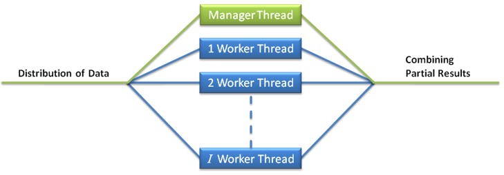
To take advantage of this computer architecture we used OpenMP™ [6, 14, 17]. OpenMP is an Application Program Interface (API) for multi-platform shared-memory parallel programming in C/C++ and FORTRAN. OpenMP is becoming the de facto standard for parallelizing applications for shared memory multiprocessors. An important advantage of OpenMP is that it is independent of the underlying hardware or operating system. The OpenMP API uses a fork-join model of parallel execution, see Fig. 2. In OpenMP, a program begins as a single thread of execution, called the initial thread. When any thread encounters a parallel construct, the thread creates a team of itself and additional threads and the original thread becomes the manager of this team. As for memory, OpenMP provides a relaxed-consistency, shared-memory model. All OpenMP threads have access to the memory. Importantly, each thread is allowed to have its own temporary view of the memory. However, OpenMP is capable of creating many threads inside a parallel construct, but these are not necessarily assigned to the same number of physical processors (i.e., multi-threading). Clearly, this behavior is undesirable for us, because many threads can overwhelm a processor and undermine its performance. Hence we made sure (by using features of OpenMP) that we never request more threads than the available physical processing units and that the threads are bound to physical processors.
Figure 2.
Scheme of the fork-join parallelism used by the distributed FSFS algorithm using OpenMP™. In Algorithm 3, distribution of data is done in Steps 1–5 and combining partial results is done in Step 19.
In order to test the performance of the implementation of the distributed FSFS algorithm, we used six images obtained by tomography of electron microscopic data. All of these datasets represent spiny dendrites [1, 21]. (Dendrites are the branch-like projections of a neuron whose function is to conduct the electrical signals received and processed by the neuron. Most principal neurons in the brain posses dendritic spines. These extend 1–2 microns from the shaft of the dendrite to make synapses with passing axons. A spiny dendrite makes synapses with a select few of the potential synaptic partners nearby.) For these tests M = 2: we refer to the object that contains voxels in the spiny dendrite as the foreground and the object that contains the rest of the voxels as the background. The images were obtained by using a reconstruction algorithm on a series of images acquired by tilting the specimen inside an Intermediate High Voltage Electron Microscope. The reconstruction assigns values υ(c) to the spels c ∈ V of an image whose spels are voxels arranged so that their centers form a portion of the simple cubic grid {(Δc1,Δc2,Δc3) | c1,c2,c3 ∈ ℤ} [11], see Table 1. We selected these datasets because they were large enough to make the implementation of the sequential FSFS algorithm use more than 5 minutes to process in a single-processor machine with 2 Gbytes of memory.
Table 1.
Dimensions of the images used for testing the distributed FSFS algorithm.
| Dataset | Dimensions (voxels) |
|---|---|
| A | 359 × 764 × 245 |
| B | 310 × 860 × 186 |
| C | 464 × 862 × 141 |
| D | 334 × 621 × 201 |
| E | 314 × 744 × 140 |
| F | 424 × 824 × 151 |
We consider the pair of voxels (c,d) to be face adjacent (notation: (c,d) ∈ ρ1) if the distance between their centers is equal to Δ and to be face-edge adjacent (notation: (c,d) ∈ ρ2) if the distance between their centers is less or equal to . As is common in practice (for geometrical reasons), for voxels in the foreground we use face adjacency and for voxels in the background we use face-edge adjacency [10].
The input seeded 2-fuzzy graphs (V, (ψ1,ψ2), (S1,S2)) to the algorithm were created as follows [4, 5, 11, 20]. A user, assisted with a graphical interface, selected seed voxels both for the foreground (S1) and the background (S2). The seed voxels and the voxels adjacent to them were used to estimate the means mi and standard deviations si of the sum (υ (c)+ υ (d)) and the means ni and standard deviations ti of the difference |υ (c) − υ (d)| for the two objects. Using these, we defined
| (3) |
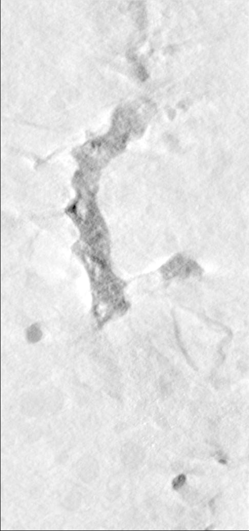
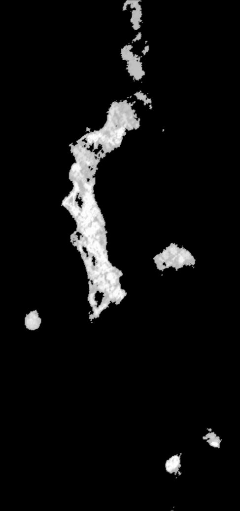
For the experiments we used different configurations, from 1 worker thread (equivalent to the sequential implementation of FSFS algorithm) up to seven worker threads for the Multi-Core Intel® computer and twenty-three worker threads for the Altix® computer. In order to verify that the distributed FSFS algorithm produces correct results, we compared the output produced by every configuration of the distributed FSFS algorithm with that produced by the sequential FSFS algorithm both visually, see Figure 3, and numerically (the outputs were identical voxel by voxel).
Figure 3.
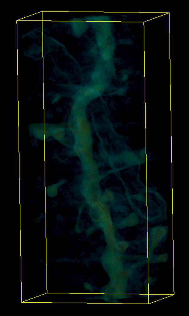

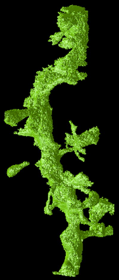
Visualizations of the output of the FSFS algorithm applied to dataset A. The upper row shows a single section of (a) the original 3D dataset, (b) output of the sequential and (c) distributed versions, respectively. The lower row shows a 3D representations of (d) the original dataset, (e) output of the sequential and (f) distributed versions of the FSFS algorithm (the latter images were produced by surface rendering the set of voxels ).
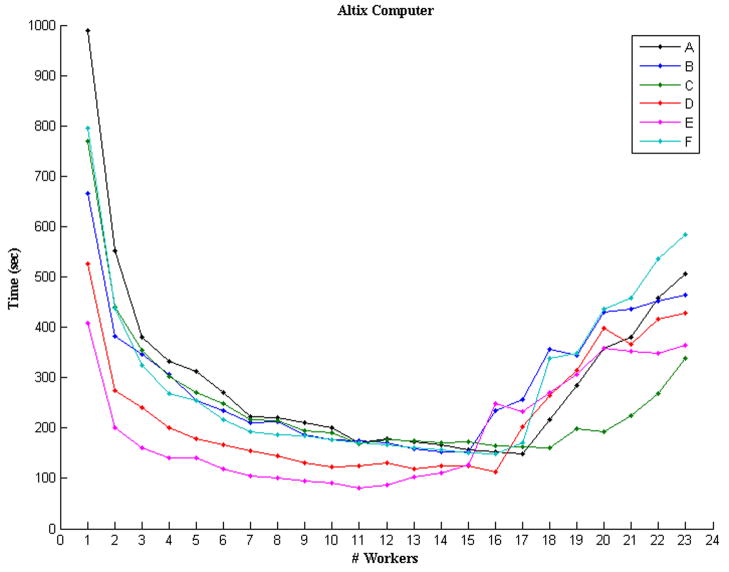
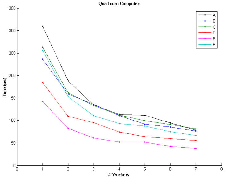
The program was executed ten times (with independently selected seed spels) for every one of the different configurations in order to obtain statistics of the execution times in seconds, see Tables 2 and 3 for the 24- and 8-processor machines, respectively. For visualization purposes only, we plotted the mean times of Tables 2 and 3 in Figure 4. From the plots, we can see that the behavior of the distributed program indeed improves in speed when the number of processors is increased, something that was expected. In the case of the Altix® computer, however, the performance starts to deteriorate at about 17 worker-processors. The reason for the reduction of speed at these configurations is due to the fact that the machine is shared by several users most of the time using anywhere from 6 to 8 processors constantly. Hence, using 16, or more, of the 24 processors forces the operating system to share the processors among jobs and the performance for each job deteriorates.
Table 2.
Time, in seconds, used by the distributed FSFS algorithm running on the Altix® computer for the six different images and various number of worker processors.
| Time (sec) | ||||||
|---|---|---|---|---|---|---|
| Dataset | ||||||
| No. Processors | A | B | C | D | E | F |
| 1 | 988.224±39.052 | 666.404±25.806 | 770.444±21.103 | 524.965±33.588 | 408.386±28.877 | 795.806±40.389 |
| 2 | 552.705±11.943 | 382.595±1.487 | 440.821±17.166 | 273.633±22.086 | 200.333±14.040 | 438.328±27.268 |
| 3 | 379.611±8.221 | 346.783±10.678 | 354.802±5.440 | 239.579±3.544 | 160.996±10.705 | 324.339±6.408 |
| 4 | 332.420±12.957 | 305.421±11.292 | 301.412±6.127 | 199.761±4.905 | 141.086±3.132 | 268.389±14.594 |
| 5 | 313.247±7.885 | 254.717±7.986 | 270.080±4.716 | 178.264±5.272 | 140.815±3.732 | 253.564±1.849 |
| 6 | 270.324±3.417 | 235.519±8.795 | 248.163±1.473 | 166.986±2.512 | 117.842±0.391 | 216.218±4.069 |
| 7 | 222.574±6.965 | 211.399±7.178 | 216.995±2.630 | 154.121±5.584 | 105.572±2.862 | 191.647±4.375 |
| 8 | 220.427±4.397 | 211.899±2.340 | 215.370±7.614 | 143.730±1.807 | 100.068±2.812 | 187.099±3.108 |
| 9 | 211.000±4.047 | 186.770±6.035 | 194.080±1.823 | 130.811±0.080 | 94.175±3.489 | 183.943±4.176 |
| 10 | 200.760±3.778 | 177.563±1.276 | 190.909±4.064 | 121.844±1.191 | 91.360±0.774 | 175.815±3.107 |
| 11 | 170.942±4.490 | 174.972±2.661 | 169.012±3.325 | 125.215±2.302 | 80.658±3.725 | 170.547±8.092 |
| 12 | 179.181±11.025 | 171.518±14.312 | 177.480±10.924 | 131.216±39.857 | 86.448±2.810 | 166.260±13.383 |
| 13 | 173.181±6.818 | 158.878±57.765 | 173.830563±14.234 | 119.574±26.731 | 103.555±17.454 | 161.169±20.394 |
| 14 | 165.977±7.512 | 152.737±16.892 | 169.846613±69.582 | 124.230±28.070 | 110.027±24.106 | 156.558±5.265 |
| 15 | 155.842±7.922 | 152.367±15.876 | 172.663858±54.061 | 123.896±41.582 | 126.788±73.099 | 150.925±32.335 |
| 16 | 152.894±57.230 | 234.613±51.083 | 165.169523±47.780 | 112.215±69.149 | 247.661±64.066 | 148.27±67.334 |
| 17 | 148.068±78.882 | 256.029±39.925 | 162.428771±49.703 | 202.534±63.485 | 232.109±10.649 | 170.169±39.115 |
| 18 | 215.894±72.108 | 355.918±79.708 | 160.600±74.245 | 265.466±40.200 | 269.698±18.826 | 338.270±33.597 |
| 19 | 284.302±56.912 | 343.974±25.898 | 198.860±45.111 | 314.029±69.670 | 305.991±12.420 | 348.807±5.261 |
| 20 | 357.806±42.606 | 429.281±30.850 | 192.410±53.219 | 397.407±40.703 | 357.943±29.001 | 436.986±19.960 |
| 21 | 379.991±58.168 | 437.029±37.402 | 225.405±68.874 | 365.813±52.541 | 353.186±11.183 | 458.093±54.959 |
| 22 | 458.394±37.195 | 452.292±58.730 | 267.468±39.558 | 416.879±40.389 | 347.493±11.824 | 535.998±26.707 |
| 23 | 505.802±65.719 | 465.035±51.146 | 338.667±18.841 | 427.284±27.295 | 365.187±10.339 | 582.990±19.686 |
Table 3.
Time, in seconds, used by the distributed FSFS algorithm running on the Multi-Core Intel® computer for the six different images and various number of worker processors.
| Time (sec) | ||||||
|---|---|---|---|---|---|---|
| Dataset | ||||||
| No. Processors | A | B | C | D | E | F |
| 1 | 310.115±0.117 | 236.753±0.147 | 262.690±0.959 | 184.586±0.085 | 142.013±0.768 | 255.999±0.150 |
| 2 | 188.558±3.422 | 158.622±2.701 | 161.537±2.098 | 109.502±2.120 | 82.483±1.306 | 152.704±2.074 |
| 3 | 134.570±1.078 | 135.592±0.627 | 132.917±0.828 | 95.147±0.682 | 61.474±0.590 | 110.714±1.150 |
| 4 | 113.728±0.850 | 110.977±0.350 | 111.987±0.377 | 74.210±0.236 | 52.123±0.312 | 92.930±0.497 |
| 5 | 111.379±0.937 | 92.156±0.824 | 99.833±0.434 | 63.909±0.602 | 52.359±0.143 | 87.349±0.341 |
| 6 | 94.941±1.291 | 85.243±0.713 | 91.004±1.191 | 59.958±0.506 | 42.542±0.572 | 75.185±1.008 |
| 7 | 78.313±1.148 | 76.504±0.343 | 81.179±0.967 | 55.877±0.434 | 38.167±0.310 | 66.755±0.289 |
Figure 4.
Plots showing the average times that (a) the Altixreg; computer and (b) the Multi-Core Intel® computer took to process the six datasets in Table 1.
Although the speed of the algorithm was, and is, our main interest, we also had the opportunity of observing the behavior of the maximum amount of main memory used by the implementation of the distributed FSFS algorithm in both computers. The total main memory in the computers we used for the experiments allows us to run the aforementioned datasets without the need of using virtual memory. Tables 4 and 5 show the maximum amount of memory (in Mbytes) utilized by each configuration in both computers. In general, the maximum amount of memory used by the distributed program diminishes when worker processors are used. Such a behavior is explained by how the distributed algorithm works: the way spels inserted into and are removed from the U arrays makes it likely that the maximum memory that is needed at any one time to store all the Ui is less than that needed to store the U in the sequential algorithm.
Table 4.
Maximum amount of memory used by both the sequential FSFS and the distributed FSFS algorithms when processing the six different datasets in the Altix® computer.
| Memory (Mbytes) | ||||||
|---|---|---|---|---|---|---|
| Dataset | ||||||
| No. Processors | A | B | C | D | E | F |
| 1 | 3,148.00 | 1,759.00 | 2,715.00 | 1,837.00 | 1,630.00 | 2,329.00 |
| 2 | 2,909.00 | 1,635.00 | 2,537.00 | 1,709.00 | 1,521.00 | 2,155.00 |
| 3 | 2,824.00 | 1,616.00 | 2,474.00 | 1,712.00 | 1,480.00 | 2,121.00 |
| 4 | 2,809.00 | 1,517.00 | 2,452.00 | 1,656.00 | 1,477.00 | 2,096.00 |
| 5 | 2,760.00 | 1,519.00 | 2,460.00 | 1,616.00 | 1,476.00 | 2,061.00 |
| 6 | 2,730.00 | 1,456.00 | 2,378.00 | 1,594.00 | 1,433.00 | 2,015.00 |
| 7 | 2,752.00 | 1,490.00 | 2,380.00 | 1,578.00 | 1,435.00 | 2,012.00 |
| 8 | 2,740.00 | 1,459.00 | 2,367.00 | 1,574.00 | 1,419.00 | 1,995.00 |
| 9 | 2,707.00 | 1,448.00 | 2,372.00 | 1,560.00 | 1,417.00 | 2,005.00 |
| 10 | 2,694.00 | 1,451.00 | 2,380.00 | 1,581.00 | 1,414.00 | 2,008.00 |
| 11 | 2,701.00 | 1,446.00 | 2,346.00 | 1,565.00 | 1,411.00 | 1,974.00 |
| 12 | 2,706.00 | 1,437.00 | 2,371.00 | 1,569.00 | 1,409.00 | 1,979.00 |
| 13 | 2,688.00 | 1,432.00 | 2,344.00 | 1,558.00 | 1,414.00 | 1,980.00 |
| 14 | 2,682.00 | 1,443.00 | 2,397.00 | 1,563.00 | 1,414.00 | 1,994.00 |
| 15 | 2,681.00 | 1,440.00 | 2,374.00 | 1,574.00 | 1,406.00 | 1,998.00 |
| 16 | 2,704.00 | 1,452.00 | 2,362.00 | 1,567.00 | 1,410.00 | 1,975.00 |
| 17 | 2,680.00 | 1,422.00 | 2,333.00 | 1,562.00 | 1,406.00 | 1,977.00 |
| 18 | 2,689.00 | 1,448.00 | 2,342.00 | 1,552.00 | 1,410.00 | 1,986.00 |
| 19 | 2,704.00 | 1,430.00 | 2,341.00 | 1,561.00 | 1,417.00 | 1,977.00 |
| 20 | 2,681.00 | 1,464.00 | 2,373.00 | 1,570.00 | 1,408.00 | 1,996.00 |
| 21 | 2,675.00 | 1,440.00 | 2,391.00 | 1,558.00 | 1,415.00 | 1,988.00 |
| 22 | 2,687.00 | 1,437.00 | 2,343.00 | 1,560.00 | 1,406.00 | 1,967.00 |
| 23 | 2,709.00 | 1,428.00 | 2,340.00 | 1,554.00 | 1,416.00 | 1,967.00 |
Table 5.
Maximum amount of memory used by both the sequential FSFS and the distributed FSFS algorithms when processing the six different datasets in the Multi-Core Intel® computer.
| Memory (Mbytes) | ||||||
|---|---|---|---|---|---|---|
| Dataset | ||||||
| No. Processors | A | B | C | D | E | F |
| 1 | 1,887.00 | 1,054.00 | 1,628.00 | 1,101.00 | 977.00 | 1,397.00 |
| 2 | 1,768.00 | 974.00 | 1,534.00 | 1,036.00 | 916.00 | 1,303.00 |
| 3 | 1,720.00 | 980.00 | 1,503.00 | 1,011.00 | 894.00 | 1,279.00 |
| 4 | 1,701.00 | 936.00 | 1,494.00 | 993.00 | 886.00 | 1,253.00 |
| 5 | 1,692.00 | 933.00 | 1,504.00 | 1,001.00 | 896.00 | 1,263.00 |
| 6 | 1,702.00 | 906.00 | 1,467.00 | 978.00 | 881.00 | 1,244.00 |
| 7 | 1,692.00 | 917.00 | 1,462.00 | 971.00 | 876.00 | 1,234.00 |
5 Discussion
There has been an immense effort by the computer science and engineering communities to produce semi-automatic and automatic segmentation algorithms. An important requisite for such algorithms is that they produce their results in nearly interactive time. Recently, algorithms have been developed based on the concept of fuzzy connectedness that produce “good” results under various conditions of noise, texture and artifacts for a variety of imaging technologies. In particular, the authors in [5] have proposed an algorithm (FSFS) that speeds up the performance of the Multi-Object Fuzzy Segmentation algorithm proposed in [11]. However, new imaging technologies are capable of producing very large datasets, and even the (sequential) FSFS algorithm takes a considerable amount of time to segment some of these datasets. Hence, we devised a distributed version of the FSFS algorithm that further improves its performance.
The distributed FSFS algorithm is designed for use on a multi-processor system, such as a multi-processor-shared-memory machine. Such machines are common among supercomputers. Typically, they are specialized computers that tend to be expensive. However, the trend of recent years is that even desktop computers come equipped with multi-core processors; with two cores being the most common nowadays. But, processor companies such as Intel® have introduced quad-core processors allowing computer manufacturers to offer multi dual- or quad-core processors. This means that in practice it is now possible to have multi-processor-shared-memory computers on desks. Taking advantage of such configurations is desirable for computing-intensive tasks, such as fuzzy segmentation.
In our approach, we used a manager that does not allow to move to a next level of strength until after all the workers have finished their work at the current level of strength. This approach can be further improved by doing a kind of “lookahead”; but that is more complex and needs more memory and so we left it to be a matter of future research.
Acknowledgments
The authors want to thank Stuart W. Rowland for his valuable comments and the Supercomputing Center of the D.G.S.C.A. at the U.N.A.M. for allowing the use of their facilities.
Footnotes
This work is supported in part by the National Institutes of Health (NIH) by Grant Number HL70472, by the DGAPA-UNAM under Grant IN98054 and by a grant of the CONACyT, Mexico.
References
- 1.Andersen P. Neurobiology - A spine to remember. Nature. 1999;399:19–21. doi: 10.1038/19857. [DOI] [PubMed] [Google Scholar]
- 2.Bandemer H, Gottwald S. Fuzzy Sets, Fuzzy Logic, Fuzzy Methods with Applications. Wiley; Chichester: 1995. [Google Scholar]
- 3.Carvalho BM, Garduño E, Herman GT. Multiseeded fuzzy segmentation on the face centered cubic grid. ICAPR ’01: Proceedings of the Second International Conference on Advances in Pattern Recognition; London, UK. Springer-Verlag; 2001. pp. 339–348. [Google Scholar]
- 4.Carvalho BM, Gau CJ, Herman GT, Kong TY. Algorithms for fuzzy segmentation. Pattern Analysis and Applications. 1999;2:73–81. [Google Scholar]
- 5.Carvalho BM, Herman GT, Kong TY. Simultaneous fuzzy segmentation of multiple objects. Discrete Applied Mathematics. 2005;151:55–77. [Google Scholar]
- 6.Chandra R, Menon R, Dagum L, Kohr D, Maydan D, McDonald J. Parallel programming in OpenMP. Morgan Kaufmann; San Francisco: 2000. [Google Scholar]
- 7.Ciesielskia KC, Udupa JK, Saha PK, Zhuge Y. Iterative relative fuzzy connectedness for multiple objects with multiple seeds. Computer Vision and Image Understanding. 2007;107:160–182. doi: 10.1016/j.cviu.2006.10.005. [DOI] [PMC free article] [PubMed] [Google Scholar]
- 8.Dellepiane SG, Fontana F, Vernazza GL. Nonlinear image labeling for multivalued segmentation. IEEE Transactions on Image Processing. 1996;5:429–446. doi: 10.1109/83.491317. [DOI] [PubMed] [Google Scholar]
- 9.Garduño E, Wong-Barnum M, Volkmann N, Ellisman M. Segmentation of electron tomographic data sets using fuzzy set theory principles. Journal of Structural Biology. 2008 doi: 10.1016/j-jsb.2008.01.017. [DOI] [PMC free article] [PubMed] [Google Scholar]
- 10.Herman GT. Geometry of Digital Spaces. Birkhäuser; Boston: 1998. [Google Scholar]
- 11.Herman GT, Carvalho BM. Multiseeded segmentation using fuzzy connectedness. IEEE Transactions on Pattern Analysis and Machine Intelligence. 2001;23:460–474. [Google Scholar]
- 12.Liu J, Udupa JK, Odhner D, McDonough JM, Arens R. System for upper airway segmentation and measurement with MR imaging and fuzzy connectedness. Academic Radiology. 2003;10:13–24. doi: 10.1016/s1076-6332(03)80783-3. [DOI] [PubMed] [Google Scholar]
- 13.Nyúl LG, Udupa JK. MR image analysis in multiple sclerosis. Neuroimaging Clinics of North America. 2000;10:799–815. [PubMed] [Google Scholar]
- 14.OpenMP Architecture Review Board, OpenMP application program interface version 2.5, tech. report, OpenMP Architecture Review Board, 2005.
- 15.Palágyi K, Tschirren J, Hoffman EA, Sonka M. Quantitative analysis of pulmonary airway tree structures. Computers in Biology and Medicine. 2006;36:974–996. doi: 10.1016/j.compbiomed.2005.05.004. [DOI] [PubMed] [Google Scholar]
- 16.Pednekar AS, Kakadiaris IA. Image segmentation based on fuzzy connectedness using dynamic weights. IEEE Transactions on Image Processing. 2006;15:1555–1562. doi: 10.1109/tip.2006.871165. [DOI] [PubMed] [Google Scholar]
- 17.Quinn MJ. Parallel Programming in C with MPI and OpenMP. McGraw-Hill Education Group; 2004. [Google Scholar]
- 18.Rosenfeld A. Fuzzy digital topology. Information and Control. 1979;40:76–87. [Google Scholar]
- 19.Rosenfeld A. On connectivity properties of greyscale pictures. Pattern Recognition. 1983;16:47–50. [Google Scholar]
- 20.Saha PK, Udupa JK, Odhner D. Scale-based fuzzy connected image segmentation: Theory, algorithms, and validation. Computer Vision and Image Understanding. 2000;77:145–174. [Google Scholar]
- 21.Sosinsky G, Martone ME. Imaging of big and messy biological structures using electron tomography. Microscopy Today. 2003;11:8–14. [Google Scholar]
- 22.Tschirren J, Hoffman EA, McLennan G, Sonka M. Intrathoracic airway trees: Segmentation and airway morphology analysis from low-dose CT scans. IEEE Transactions on Medical Imaging. 2005;24:1529–1539. doi: 10.1109/TMI.2005.857654. [DOI] [PMC free article] [PubMed] [Google Scholar]
- 23.Udupa JK, Herman GT. 3D Imaging in Medicine. 2. CRC Press, Inc.; Boca Raton, Florida: 1999. [Google Scholar]
- 24.Udupa JK, Nyul LG, Ge YL, Grossman RI. Multiprotocol MR image segmentation in multiple sclerosis: Experience with over 1,000 studies. Academic Radiology. 2001;8:1116–1126. doi: 10.1016/S1076-6332(03)80723-7. [DOI] [PubMed] [Google Scholar]
- 25.Udupa JK, Saha PK. Fuzzy connectedness and image segmentation. Proceedings of the IEEE. 2003;91:1649–1669. [Google Scholar]
- 26.Udupa JK, Wei L, Samarasekera S, Miki Y, van Buchem A, Grossman RI. Multiple sclerosis lesion quantification using fuzzy-connectedness principles. IEEE Transactions on Medical Imaging. 1997;16:598–609. doi: 10.1109/42.640750. [DOI] [PubMed] [Google Scholar]
- 27.Zadeh LA. Fuzzy sets. Information and Control. 1965;8:338–353. [Google Scholar]
- 28.Zhou Y, Bai J. Atlas-based fuzzy connectedness segmentation and intensity nonuniformity correction applied to brain MRI. IEEE Transactions on Biomedical Engineering. 2007;54:122–129. doi: 10.1109/TBME.2006.884645. [DOI] [PubMed] [Google Scholar]
- 29.Zhou Y, Bai J. Multiple abdominal organ segmentation: an atlas-based fuzzy connectedness approach. IEEE Transactions on Information Technology and Biomedicine. 2007;11:348–352. doi: 10.1109/titb.2007.892695. [DOI] [PubMed] [Google Scholar]
- 30.Zhuge Y, Udupa JK, Saha PK. Vectorial scale-based fuzzy-connected image segmentation. Computer Vision and Image Understanding. 2006;101:177–193. [Google Scholar]


