Relationship Between Adapted Neural Population Responses in MT and Motion Adaptation in Speed and Direction of Smooth-Pursuit Eye Movements

Abstract

We have asked how sensory adaptation is represented in the response of a population of visual motion neurons and whether the neural adaptation could drive behavioral adaptation. Our approach was to evaluate the effects of about 10 s of motion adaptation on both smooth-pursuit eye movements and the responses of neuron populations in extrastriate middle temporal visual area (MT) in awake monkeys. Stimuli for neural recordings consisted of patches of 100% correlated dot textures. There was a wide range of effects across neurons, but on average adaptation reduced the amplitude and width of the direction tuning curves of MT neurons, without large changes in the preferred direction. The effects were greatest when the direction of the adapting stimulus corresponded to the preferred direction of the MT neuron under study. Adaptation also reduced the amplitude of speed-tuning curves, again with the greatest effect when the adapting speed was equal to the preferred speed. The adapted tuning curves were shifted toward lower preferred speeds as the adapting speed increased. We constructed populations of model MT neurons based on our experimental sample and showed that the effects of adaptation on the direction and speed of pursuit eye movements were predicted when a variant of vector averaging decoded the responses of a subset of the neural population. We conclude that the effects of motion adaptation on the responses of MT neurons can support behavioral adaptation in pursuit eye movements.

INTRODUCTION

Both neuronal responses and behavior are subject to a process known as adaptation, which alters responses on the basis of the past history of sensory stimulation. Although there have been many demonstrations of neural and behavioral adaptation, one of the biggest unanswered questions is the relationship between adaptations of a neural population response and a quantifiable behavior. Can adaptation of the neural population responses drive the behavioral adaptation and, if so, how are the adapted responses of a population of neurons pooled, or decoded, to create behavioral adaptation (Kohn 2007)? Given that adaptation is more likely to alter sensory responses than to change decoding computations, understanding population decoding for adapted behavior would also illuminate how sensory population responses are decoded to drive normal behavior.

We have been addressing the neural basis for behavioral adaptation through a motor homologue to a well-known perceptual adaptation of the direction of motion (Levinson and Sekuler 1976; Schrater and Simoncelli 1998). Suppose a subject views an adapting stimulus that is moving to the right and reports the subjective direction of motion of subsequent probe stimuli that move to the right with an upward or downward component. After adaptation, the perceived direction of a probe stimulus is repelled from the adapting direction so that it is perceived to move more upward or downward than prior to adaptation. Gardner et al. (2004) demonstrated that the same directional adaptation occurs in smooth-pursuit eye movements.

Although expressed in a motor behavior, the directional adaptation of pursuit probably results from changes in the responses of visual neurons. The locus of adaptation cannot be in the motor system because it is dependent on the location of the test stimulus in the visual field; for a given direction of probe target motion, adaptation is expressed most strongly when the probe stimulus is presented in the same visual field location as the adapting stimulus; adaptation is not expressed at all when the probe and adapting stimuli are in opposite hemifields (Gardner et al. 2004). Further, the emergence of the same directional adaptation in both motor control and perception suggests a single common site of adaptation early in the motion-processing pathways. The middle temporal visual area (MT) seems like an excellent candidate as the locus of adaptation. Neurons in MT provide visual inputs for the perception of motion (Newsome et al. 1989; Salzman et al. 1992) and the initiation of smooth-pursuit eye movements (Born et al. 2000; Newsome et al. 1985). There have been abundant demonstrations of neural adaptation in MT (Kohn and Movshon 2003, 2004; Krekelberg et al. 2006; Peterson et al. 1985; van Wezel and Britten 2002), but our understanding of the links from neural to behavioral adaptation remains incomplete.

Previous work on visual population decoding has suggested pooling operations that could use the population response in MT to control pursuit eye movements or perception, with and without motion adaptation (Churchland and Lisberger 2001; Jazayeri and Movshon 2006; Kohn and Movshon 2004; Priebe and Lisberger 2004). We have now explored the neural and behavioral characteristics of a broader set of visual motion adaptations than studied in prior reports. We have used neural data recorded in monkeys to reconstruct most of the features of the motion adaptation recorded in pursuit direction and speed of the same species. The successful decoding computation implemented a variant of vector averaging while also converting the sensory population response into motor coordinates. By recording and quantitatively comparing neural and behavioral responses from the same species, our results move us closer to understanding both population decoding and the neural basis for behavioral adaptation.

METHODS

We conducted behavioral and neural adaptation experiments on two male rhesus monkeys that weighed 11 and 13 kg, plus behavioral adaptation experiments on two additional monkeys that weighed 9 and 15 kg. The monkeys had been trained to sit in a primate chair, with their heads secured to the ceiling of the chair, and to fixate and track targets presented on a video screen in front of them. Before experiments began, we conducted three sterile surgeries with the monkey under general anesthesia with isoflurane to implant 1) a head holder on the skull, 2) a scleral search coil in one eye, and 3) a recording cylinder. All methods had received prior approval from the Institutional Animal Care and Use Committee at UCSF and conformed to the National Institutes of Health Guide for the Care and Use of Laboratory Animals. Behavioral training, general experimental procedures, and surgical procedures were described in detail previously (e.g., Churchland and Lisberger 2001; Ramachandran and Lisberger 2005).

Visual stimuli

Visual stimuli consisted of single spots or patches of 100% correlated random dots displayed on an analog oscilloscope that was placed 23 cm from the monkey and subtended horizontal and vertical angles of 61 and 49°. The spot size was 0.1 × 0.1° and consisted of multiple closely spaced dots with a total luminance of 10.2 cd/m²; the patch size varied from 2 × 2° to 15 × 15° depending on the experiments. The dot density was 0.6 dot/deg² for physiology experiments and 1.2 dots/deg² for behavioral experiments. Each dot had a luminance of 1.7 cd/m². All experiments were conducted in a reasonably dark room with the main source of illumination coming from the dark gray screen of the display oscilloscope. The D/A converters from a digital signal processing (DSP) board in our experimental-control computer drove the analog display scope: spatial resolution was based on 65,536 (2¹⁶) pixels across the screen, individual dots appeared with a temporal interval of 10 μs, and the refresh rate for the full visual display was 4 ms. The speed of the DSP board limited the number of dots we could paint in a single refresh of the screen, explaining why we used lower dot densities for physiology experiments, when the visual stimulus might be as large as 225 deg². We will show that the behavioral adaptation does not depend consistently on the form or size of the stimulus, suggesting that differences in the form of the visual stimulus across our experiments are minor and will not affect our conclusions.

Recording procedures

Eye position and velocity were recorded with 1-ms temporal resolution using a scleral search coil. Eye velocity records were obtained by running the eye position signals through an analog circuit that differentiated signals at frequencies <25 Hz and rejected signals at higher frequencies.

We made extracellular recordings from single MT neurons with platinum/tungsten electrodes (2–4 MΩ; Thomas Recording, Giessen, Germany). Recordings were amplified, band-pass filtered (400 Hz to 8 kHz), and digitized for subsequent analysis. Single units were identified with a real-time template-matching system (Plexon, Dallas, TX) and shown on two analog oscilloscopes at different timescales to optimize isolation during recordings. We also used the Plexon system off-line to check and improve isolation and to convert the action potentials to time stamps for further analysis. MT was identified by its depth from the surface of the cortex and by the presence of neurons with the previously described visual properties of MT neurons (Albright 1984; Dubner and Zeki 1971; Maunsell and Van Essen 1983). Receptive field sizes were roughly equal to eccentricity, neurons were tuned for direction and speed, and multiple penetrations at different locations in the recording cylinder revealed that receptive fields were arranged retinotopically.

Once we isolated a single MT neuron, we recorded its spontaneous activity during fixation and measured its receptive field position and size with a handheld laser pointer. We then positioned an invisible aperture over the receptive field with the size adjusted to match the size of the receptive field. As the monkey fixated a stationary spot, we moved random dots through the stationary aperture coherently in different directions near preferred speed and at different speeds near preferred direction. We analyzed the data on-line to obtain the unit's basic directional and speed-tuning properties and estimate the neuron's preferred direction and preferred speed. We then evaluated the responses during motion adaptation, as described in a later section.

Experimental design for tests of behavioral and neural adaptation

In general, experiments consisted of a preadaptation block of trials followed by an adaptation block. Stimuli were presented in discrete trials that provided a sequence of motions of single spots and patches of texture. Each trial began when the monkey fixated within a 2 × 2° window around a fixation spot at the center of the screen for around 800 ms. What happened thereafter depended on whether the dependent variable for the experiment was a behavioral measure of eye movement adaptation or a neural measure of adaptation of the responses of MT neurons.

For behavioral experiments (Fig. 1, left column), each trial began with presentation of an adapting stimulus for 7.5 to 8 s, followed by presentation of a moving spot or patch target to probe the extent of adaptation. Adaptation was provided by a 10 × 10° patch of texture in a window that was centered 10° away from the fixation spot on the horizontal meridian. In preadaptation trials, the adapting texture was stationary and in adaptation trials it moved at a specified speed and direction behind the stationary aperture. When the probe stimulus was a spot, it started over the location of the (now invisible) adapting texture and moved at 16°/s for ≥600 ms. When the probe stimulus was a texture, the first 100 ms of motion was behind a stationary, invisible aperture, after which the aperture began to move with the dots. The sequence of texture/aperture motions, also used for the neural recording experiments, allowed us to control the location in the visual field that drives the first 100 ms of pursuit, while providing a stimulus that monkeys learn to track as well as one where the aperture moves along with the dots from the outset of motion (Osborne et al. 2007). The direction of the probe stimulus motion was selected randomly from 12 directions spaced at 30° intervals from 0 to 360°. Monkeys were rewarded for fixating a stationary spot during presentation of the adapting stimulus and for keeping their eyes within 3° of the probe target thereafter. Except for a brief blip of eye velocity at the onset of adapting motion, monkeys were very successful at fixating the stationary spot and suppressing responses to the adapting motion.

FIG. 1.

Schematic diagram of the stimulus sequences for behavioral and neural adaptation experiments (left and right columns). For behavioral adaptation, each trial comprised an initial fixation period, followed by adaptation, a brief blank period, and the motion of a single tracking target (shown) or a patch of dots. The interval of adaptation is shown as 8 s, but actually was randomized between 7.5 and 8 s to prevent anticipation by the monkey. For neural adaptation, each trial comprised a fixation period and an initial adaptation followed by 4 iterations of probe followed by top-up intervals (only 2 are shown). In each panel, the plus sign indicates the fixation point, the small rectangle indicates the location of the dot texture in the visual field, the presence of dots within the rectangle indicates that the texture was visible, and the arrows indicate the direction of motion.

For single-unit recording experiments (Fig. 1, right column), we used the “top-up” strategy from Kohn and Movshon (2004). Adaptation was induced by presentation of motion at the adapting velocity for 8 s, followed by four repetitions of a linked sequence of a 100-ms probe stimulus and a 1.5-s top-up with the adapting stimulus. The adapting and probe stimuli both were random-dot textures presented in a stationary, invisible aperture positioned on the receptive field of the MT neuron under study. The monkey was required to fixate within 2° of a stationary target throughout the trial and the entire trial was discarded and run again at a later time if he failed to do so. Because trials had durations of 9 to 15 s for behavioral and neural recording experiments, we issued small rewards at regular intervals during a trial and a large reward at the end of the trial. Monkeys did not track the adapting or probe stimuli, except for a brief blip of eye velocity at the start of the first adaptation period.

MT recordings

In direction adaptation experiments, we recorded the direction-tuning curve, and sometimes the speed-tuning curve, for the MT neuron under study before and after adaptation to motion in a variety of different directions. In a given block, the adapting direction was chosen to be one of: the unit's preferred direction and ±30, ±60, ±90, and +180° relative to the preferred direction. Probe directions were preferred direction and ±135, ±90, ±60, ±30, and ±15° relative to preferred direction in preadaptation control blocks; we omitted the ±135° probe trials in adaptation blocks.

In speed adaptation experiments, we recorded the speed-tuning curve, and sometimes the direction-tuning curve, before and after adaptation to motion at different speeds. In a given block, the adapting speed was chosen to be one of: 25, 50, 100, 200, and 400% of the neuron's preferred speed. Probe speeds were 12.5, 25, 50, 100, 200, 400, and 800% of the neuron's preferred speed in both the control and adaptation blocks.

On any given day, we focused on adaptation of direction or speed-tuning curves, but not both. To allow us to acquire usable data, even if the recording was lost early, experiments were run in blocks that comprised one direction and speed of adaptation and multiple directions and/or speeds of probe motion. A block included ≥20 repetitions of each probe stimulus. A control block preceded each block of adaptation trials and a 10- to 15-min rest period followed each adaptation block to allow recovery of neural tuning and responsiveness. Neurons were excluded from analysis if isolation was lost before we recorded one full adapting block. Because of limits on the duration of neuronal isolation and monkey diligence, we had to piece together a full picture of the effects of adaptation at different speeds and directions by assembling partial experiments run on multiple different neurons using different adapting stimuli. Only nine units in our data set were held long enough to allow us to study the effect of adapting motion in eight different directions and nine different neurons were studied through adaptation at five different speeds.

Data analysis

For behavioral experiments that examined adaptation of pursuit, we used target motions that evoked saccades within 200 to 400 ms after the onset of target motion and measured the immediate postsaccadic smooth eye velocity as an index of the response. Initial saccade recognition was performed with an automated procedure that was checked and improved by visual inspection of the eye movements in each trial. To recognize the start of the first saccade, we used a triangle filter with a 19-ms width to smooth the eye velocity records and selected the time when the smoothed eye speed crossed 50°/s. The end of the saccade was chosen by finding the time when the eye speed of the saccade descended through 50°/s and then searching forward for the time when the second derivative of the smoothed eye speed reached zero. After running the automated saccade recognition on the full set of trials, we stepped through the trials manually to view the choices made by the automated algorithm, correct the ending time of the first saccade, and discard any trials in which eye movement traces showed slow oscillations indicative of sleepiness. We then followed the procedures of Gardner and Lisberger (2004) and computed the mean eye velocity in the first 10 ms after the end of the first saccade, from the raw, unsmoothed records. The results were the same if we used ≤50 ms of postsaccadic eye velocity for quantitative analyses. A full analysis of the challenges of estimating postsaccadic eye velocity appears in Lisberger (1998).

For neural recording experiments, we segregated the responses to each probe interval according to the direction and speed of the probe stimulus and computed averages for firing rate aligned on the onset of ≥20 repetitions of the probe stimulus. We used the responses to the stimulus that caused the largest neural response to estimate the neural latency. We then measured firing rate in 100-ms intervals starting at the neural latency after the onset of each probe stimulus. In preadaptation blocks we presented probe stimuli that were 200 ms long and made measurements in two successive 100-ms intervals. In adaptation blocks, we presented probe stimuli that were 100 ms long and made measurements in only one interval. We used a circular Gaussian function to fit directional tuning curves and the normal Gaussian function to fit firing rate to log₂ of speed. Each tuning curve was characterized by its gain, bandwidth, and preferred stimulus value and we observed the effect of adaptation on these parameters.

Computer simulations

We modeled the firing of the ith MT neuron as the separable product of two Gaussian-like functions

(1)

where θ and S indicate, respectively, the direction and speed of stimulus motion; Pθ_i and PS_i are the preferred direction and speed of the neuron;, and σθ_i and σS_i are the widths of the tuning for direction and speed, respectively. G_i represents the gain of the neural responses and had the value “1” before adaptation; rr, indicating the resting rate, was set to 0.08 or 8% of each neuron's peak response. Preferred directions of model MT neurons were spaced equally in 5° increments from 0 to 355° and preferred speeds were spaced equally in 64 steps along a log₂ axis from 1 to 256°/s. To represent each preferred speed and direction once, the full model contained a total of 4,608 (=72 × 64) model neurons. The control speed and direction tuning half-widths of each unit were set to the means calculated from the preadaptation control tuning curves in our sample: 41° for direction tuning and 1.73 units of log₂ for speed tuning. To model the effects of adaptation we changed the values of G_i, Pθ_i, PS_i, σθ_i, and σS_i for each neuron to be consistent with the results of our recordings from MT neurons for the relevant combination of adapting and probe target motion.

RESULTS

We conducted behavioral experiments on four monkeys (C, M, P, Q) and recorded from MT in both hemispheres in monkey C and one hemisphere in monkey Q. In total, we report on the responses of 71 well-isolated single MT units in monkey Q and 112 in monkey C. In monkey Q, we determined the effect of different adapting directions on directional-tuning curves. In monkey C, 43 MT neurons were used to study the effect of different adapting directions on direction tuning; 47 MT neurons to study the effect of adaptation at different speeds on speed tuning; 25 neurons to study the effect of adaptation in different directions on speed tuning; and 26 neurons to study the effect of adaptation at different speeds on direction tuning.

Effect of adapting direction on direction tuning

Figure 2 illustrates the direction-tuning curves of a single neuron before and after adaptation using eight different adapting directions, where the location of each graph in the figure indicates the direction of the adapting motion. Each graph shows polar curves before (open symbols) and after (filled symbols) adaptation. Each point on the tuning curves is plotted as the end of a vector, where the direction of the vector indicates the direction of motion of the probe stimulus and the length of the vector indicates the magnitude of the neural response. In comparing pre- and postadaptation tuning curves, we took precautions to ensure that neither the control nor adapted responses were affected by transient responses to the onset of motion, which should be much more pronounced in the absence versus the presence of adapting motion (Lisberger and Movshon 1999). Preadaptation tuning curves were taken from the second 100 ms of the neural response to a probe stimulus of 200-ms duration, whereas postadaptation tuning curves were taken from the 100-ms response interval of a 100-ms probe stimulus. We kept the probe stimulus short in the adaptation experiments because of concerns about losing the adapted state of the neural response by probing it.

FIG. 2.

Effect of adaptation with motion in different directions on the direction tuning curve of a typical middle temporal visual area (MT) neuron. In each polar plot, the open and filled symbols show the direction tuning curves before and after adaptation; each point is plotted at the end of a vector where the length of the vector indicates response amplitude and the angle indicates stimulus direction. Each graph is plotted at a position that indicates the direction of the adapting motion. All stimuli moved at approximately the preferred speed of the neuron. Note that the preadaptation tuning curves are all different because we ran a separate control block before each adapting block.

The largest changes in direction-tuning properties occurred when the adapting stimulus moved in the preferred direction of the neuron under study. The magnitude of peak firing rate decreased by roughly 63% relative to the preadaptation tuning curve (Fig. 2, “Adapt at 0”). In this neuron, adaptation at the preferred direction decreased tuning bandwidth by 31%. The effect of adaptation changed systematically as the adapting direction changed. Adaptation was still quite pronounced when the adapting direction was the preferred direction ±30°, was smaller but present when the adapting direction was the preferred direction ±60°, and was largely lost when the adapting direction was the preferred direction ±90° or the null direction. For the example neuron in Fig. 2, the peak of the tuning curve was attracted toward the adapting direction. The preadaptation controls were acquired separately for each adaptation block, accounting for the differences in the control direction tuning curves (open symbols) for different adapting directions.

For an adapting stimulus at the preferred direction and speed of the neuron under study, we saw similar changes in the direction-tuning curves across neurons, but with different magnitudes of adaptation in different neurons. In Fig. 3, each point shows the effects of adaptation for an individual neuron and plots the change in the amplitude of the tuning curve on the x-axis and the change in the tuning width on the y-axis. Most neurons showed decreases in both turning curve parameters as a consequence of adaptation, although the range of effects is impressive. We were not able to account for the variation in the effects of adaptation in terms of whether the MT neurons had broad or narrow waveforms: there was no correlation between the magnitude of the change in amplitude of the tuning curve after adaptation and the duration of the waveform, the latter measured using the methods of Mitchell et al. (2007). We also did not find any relationship between the amount of gain and bandwidth adaptation or any evidence that preferred speed, preferred direction, or tuning bandwidths were predictive of the amount of adaptation that a neuron would express.

FIG. 3.

Summary of effect of adaptation with motion in the preferred direction on the direction tuning curves for the entire sample of MT neurons. The scatterplot contains one point for each neuron. The y-axis shows the ratio of the adapted to control bandwidth of the tuning curves and the x-axis shows the ratio of the tuning curve amplitudes. The large circle shows the mean across the full sample and the smaller circles and triangles indicate data for monkeys C and Q. The two marginal histograms are aligned with the 2 axes and indicate the distribution of bandwidth and amplitude changes across the full MT sample.

Quantitative analysis revealed a consistent picture of the average effects of adaptation at different directions on the direction-tuning curves of MT neurons (Fig. 4). In both monkeys, the reduction in tuning curve amplitude was a function of the separation of the adapting direction from the preferred direction (Fig. 4, A and D). The largest reduction was caused by adapting motion in the preferred direction and smaller reductions occurred as the adapting direction deviated more from the preferred direction. There was a hint of a slight increase in tuning curve amplitude when the adapting direction was 90° from the preferred direction, without any consistent effect when the adapting direction was opposite to the preferred direction. In contrast, we did not observe a convincing effect of adaptation on the preferred direction of the neuron (Fig. 4, B and E). There was, however, a consistent pattern of narrower tuning bandwidth when the adapting direction was close to the preferred direction (Fig. 4, C and F). In monkey Q, but not monkey C, adaptation with motion in the null direction widened the average bandwidth of the direction tuning curves.

FIG. 4.

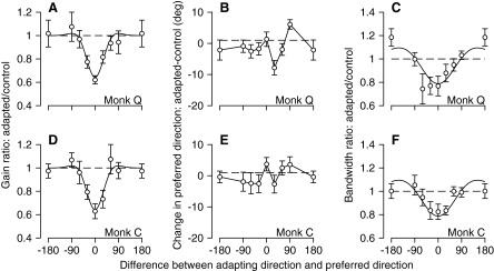
Effect of adaptation with motion in different directions on the average direction tuning parameters of the full MT sample. In all graphs, the change in one parameter of the direction tuning curve is plotted as a function of the difference between the directions of the adapting motion and the preferred direction of the neuron under study. A and D: amplitude of the adapted tuning curve divided by that of the control tuning curve amplitude. B and E: difference in preferred direction of tuning curve before and after adaptation. C and F: bandwidth of the adapted tuning curve divided by that of the control tuning curve. Top and bottom rows show data from monkeys Q and C. Error bars show SEs. The smooth curves in A, C, D, and F show the result of fitting a difference of Gaussians function to the averages across both monkeys. In B and E, points in quadrants I and III indicate direction tuning curves that were repelled from the adapting direction.

Statistical analysis did not reveal any significant differences in the effects of adaptation between the sample recordings in monkeys Q and C. First, an unpaired t-test on the samples for individual combinations of adapting and probe stimuli did not reveal more than a handful of conditions that were significantly different between the two monkeys (P < 0.05). Second, a resampling analysis from the pooled database implied that the individual samples from the two monkeys could be drawn with P > 0.05 from the pooled database. The similarity of the neural recordings from the two animals is emphasized in Fig. 4, A, C, D, and F, where there is good agreement between the data from the individual monkeys and curves obtained by fitting a difference of Gaussians function to the averages of the adaptation effects across the two monkeys.

The reduction in tuning curve amplitude and bandwidth for adapting stimuli in the preferred direction is consistent with the data from Petersen et al. (1985), van Wezel and Britten (2002), and Kohn and Movshon (2004). For adapting directions on the flank of the normal tuning curve, however, the absence of large changes in the preferred direction of the adapted tuning curves is different from the data obtained by Kohn and Movshon (2004) using sine-wave gratings, but consistent with their anecdotal comment about the adapting effects of random-dot textures.

Effect of adapting speed on direction and speed tuning

Adaptation at different speeds had an effect on the speed-tuning curves that mimicked, in most ways, the effect of directional adaptation on direction-tuning curves. Figure 5 illustrates the effect of adaptation at the preferred direction and five different speeds on the speed-tuning curve of an example neuron. The primary effect of speed adaptation was to decrease the amplitude of the speed-tuning curve, in a way that depended on the relationship between the adapting and probe speeds. The decrease in tuning curve amplitude was largest when the adapting speed was the same as the neuron's preferred speed, but also was large when the adapting speed was 50 or 200% of the preferred speed. Effects on tuning bandwidth and preferred speed are also present in the example neuron, but are seen best in the summaries of the population effects.

FIG. 5.

Effect of different speeds of adapting motion on the speed-tuning curve of a representative MT neuron. Each graph plots the average response of the MT neuron as a function of the speed of the testing motion on a logarithmic scale. Open and filled symbols denote data obtained before and after adaptation. The adapting speeds were 25, 50, 100, 200, and 400% of the preferred speed of the neuron under study, indicated by the numbers in the top left corner of each of the 5 graphs.

Across our sample of 47 MT neurons (Fig. 6), speed adaptation affected all three parameters of speed-tuning curves: amplitude, preferred speed, and bandwidth. The average amplitude of the tuning curves decreased by amounts that depended on the ratio of adapting and preferred speed (Fig. 6A), with a maximum decrease to 62% of preadaptation amplitudes when adapting and preferred speed were equal; this agrees well with the decrease to 63% of preadaptation amplitudes in the neurons used to study the effect of adapting direction on direction tuning. Speed adaptation also had a pronounced effect on preferred speed that, on average, repelled the speed-tuning curve away from the adapting speed. It caused a slight increase in preferred speed when the adapting speed was 25% of the preferred speed, no effect when the adapting speed was 50% of the preferred speed, and then a progressively more substantial decrease in preferred speed as the adapting speed increased. When adapting speed was twice the preadaptation preferred speed, the adapted preferred speed was reduced to just over half of control. The effects on tuning bandwidth were smaller, but resulted in narrower bandwidths on average for adapting speeds equal to or half of the preferred speed and slightly wider bandwidths for an adapting speed twice the preadaptation preferred speed. These effects combined so that our data reproduced the effects plotted in Fig. 5 of Krekelberg et al. (2006), confirming their finding that the amount of adaptation, expressed as a percentage of control responses, was greater when the probe speed was different from, rather than the same as, the adapting speed. The good agreement between our data and those of Krekelberg et al. (2006) gives us confidence in the reliability of our speed adaptation results, even though they were obtained on a single monkey.

FIG. 6.

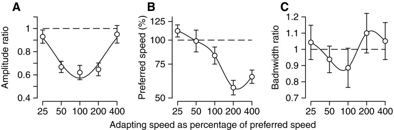
Summary of the effect of adaptation on the parameters of the speed-tuning curves of MT neurons. Each graph plots the average change in one tuning curve parameter across the full sample as a function of the ratio of the adapting speed to the preferred speed, expressed as a percentage on a logarithmic scale. A: response amplitude after adaptation divided by that before adaptation. B: preferred speed after adaptation expressed as a percentage of that before adaptation. C: bandwidth of the speed-tuning curves after adaptation divided by that before adaptation. Error bars show SEs. The smooth curves show the result of fitting a difference of Gaussians function (A) or a cubic spline function (B, C) to the data.

To obtain a complete understanding of adaptation, we also studied the interaction between speed and direction adaptation, by testing the effect of different adapting speeds on directional-tuning curves and of different adapting directions on speed-tuning curves. For these tests, we used either adapting motion in the preferred direction at 50, 100, and 200% of preferred speed or adapting motion at the preferred speed in the preferred direction or ±30° relative to the preferred direction. We did not find large interactions between speed and direction adaptation. For example, the amplitude of the direction-tuning curve decreased, respectively, by 29.9, 28.4, and 25.6% when the adapting speed was 50, 100, of 200% of preferred speed, following the similar effects of the same adapting speeds on speed-tuning curves (Fig. 6A). The amplitude of the speed-tuning function decreased, respectively, by 27.8, 31.8, and 13.2% when the adapting direction was preferred direction −30°, preferred direction, or preferred direction +30°, again in reasonable agreement with the effects of the same adapting directions on direction-tuning curves (Fig. 4, A and D). Therefore we have modeled the interaction between speed and direction of adaptation as a separable function in Eq. 1.

Possible effects of experimental design details on neural expression of adaptation

There are subtle differences between the sequence of adapting and probe stimuli in our experimental design for neural and behavioral measures of adaptation. For behavioral analysis, we used a single long adapting interval followed by a 100- to 300-ms blank period when no stimulus was present, before the fixation point was extinguished and a tracking target appeared. For neural analysis, we used a long adapting interval followed by multiple iterations of the sequence of a 100-ms probe stimulus and 1.5 s of “top-up” adaptation. Figure 7 addresses two key controls showing that: 1) the extent of adaptation was the same in the transient and sustained responses of MT neurons and 2) the blank interval before stimulus presentation in the behavioral experiments did not have large, systematic effects on the properties of neural adaptation (compare top and bottom row of graphs). We also performed behavioral experiments to verify that the iteration of probes and top-ups in the neural experiments did not weaken behavioral adaptation (data not shown).

FIG. 7.

Comparison of direction adaptation of transient and sustained responses for a small sample of MT neurons. Each graph plots the effect of adaptation on a given parameter of the direction tuning curve with the effects on the sustained and transient responses plotted on the y-axis and x-axis. All probe stimuli were 200 ms long and each response was divided into two 100-ms intervals that were used to measure the transient and sustained responses. Top and bottom rows show adaptation with a 100- or 300-ms blank interposed between the adapting and testing stimulus. A: and D: both axes plot the amplitude of the adapted tuning curve divided by that of the control tuning curve. B and E: both axes plot the bandwidth of the adapted tuning curve divided by that of the control tuning curve. C and F: both axes plot the preferred direction of the adapted tuning curve minus that of the control tuning curve.

Behavioral adaptation of pursuit initiation as a function of the speed and direction of adapting and probe stimuli

The second step in our study was to ask whether the neural adaptations observed in MT neurons could be responsible for the behavioral adaptation of pursuit documented previously by Gardner et al. (2004). To provide behavioral adaptations for comparison with decoded neural population responses, we repeated and extended the experiments of Gardner et al. (2004) using an approach outlined in methods. Figure 8, A and D confirms that adaptation with motion at a single speed and direction causes the direction of pursuit to be repelled from the adapting direction when the probe stimuli moved in a range of different directions.

FIG. 8.

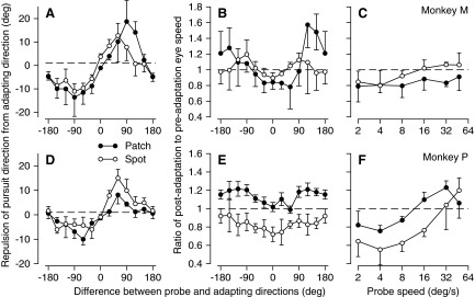
Behavioral adaptations of pursuit direction and speed revealed by probe targets with different forms. A and D: effect of adaptation with motion at 0° on the direction of pursuit for probe motion in different directions. B and E: effect of adaptation with motion at 0° on the speed of pursuit for probe motion in different directions. C and F: effect of adaptation with motion at 16°/s on the speed of pursuit for probe motion at different speeds. Filled and open symbols show results for probe targets consisting of patches of dots or single spots. Horizontal dashed lines show preadaptation values. Top and bottom rows of graphs show data from monkeys M and P.

We also extended the prior work with the observation that adaptation with stimulus motion in a given direction has consistent effects on the speed of the initial pursuit response (Fig. 8, B and E). These curves showed a U-shaped dependence of postadaptation pursuit speed on the difference between the adapting and probe direction, albeit with offsets and amplitudes that varied across monkeys and target forms. When normalized to the speed of pursuit in preadaptation probe trials, the postadaptation speed was smallest when the probe and adapting directions were similar and increased as the probe direction moved further from the adapting direction. In most monkeys, the postadaptation eye speed was smaller than the preadaptation eye speed for probe target motion in the adapting direction; the only exception consisted of the data for monkey P using patches as probe targets (Fig. 8E, filled symbols). Finally, we provide additional data confirming (see Gardner et al. 2004) a consistent relationship between the amount of adaptation of pursuit speed and the speed of probe target motion when adaptation at 16°/s is probed with targets that move at different speeds (Fig. 8, C and F). Postadaptation eye velocity, again normalized for preadaptation values, generally increased as a function of probe speed. As expected, given the normal accuracy of postsaccadic pursuit (Lisberger 1998), preadaptation eye speeds typically were close to target speeds. The only exception was monkey Q who showed very weak postsaccadic eye velocity for the faster target motions.

Both monkeys illustrated in Fig. 8 show the same general trends for all three measures of adaptation of pursuit eye movements, but there are obvious quantitative differences between the two monkeys. In addition, within each monkey, there are differences in the adaptation revealed when probing with spot versus patch targets. However, the two monkeys illustrated in Fig. 8 do not reveal any consistent effects of stimulus form. Adaptation is somewhat larger when probing with spot targets in monkey P, but much larger when probing with patch targets in monkey M. Because the behavioral adaptation curves in Fig. 8 were repeatable across days for a given monkey and probe stimulus, we think that the small differences are real, even if they are not related to the form of the stimulus. In contrast, we showed earlier in the study that the adaptation of MT neurons was statistically identical in the two monkeys used for recordings. Therefore one challenge is to understand how differences in the behavioral adaptation among subjects can be understood in light of the likelihood of similar adaptations of the neural population response. We tackle this issue in the next sections.

Vector-averaging models of population decoding

We think of the population response in MT as a representation of the direction and speed of visual motion and of population decoding as a way of estimating the direction and speed of the original stimulus from the population response. Because we have analyzed the pursuit eye movement that is the direct result of visual motion inputs, we take the estimates provided by a decoding computation as an index of the direction and speed commands for pursuit. Thus by evaluating how adaptation alters the decoded estimates of target direction and speed, we can predict how it should affect the adaptation recorded in the initiation of pursuit eye movements.

To assess the relationship between neural adaptation in MT and behavioral adaptation of pursuit direction and speed, we made an MT population model that comprised 4,608 model units, uniformly distributed in direction (72 preferred directions) and log₂ of speed (64 preferred speeds). Each model neuron's preadaptation and postadaptation firings were calculated by plugging the relevant parameters into Eq. 1. For postadaptation responses, each unit's values of preferred direction/speed, bandwidth, and response gain were taken from the smooth curves used to fit the population averages in Figs. 4 and 6. The polar contour plot in Fig. 9 illustrates the response of the model MT population to a probe stimulus moving at 16°/s in a direction that is rotated 30° clockwise relative to rightward. Compared with control responses (red contour lines), adaptation with motion at 16°/s to the right caused the peak of the population response (blue contour lines) to be repelled away from the adapting direction, toward neurons that preferred more downward directions. At the same time there was relatively little change, or perhaps only a slight decrease, in the preferred speed of the model neurons with the largest responses.

FIG. 9.

Response surface on a polar plot showing the effect of adaptation on the responses of a population of model MT neurons with a wide range of preferred directions and preferred speeds. For this example, the adapting direction was rightward and the testing motion was rotated 30° clockwise from rightward so that it included some downward motion. The red and blue contour lines show the amplitude of the population responses before and after adaptation for model neurons as a function of their preferred direction and speed. Thus each pixel on the contour lines represents the end of a vector whose length is equal to the preferred speed of the model neuron at that pixel and whose angle represents the preferred direction of the model neuron at that pixel. Thicker contour lines indicate larger response values. The model population was based on data from monkey C.

The decoding computation known as “vector averaging” provides a way to estimate the preferred speed and direction of the most active neurons in the population or, more accurately, to estimate the center of mass of the population. We call this the “separate” decoding model, described as

(2)

(3)

where θ and S are the direction and speed of target motion, respectively, and θ′ and S′ are the estimates obtained by decoding the population response in MT. In Eqs. 2 and 3, MT_i(θ, S) is the response of the ith model MT unit as a function of θ and S and PS_i and Pθ_i are, respectively, its preferred speed and direction. Here and below, ɛ is a scalar that makes each decoding computation resistant to noise and low values of population response (Churchland and Lisberger 2001; Weiss et al. 2002). The value of ɛ was set to 0.05 and did not have any impact on the predictions of the model for the large-amplitude model population responses in our simulations.

Although vector averaging is intuitively pleasing, it has two practical disadvantages. First, it provides outputs in the form of a vector that preserves the retinal coordinate frame of the visual motion representation in MT; the vector eventually must be transformed to the motor coordinates defined by the pulling directions of the extraocular muscles. Second, an opponent motion signal was required to account for prior data (e.g., Churchland and Lisberger 2001) and some of the data presented here (see the following text). However, for a two-dimensional population code, it is not clear how to implement an opponent decoding computation for target speed based on vector averaging without first knowing the axis of target motion.

To resolve the drawbacks of pure vector averaging as represented by Eqs. 2 and 3, we also explored the predictions of a decoding model that uses vector averaging from different subsets of MT neurons to decode a command for desired smooth eye velocity in motor, rather than sensory coordinates. The “joint” decoding model is described as

(4)

(5)

(6)

where and are the decoded commands for the horizontal and vertical components of eye velocity, MT_i is the firing, and PS_i and Pθ_i are the preferred speed and direction of the ith MT neuron. The model weights each neuron's contribution according to the sine or cosine of its preferred direction; the positive and negative lobes of the sine/cosine functions provide the weights needed to create an opponent motion signal. The model converts the sensory representation of visual motion from retinal coordinates to an approximation of the pulling directions of extraocular muscles and we calculate the speed and direction of eye motion by combining those two vectors.

Figure 10 compares the performance of the “separate” and “joint” vector-averaging decoding models for the three manifestations of behavioral adaptation illustrated in Fig. 8. Here, the parameters of the model neurons and the effects of motion adaptation on those parameters were based on population averages across our sample of MT neurons. Both the joint and separate decoding models made the same predictions for the effect of adaptation on the direction of pursuit (Fig. 10, A and D). Both predicted that the direction of pursuit would be repelled from the adapting direction and, for both models, the repulsion resulted mainly from adaptation of the bandwidth of direction-tuning curves. In disagreement with the prediction of Gardner et al. (2004), adaptation of the amplitude of tuning curves contributed only slightly to direction repulsion. The two decoding models also made similar predictions for the effect of probe speed on the adaptation of initial pursuit speed (Fig. 10, C and F). However, the two models differed in their predictions for the adaptation of initial pursuit speed as a function of the difference between the adapting and probe direction. The joint decoding model predicted a U-shaped function (Fig. 10B) like that seen in our data, whereas the separate decoding model predicted an inverted U-shaped function (Fig. 10E) that disagreed with our data. We think that the shape of the speed adaptation function in Fig. 10, B and E is related to the presence and absence of an opponent motion signal in the decoding computation. Unfortunately, we could not demonstrate our intuition rigorously because an opponent motion signal cannot be defined when decoding speed using a separate vector-averaging model for a population response that covers the full range of both preferred speeds and preferred directions.

FIG. 10.

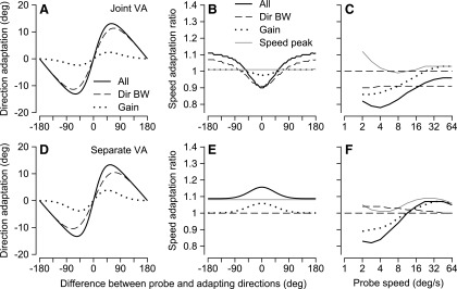
Predictions of joint (A–C) and separate (D–F) vector averaging decoding computations for direction and speed adaptation of pursuit, given a model population response based on the mean of our sample. A and D: adaptation of pursuit direction as a function of the difference between probe and adapting directions. B and E: adaptation of pursuit speed as a function of the difference between probe and adapting directions. C and F: adaptation of pursuit speed as a function of probe speed when adapting speed was 16°/s. Different line types indicate the contributions to behavioral adaptation from adapting different individual parameters of the MT population response. The key in A also applies to D. They key in B applies to C, E, and F as well. In C and F, the horizontal dashed line is at one on the y-axis.

Population decoding to account for behavioral adaptation in pursuit

If only a subset of MT neurons contributes to pursuit and the relevant subset varied across monkeys, then different amounts of behavioral adaptation might occur in different monkeys even with the same amount of adaptation in the neural population response. To test the plausibility of this idea, we extended the predictions of Fig. 10, A–C, which were based on the average responses of our sample of neurons for the joint decoding model. We systematically evaluated the model's predictions for behavioral adaptation under different assumptions about the properties of the neurons that contributed to the decoding computation. Figure 11 evaluates the effect of varying the amount of adaptation of response amplitude or gain (Fig. 11, A–C), the amount of adaptation of direction bandwidth (Fig. 11, D–F), the width of the preadaptation direction tuning (Fig. 11, G–I) and speed-tuning (Fig. 11, J–L) curves, and the baseline firing (Fig. 11, M–O). For the first four rows of graphs, varying the value of the different parameters from 0.5- to twofold their average values had different effects on adaptation. Varying the amount of adaptation of response gain (Fig. 11, A–C) primarily affected the expression of adaptation at different probe speeds (Fig. 11C). The amount of direction repulsion was affected mostly by the amount of direction bandwidth adaptation (Fig. 11D) and the baseline direction bandwidths (Fig. 11G) of the model MT neurons that contributed to the decoding computations. The adaptations of pursuit speed as a function of probe direction and speed were affected by most parameters, but in different ways by each parameter. In the last row of graphs in Fig. 11, varying the baseline firing as a proportion of the maximal responses from 0 to 0.2 affected the amount of speed adaptation (Fig. 11, N and O), without any impact on direction adaptation (Fig. 11M). We have not included graphs to show the effects of varying the amount of adaptation of the preferred speed because there was none. We conclude that selecting from different subsets of MT neurons has the potential to lead to different amounts of behavioral adaptation in different monkeys.

FIG. 11.

Effect of selecting outputs from different subsets of MT neurons on the predictions of the joint vector averaging decoding model for behavioral adaptation. From left to right, the columns of graphs show adaptation of pursuit direction as a function of the difference between probe and adapting directions, adaptation of pursuit speed as a function of the difference between probe and adapting conditions, and adaptation of pursuit speed as a function of probe speed when adapting speed was 16°/s. The 5 rows show the effect of varying 5 different features of the population responses, according to the labels at the right of each row. Different colored traces show predicted adaptation for different sets of parameters, according to the keys to the right of A and M. Key in A applies to A–L and each entry indicates the multiplication factor applied to the mean for the parameter varied in a given plot; key in M applies to M–O and each entry indicates the value of the baseline firing as a fraction of the maximum response of each model neuron.

Figure 12 illustrates that it was possible to select physiologically reasonable parameters for the population response and its adaptation and account for each of the different adaptations in each monkey we tested, where each row of graphs shows three manifestations of adaptation for a given monkey and probe target form. For four of the six sets of monkey/target conditions, the model (continuous curves) fitted the data (open symbols) quite well and fell within the bounds defined by 1SD of the adaptation data across experimental days (error bars). For the remaining two sets of behavioral adaptations (Fig. 12, G–I and P–R), the model predictions were poor for the effect of probe speed on speed adaptation (Fig. 12, I and R), but were excellent for the other data. We allowed only four parameters of the population response to vary in choosing the best fit for each set of behavioral adaptations: the amount of adaptation in response amplitude, the amount of direction bandwidth adaptation, and the direction and speed bandwidths of the unadapted model neurons. Table 1 presents the values that provided the best fits for each of the six sets of adaptations.

FIG. 12.

Comparison of the behavioral effects of direction adaptation on pursuit eye movements with the predictions obtained by decoding the model MT population response. From left to right, the columns of graphs show adaptation of pursuit direction as a function of the difference between probe and adapting directions, adaptation of pursuit speed as a function of the difference between probe and adapting conditions, and adaptation of pursuit speed as a function of probe speed when adapting speed was 16°/s. Each row shows analysis for one combination of monkey and target form, indicated by text at the right of the graphs in the left column. In each graph, the connected symbols show the data from behavioral adaptations and the curves show the predictions of the model that reproduced the data most accurately.

TABLE 1.

Values of parameters in the model MT population that provided the best fit to the behavioral adaptation for different combinations of monkeys/targets

Monkey and Target	Δ Response Amplitude	Δ Direction Bandwidth	Direction Bandwidth	Speed Tuning SD
C, spot	0.5	0.8	70	1.5
Q, spot	2.0	0.8	20	1.5
P, spot	0.5	0.5	40	0.4
P, patch	2.0	0.5	50	2.0
M, spot	2.0	0.7	50	2.0
M, patch	1.0	0.8	80	2.0

For the “Δ Response Amplitude” and “Δ Direction Bandwidth” the numbers indicate the amount of adaptation as a multiple of the mean adaptation for the entire sample of MT neurons. For the “Direction Bandwidth” the numbers indicate the half-width of the model tuning curves. For the “Speed Tuning SD” the numbers indicate the SD of the speed tuning curves in units of log₂ (speed).

DISCUSSION

Motion adaptation has been documented many times in perception, motor control, and the responses of central neurons. However, the link from neural adaptation to perceptual or motor adaptation is understood poorly (Kohn 2007). Advances in understanding the link from adapted neural to behavioral responses would provide insight into normal sensorimotor transformations, which themselves are probably not modified by adaptation. Establishing the link from adapted neural to behavioral responses requires documentation of how adaptation alters the responses of a population of neurons along with quantitative measures of behavior for a wide range of stimuli. A number of prior reports have provided pieces of the requisite neural or behavioral data for adaptation of responses to visual motion (e.g., Gardner et al. 2004; Kohn and Movshon 2004; Krekelberg et al. 2006). Our study goes further by measuring a larger set of neural and behavioral adaptations in a single species for a full set of motion stimuli, constructing models of realistic population responses before and after adaptation, and showing that a single decoding computation can link neural and behavioral adaptation quantitatively.

We have shown that we can account for the differences in the magnitude of behavioral adaptation among monkeys by assuming that pursuit in different monkeys is driven by subsets of MT neurons with different response parameters. The success of our decoding model shows that behavioral adaptation is represented fully in the population response in MT, implying that a single, sensory locus of adaptation is plausible. It also gives us some hope that the decoding equations may map onto neural mechanisms, but the most important conclusion is that a simple decoding model can account for the direction and speed adaptation in different monkeys, even under the assumption (supported by our neural data) that the adaptation of the population response in MT does not differ among monkeys. However, the success of our model does not show directly either that the decoding computation we used is the same as the one used in the brain or that pursuit draws from a subset of MT neurons that could vary across monkeys. We also cannot deal fully with the difference in behavioral adaptation for different stimulus forms within an individual monkey. Thus it is not clear whether we can explain the different adaptations for spot and patch probe targets in terms of subtly different response properties in MT for moving spots versus moving dot textures. This will have to be the topic of future MT recordings.

We have adopted the vector-averaging framework because our prior work emphasized the virtues and successes of vector averaging as a decoding computation (e.g., Churchland and Lisberger 2001; Priebe and Lisberger 2004). We have retained the use of an opponent motion signal because it was needed to account for the transformation of the MT population response into pursuit eye movements for apparent motion stimuli (Churchland and Lisberger 2001) and it also allowed us to simulate the adaptation of pursuit speed as a function of probe target direction. At the same time, we have moved toward a model that copes gracefully with the creation of an opponent motion signal and with the challenge of programming simultaneously the direction and speed of pursuit eye movements by decoding horizontal and vertical speed components separately. The use of horizontal and vertical decoding functions for speed mimics the fact that the neural commands for smooth eye movement must eventually be broken down into muscle coordinates, which are approximately horizontal versus vertical. We used sine and cosine weighting functions to select the MT neurons that would contribute to decoding along each axis, mainly because this minimized the number of free parameters in the model. However, it would be possible to use Gaussian weighting functions for neurons that contribute to the vertical and horizontal components of pursuit, allowing changes in the width of the Gaussians to serve as an additional parameter that might allow the decoding model to account for other kinds of data in the future. It also would have been possible to use maximum-likelihood computations (after Jazayeri and Movshon 2006) along the horizontal and vertical axes, as long as pursuit received inputs selectively from subsets of MT neurons with different response properties.

Two issues remain. One is whether we can explain why our computational analysis reproduced directional adaptation better than speed adaptation. We cannot, although we do think that the excellent predictions of pursuit direction and the broad qualitative agreement between the predicted and actual adaptations of pursuit speed endorse our computational analysis as a good start. The other issue is whether other mechanisms could account for the different amounts of directional adaptation in different monkeys. As we will enumerate here, most other explanations for differences in behavioral adaptation are inconsistent with available data. 1) Our data show that adaptation caused very similar alternations of the neural population responses in MT of the two monkeys we studied, implying the differential behavioral adaptation cannot be attributed to different neural adaptations within MT. 2) We found similar amounts of adaptation across neurons with broad and narrow spike waveforms, arguing that projection neurons and interneurons adapt similarly. Therefore a failure to thoroughly sample the neurons that contribute to pursuit behavior probably cannot be invoked to explain the different amounts of behavioral adaptation in different monkeys. 3) The absence of consistent effects of target form on behavioral adaptation argues that differences in target form cannot explain the differences in behavioral adaptation across monkeys. 4) Correlations in the responses of different MT neurons do not play an important role in motion adaptation; spike count correlations are quite small (Bair et al. 2001) and simulations of the effects of neuron–neuron correlations indicate that they affect the magnitude of trial-by-trial variation, but not the mean responses that were measured here (X. Huang and S. G. Lisberger, unpublished observations).

The novelty of our study resides in our finding that we can understand pursuit adaptation in terms of the adaptation of neural population responses and in our quantitative evaluation of the relationship between behavioral and neural adaptation. Our neural data are more complete, but in good agreement with, those in prior studies insofar as stimulus conditions overlapped. We agree with Petersen et al. (1985) and van Wezel and Britten (2002) that an adapting stimulus in the preferred direction of the neuron under study causes a reduction in the amplitude of the direction-tuning curve, whereas adaptation in the opposite direction causes a small enhancement of the amplitude of the tuning curve. We agree with Krekelberg et al. (2006) that adaptation reduces the amplitude and the bandwidth of speed tuning in a way that leads to a larger percentage change on the flanks versus the peaks of the speed-tuning curves. Our results are different from those of Kohn and Movshon (2004), but so were our stimuli. They used moving sine-wave gratings to study the responses of MT neurons and found that adaptation narrowed the bandwidth of direction-tuning curves (our data agree) and attracted the tuning curve toward the adapting direction. We used dot textures as stimuli and found that adaptation had little effect on the preferred direction of MT neurons and repelled speed-tuning curves from the adapting speed. Kohn and Movshon (2004) note, however, that unpublished results using dot textures agreed with our data, implying that the differences between our data and theirs are probably due to differences in stimulus form. It is noteworthy that the different effects of adaptation on the population responses for dot textures (our study) and sine-wave gratings (Kohn and Movshon 2004), once processed by a decoding computation, yield similar predictions for direction adaptation of pursuit.

Thus our study demonstrates that motion adaptation in the pursuit of macaque monkeys can be explained on the basis of the neural population response derived from MT recordings made in awake subjects of the same species. In contrast to our study, which provides full data sets for both behavioral and neural adaptation of both direction and speed, prior reports have provided only pieces of the story. Kohn and Movshon (2004) studied only direction adaptation in anesthetized monkeys and compared their results to adaptation of human direction perception. Gardner et al. (2004) studied direction adaptation in pursuit of behaving monkeys, but provided an explanation based on conjecture about the concomitant neural adaptations. Krekelberg et al. (2006) addressed a question somewhat different from ours. They focused on the predictive value of single neurons and on a population decoding computation that was useful for discrimination of higher versus lower speeds, but not for identification of the speed and direction of target motion required for control of smooth-pursuit eye movements.

It seems inevitable that the decoding computations used in the brain to convert neural population responses into predictions of behavioral adaptation will differ, at least in detail, from the representations provided by equations for vector averaging. Thus it is certain that the decoding computations we have used to predict pursuit adaptation are wrong in the sense that they are not exactly the ones used in the brain. However, our prior work on the relationship between neural population responses and pursuit establishes that vector averaging provides an excellent surrogate for the decoding computations used by the brain (Churchland and Lisberger 2001; Priebe and Lisberger 2004). Further, vector averaging provides an almost unbiased way to estimate the amount of adaptation in the population response (Salinas and Abbott 1994). The next step toward improving the quantitative match between predicted and actual behavioral adaptations may be to better understand the neural implementation of the equations we have used as decoding functions. This step may be particularly important for understanding decoding for motion perception, which could work differently because it need not provide an output in the motor coordinates of the extraocular muscles.

GRANTS

This work was supported by the Howard Hughes Medical Institute and by National Eye Institute Grant EY-03878.

REFERENCES

- Albright 1984.Albright TD Direction and orientation selectivity of neurons in visual area MT of the macaque. J Neurophysiol 152: 1106–1130, 1984. [DOI] [PubMed] [Google Scholar]
- Bair et al. 2001.Bair W, Zohary E, Newsome WT. Correlated firing in macaque visual area MT: time scales and relationship to behavior. J Neurosci 21: 1676–1697, 2001. [DOI] [PMC free article] [PubMed] [Google Scholar]
- Born et al. 2000.Born RT, Groh JM, Zhao R, Lukasewycz SJ. Segregation of object and background motion in visual area MT: effects of microstimulation on eye movements. Neuron 26: 725–734, 2000. [DOI] [PubMed] [Google Scholar]
- Churchland et al. 2007.Churchland AK, Huang X, Lisberger SG. Responses of neurons in the medial superior temporal visual area to apparent motion stimuli in macaque monkeys. J Neurophysiol 97: 272–282, 2007. [DOI] [PMC free article] [PubMed] [Google Scholar]
- Churchland and Lisberger 2001.Churchland MM, Lisberger SG. Shifts in the population response in the middle temporal visual area parallel perceptual and motor illusions produced by apparent motion. J Neurosci 21: 9387–9402, 2001. [DOI] [PMC free article] [PubMed] [Google Scholar]
- Dubner and Zeki 1971.Dubner R, Zeki SM. Response properties and receptive fields of cells in an anatomically defined region of the superior temporal sulcus in the monkey. Brain Res 35: 528–532, 1971. [DOI] [PubMed] [Google Scholar]
- Gardner et al. 2004.Gardner JL, Tokiyama SN, Lisberger SG. A population decoding framework for motion aftereffects on smooth pursuit eye movements. J Neurosci 24: 9035–9048, 2004. [DOI] [PMC free article] [PubMed] [Google Scholar]
- Jazayeri and Movshon 2006.Jazayeri M, Movshon JA. Optimal representation of sensory information by neural populations. Nat Neurosci 9: 690–696, 2006. [DOI] [PubMed] [Google Scholar]
- Kohn 2007.Kohn A Visual adaptation: physiology, mechanisms, and functional benefits. J Neurophysiol 97: 3155–3164, 2007. [DOI] [PubMed] [Google Scholar]
- Kohn and Movshon 2003.Kohn A, Movshon JA. Neuronal adaptation to visual motion in area MT of the macaque. Neuron 39: 681–691, 2003. [DOI] [PubMed] [Google Scholar]
- Kohn and Movshon 2004.Kohn A, Movshon JA. Adaptation changes the direction tuning of macaque MT neurons. Nat Neurosci 7: 764–772, 2004. [DOI] [PubMed] [Google Scholar]
- Krekelberg et al. 2006.Krekelberg B, van Wezel RJ, Albright TD. Adaptation in macaque MT reduces perceived speed and improves speed discrimination. J Neurophysiol 95: 255–270, 2006. [DOI] [PubMed] [Google Scholar]
- Levinson and Sekuler 1976.Levinson E, Sekuler R. Adaptation alters perceived direction of motion. Vision Res 16: 779–781, 1976. [DOI] [PubMed] [Google Scholar]
- Lisberger 1998.Lisberger SG Postsaccadic enhancement of initiation of smooth pursuit eye movements in monkeys. J Neurophysiol 79: 1918–1930, 1998. [DOI] [PubMed] [Google Scholar]
- Lisberger and Movshon 1999.Lisberger SG, Movshon JA. Visual motion analysis for pursuit eye movements in area MT of macaque monkeys. J Neurosci 19: 2224–2246, 1999. [DOI] [PMC free article] [PubMed] [Google Scholar]
- Maunsell and Van Essen 1983.Maunsell JH, Van Essen DC. Functional properties of neurons in middle temporal visual area of the macaque monkey. I. Selectivity for stimulus direction, speed, and orientation. J Neurophysiol 49: 1127–1147, 1983. [DOI] [PubMed] [Google Scholar]
- Mitchell et al. 2007.Mitchell JF, Sundberg KA, Reynolds JH. Differential attention-dependent response modulation across cell classes in macaque visual area V4. Neuron 55: 131–141, 2007. [DOI] [PubMed] [Google Scholar]
- Newsome et al. 1989.Newsome WT, Britten KH, Movshon JA. Neuronal correlates of a perceptual decision. Nature 341: 52–54, 1989. [DOI] [PubMed] [Google Scholar]
- Newsome et al. 1985.Newsome WT, Wurtz RH, Dürsteler MR, Mikami A. Deficits in visual motion processing following ibotenic acid lesions of the middle temporal visual area of the macaque monkey. J Neurosci 5: 825–840, 1985. [DOI] [PMC free article] [PubMed] [Google Scholar]
- Osborne et al. 2007.Osborne LC, Hohl SS, Bialek W, Lisberger SG. Time course of precision in smooth pursuit eye movements. J Neurosci 27: 2987–2998, 2007. [DOI] [PMC free article] [PubMed] [Google Scholar]
- Petersen et al. 1985.Petersen SE, Baker JF, Allman JM. Direction specific adaptation in area MT of the owl monkey. Brain Res 346: 146–150, 1985. [DOI] [PubMed] [Google Scholar]
- Priebe and Lisberger 2004.Priebe NJ, Lisberger SG. Estimating target speed from the population response in visual area MT. J Neurosci 24: 1907–1916, 2004. [DOI] [PMC free article] [PubMed] [Google Scholar]
- Ramachandran and Lisberger 2005.Ramachandran R, Lisberger SG. Normal performance and expression of learning in the vestibulo-ocular reflex (VOR) at high frequencies. J Neurophysiol 93: 2028–2038, 2005. [DOI] [PMC free article] [PubMed] [Google Scholar]
- Salinas and Abbott 1994.Salinas E, Abbott LF. Vector reconstruction from firing rates. J Comput Neurosci 1: 89–107, 1994. [DOI] [PubMed] [Google Scholar]
- Salzman et al. 1992.Salzman CD, Murasugi CM, Britten KH, Newsome WT. Microstimulation in visual area MT: effects on direction discrimination performance. J Neurosci 12: 2331–2355, 1992. [DOI] [PMC free article] [PubMed] [Google Scholar]
- Schrater and Simoncelli 1998.Schrater PR, Simoncelli EP. Local velocity representation: evidence from motion adaptation. Vision Res 38: 3899–3912, 1998. [DOI] [PubMed] [Google Scholar]
- Stone and Lisberger 1990.Stone LS, Lisberger SG. Visually driven output from the primate flocculus. I. Simple-spike responses to the visual inputs that initiate pursuit eye movements. J Neurophysiol 63: 1241–1261, 1990. [DOI] [PubMed] [Google Scholar]
- Tanaka and Lisberger 2001.Tanaka M, Lisberger SG. Regulation of the gain of visually guided smooth-pursuit eye movements by frontal cortex. Nature 409: 191–194, 2001. [DOI] [PubMed] [Google Scholar]
- Van Wezel and Britten 2002.Van Wezel RJA, Britten KH. Motion adaptation in area MT. J Neurophysiol 88: 3469–3476, 2002. [DOI] [PubMed] [Google Scholar]
- Weiss et al. 2002.Weiss Y, Simoncelli EP, Adelson EH. Motion illusions as optimal percepts. Nat Neurosci 5: 598–604, 2002. [DOI] [PubMed] [Google Scholar]