Predicting protein folding cores by empirical potential functions

Abstract

Theoretical and in vitro experiments suggest that protein folding cores form early in the process of folding, and that proteins may have evolved to optimize both folding speed and native-state stability. In our previous work, we developed a set of empirical potential functions and used them to analyze interaction energies among secondary-structure elements in two β-sandwich proteins. Our work on this group of proteins demonstrated that the predicted folding core also harbors residues that form native-like interactions early in the folding reaction. In the current work, we have tested our empirical potential functions on structurally-different proteins for which the folding cores have been revealed by protein hydrogen-deuterium exchange experiments. Using a set of 29 unrelated proteins, which have been extensively studied in the literature, we demonstrate that the average prediction result from our method is significantly better than predictions based on other computational methods. Our study is an important step towards the ultimate goal of understanding the correlation between folding cores and native structures.

Introduction

Understanding the mechanisms by which proteins fold is one of the grand challenges of molecular biology. Theoretical studies suggest a funnel-like free energy landscape for protein folding, which helps to explain how an extended polypeptide chain consistently folds into its stable native three-dimensional conformation in a speedy fashion [1-4].

Theoretical and in vitro experiments suggest that protein folding nuclei, or cores, form early in the folding process [5-13]. This finding, in turn, supports Hammond’s postulate [14] that thermodynamics and kinetics are closely correlated in proteins and that proteins may have evolved to optimize both folding rate and native-state stability [15]. Our earlier combined experimental-theoretical study on Pseudomonas aeruginosa apo-azurin and another β-sandwich protein demonstrated this correlation, in which the stable folding cores predicted by our energetic method also harbored the key residues involved in the folding-transition [5].

Among the experimental methods to probe the protein folding process, protein hydrogen-deuterium exchange (HX)² helps identify protein regions that are shielded from solvent and thus “protected” from deuterium exchange (i.e., resulting in a slower rate of exchange). Based on HX experiments, the hydrogen-bonded amide protons (NHs) that are most protected from deuterium exchange in the protein native-state are often found in the same protein regions as the NHs protected earliest during the protein folding reaction, as well as those NHs that are most protected in partially-folded intermediate states of the protein [13,16,17]. In contrast, NHs in turns and loops are rarely among the very slowest protons to exchange. Therefore, HX is useful in identifying the slow-exchanging NHs that make up the protein folding core.

Several computational models have been developed that try to connect folding theory with experimental data on protein unfolding/folding kinetics. Examples are graph-theoretical approaches based on effective contact order [18,19], several variants of a motion planning method [20-23], molecular dynamics simulations of unfolding fluctuations around the native-state [24,25], an unfolding approach using a secondary-structure contact network and minimum cuts [26], a simplified lattice-protein model of native-state HX [27], and a method that exploits a correlation between slowest exchanging cores and low conformational entropy [28]. The two most relevant examples of computational models, with respect to this study, are the Floppy Inclusions and Rigid Substructure Topography (FIRST) method [29] and the Gaussian Network Model (GNM) [15,30]. In the FIRST method, inter-atomic covalent and hydrogen bonds and hydrophobic interactions are replaced by rigid bars whose lengths and bond angles are constrained—only bond rotations are allowed. FIRST then identifies the rigid and flexible parts of the all-atomic protein model by selectively breaking hydrogen bonds in order of weakest to strongest. The GNM method coarse-grains a protein into an elastic network of residues, whereby pairs of residues within a cut-off distance are connected by virtual elastic springs, and it predicts the stable folding cores by studying the collective motions of the elastic network. In GNM, slow mode minima imply hinge sites, whereas high frequency mode peaks indicate stable “kinetically hot” residues.

Despite some success with these computational methods, there remains room for improvement. Empirical potential functions have been used previously to study changes in protein stability [31-33]. In our former work [5], we developed an empirically-weighted set of statistical potential functions and used them to analyze interaction energies among secondary-structure elements in two β-sandwich proteins. In the current study, we test the power of our empirical potential functions by applying them to the prediction of protein folding cores as revealed by HX experiments, using a large set of proteins with different structures.

Here, and in earlier studies [13,15], the experimental folding cores are defined as those that make up the folding core elements, which are the secondary-structure elements (SSEs) containing the slowest exchanging residues (those with the greatest protection factors) identified in HX experiments. Using a set of 29 unrelated proteins that were extensively studied in the literature, we show that, on average, our predictions correlate better with the experimentally-identified folding cores than those of two GNM methods and a third method using the FIRST software. We believe that our prediction method may be useful to facilitate a better understanding of the factors that dictate protein folding and native-state stability.

Materials and methods

Choice of experimental data and protein folding core prediction targets

HX experiments are typically subdivided into three types based on their detection purposes and experimental settings [13]: slow exchange core experiments (for NHs most protected in the native-state), pulsed exchange experiments (for NHs first protected during folding), and folding competition experiments (for NHs most protected in partially-folded species). The folding core secondary-structure elements (SSEs) revealed by these three methods are often identical or very similar. Thus, we follow Rader and Bahar [15] in using experimental data from slow exchange core experiments, the most abundant experimental folding core data in the literature, as our prediction targets. In addition, the secondary-structure definitions are based on the Protein Data Bank SHEET and HELIX records.

To train our empirical potential function and then compare our computational predictions with experimental results, we used a set of 29 proteins (listed in Table 1) that were extensively studied in the literature [13,15,34-40].

Table 1.

Proteins used in this study

	Name	Abbrev.	PDB code	# of SSEs
(a) The testing set
1	Apo-myoglobin	apoMb	1mbo	8
2	Barnase	Bnase	1a2p	8
3	Cytochrome c	Cytc	1hrc	5
4	T4 lysozyme	T4lzm	2lzm	14
5	Ribonuclease T1	RnaseT1	9rnt	8
6	α-Lactalbumin	ha-LA	1hml	12
7	Chymotrypsin inhibitor 2	CI2	2ci2	5
8	Ubiquitin	Ubq	1ubi	7
9	Bovine pancreatic trypsin inhibitor	BPTI	5pti	5
10	Interleukin-1β	IL-1b	1i1b	14
11	Hen egg-white lysozyme	HEWL	1hel	10
12	Equine lysozyme	Eqlzm	2eql	10
13	Protein A, B-domain	pAB	1bdd	3
14	Ribonuclease A	RnaseA	1rbx	10
15	Guinea pig α-lactalbumin	gpa-LA	1hfx	9
16	B1 immunoglobulin-binding domain protein G	GB1	1pga	5
17	B1 immunoglobulin-binding domain protein L	LB1	2ptl	5
18	Cardiotoxin analog III	CTX-3	2crt	5
19	Tendamistat	Tnds	2ait	6
20	Single chain antibody fragmenta	scFv	2mcp	23
21	Human acidic fibroblast growth factor-1	hFGF-1	2afg	14
22	Cytochrome c551	pacc551	351c	5
23	Outer surface protein A	ospA	1osp:O	24
24	Ovomucoid third domain	OMTKY3	1iy5	4
25	Chicken src SH3 domain	cSH3	1srm	6
26	CheY	CheY	3chy	10
27	Human carbonic anhydrase I	HCA-1	1hcb	22
(b) The training set
28	Staphylococcal nuclease	Snase	1stn	9
29	Ribonuclease H	RnaseH	2rn2	10

^aFor consistency with previous studies [13,15], we consider only the residues 1-115 in chain L and 1-122 in chain H.

Prediction of folding cores based on an empirical potential function

The computational prediction method using our all-atom empirical potential function is described in detail in our previous work [5]. The stability cores are ranked by the interaction energy between multiple SSEs (groups of two, three or four) using a scoring function:

$$S_{\text{core}}=3.45{\stackrel{‒}{E}}_{\text{Packing}}+5.0{\stackrel{‒}{E}}_{\mathrm{AS}}+1.9{\stackrel{‒}{E}}_{\mathrm{HB}}.$$ (1)

Here, the three terms in the scoring function represent the effects of side-chain packing (Ē_Packing), solvent accessible surface area (Ē_AS), and hydrogen bonding interactions (Ē_HB), respectively. The parameters for these three terms are statistically derived from a non-redundant structure database of 2701 non-homologous soluble proteins [41], and the weight for each term is chosen by fitting to the folding core results of two proteins with the most consistent HX data [13], listed in Table 1b. These two proteins, staphylococcal nuclease [42,43] and ribonuclease H [44,45], both have α-helix and β-sheet SSEs, and they are excluded from the set of 27 proteins used for cross-validation.

For comparison with the experimental HX results by Li and Woodward [13], we define the folding core as the group of SSEs with the lowest interaction energy. The interaction energies are calculated for groups of two, three and four SSEs, and each grouping type is considered a separate but related method for predicting the folding core.

Evaluation of overlap between predictions and experiments

To compare our approach to previous methods and experimental results, we adopted the method for evaluating overlap employed by Rader and Bahar [15]. There are two related measures for the overlap between methods A and B (A and B may be experimental or computational prediction methods):

$$s(A,B)=\frac{o(A,B)}{\frac{N_A\cdot N_B}{N}},$$ (2)

$$z(A,B)=o(A,B)-\frac{N_A\cdot N_B}{N}.$$ (3)

Here, N is the total number of residues in the target protein, N_A and N_B are the numbers of folding core residues revealed by methods A and B, respectively, and o(A, B) is the overlap in the number of residues revealed by methods A and B. These two quantities s(A, B) and z(A, B) measure the extent of difference between the observed overlap, o(A, B), and the expected overlap for random matches, N_A · N_B/N. Thus, s = 1 and z = 0 correspond to random matches and larger values of s and z indicate greater correlation between methods A and B.

Results and discussion

Fig. 1 illustrates the folding cores predicted by HX experiments and the empirical potential function for a few examples within the 27-protein test set. Folding core elements are mapped as dark ribbons on the light gray 3D cartoon backbone of the protein structure. Each column represents one of the four methods (HX experiments; two-, three- and four-SSE interaction groups). Fig. 2 summarizes the comparisons of the four methods for all 27 test proteins using the reduced representation from Rader and Bahar [15]. The x-axis corresponds to the residue index, and the stacked bars represent the experimentally-determined or predicted folding core elements. With the exceptions of ha-LA, CTX-3, and Eqlzm, the predictions yielded by the empirical potential function have substantial overlap with the experimental results. Fig. 3 overlaps experimental phi values with the folding core elements determined by the four methods for 10 of the 27 test proteins.

Fig. 1.

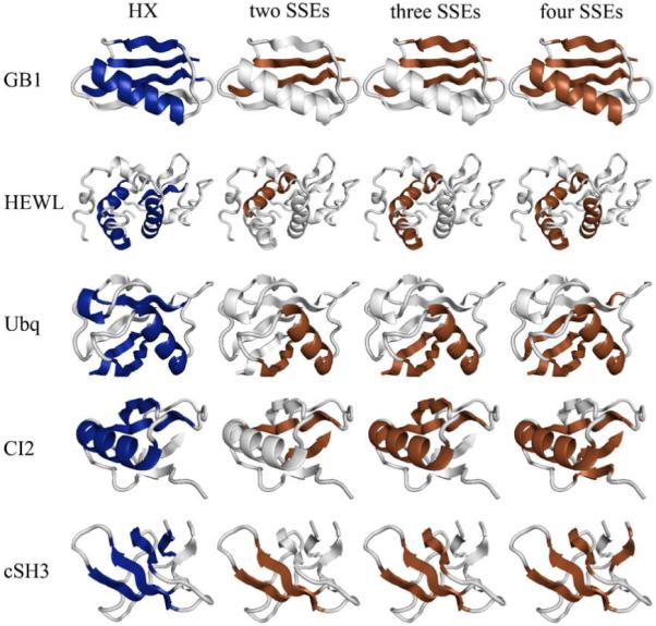
Folding cores predicted by HX experiments and the empirical potential function for a few examples (GB1, HEWL, Ubiquitin, CI-2 and cSH3) within the 27-protein test set. Folding core elements are mapped as dark ribbons on the light gray 3D cartoon backbone of the protein structure. Each column represents one of the four methods (HX experiments; two-, three- and four-SSE interaction groups). The cartoons were generated using PyMOL (DeLano Scientific, LLC).

Fig. 2.

Comparison of folding cores predicted by HX experiments and the empirical potential function (for four-, three- and two-SSE interaction groups) for all 27 test proteins using the reduced representation from Rader and Bahar [15]. The x-axis corresponds to the residue index, and the stacked bars represent the experimentally-determined or predicted folding core elements.

Fig. 3.

Experimental phi values for ten of the 27 test proteins, plotted as functions of residue index. The corresponding protein folding core elements determined by HX experiments and the empirical potential function (from Fig. 2) are provided for reference. The phi values for GB1, CheY, Bnase, CI-2, cSH3 and LB1 were sourced from Garbuzynskiy et al. [50]. The phi values for RnaseA, Ubiquitin, ha-LA and T4 lysozyme were drawn from Font et al. [54], Went and Jackson [52], Saeki et al. [49] and Kato et al. [51], respectively.

Table 2 lists the two measures of overlap (i.e., s and z in Eqs. (2) and (3)) for each of the 27 proteins in the test set in Table 1a. The columns of Table 2 compare the overlap between HX (X) and predictions based on the interaction energies (Eq. (1)) for groups of two, three and four SSEs, as well as the prediction results of other computational methods. These other methods are the fast mode peak residues (H) [30], FIRST (F) [29] and GNM global modes (G) [46] methods. The results show that our method consistently out-performs the three previous studies in terms of the mean values of s and z. The lowest mean value ⟨s⟩ = 2.254 by our method is better than that of H, F and G. For z, the smallest mean value by our method is for the two-SSE case (⟨z⟩ = 5.718), which is better than the mean values by H, F and G.

Table 2.

The correlation measures of overlap between predictions and experiments. The folding cores are determined by HX slow exchange (X), the empirical potential function for two, three and four SSEs (two, three and four), and the methods of fast mode peak residues (H) [30], FIRST (F) [29], GNM global modes (G) [46]. Part (a) lists results for the measure of overlap s and (b) lists results for the measure of overlap z

	s(Xa,twob)	s(Xa,threec)	s(Xa,fourd)	s(X,He)h	s(X,Ff)h	s(X,Gg)h
(a)
apoMb	3.000	0.774	2.155	1.377	3.084	2.329
Bnase	4.320	4.320	4.320	3.333	2.971	1.909
Cytc	0.000	1.830	2.261	3.200	3.200	1.231
T4lzm	1.795	0.000	2.182	1.268	0.702	2.161
RnaseT1	4.952	3.787	4.160	4.370	3.294	1.359
ha-LA	0.000	1.292	1.490	1.491	1.435	2.681
CI2	1.548	2.321	1.741	1.103	0.940	0.768
Ubq	2.054	2.054	1.541	1.827	1.070	1.247
BPTI	3.867	2.256	2.320	1.726	3.255	1.184
IL-1b	3.974	2.529	2.555	1.348	2.555	1.648
HEWL	2.098	2.584	2.763	1.929	0.896	0.860
Eqlzm	0.000	0.783	0.566	2.092	1.743	1.550
pAB	1.256	1.622	N/A	1.607	1.382	0.964
RnaseA	2.138	2.647	1.917	3.000	1.444	1.091
gpa-LA	3.473	4.100	3.324	0.447	2.811	2.916
GB1	1.600	1.600	1.600	1.667	1.355	0.602
LB1	1.902	1.902	1.522	2.182	2.086	1.773
CTX-3	0.000	1.184	1.785	3.195	1.846	2.517
Tnds	1.316	1.762	1.321	2.921	0.974	1.263
scFv	0.000	1.138	1.776	1.484	1.467	1.240
hFGF-1	5.375	2.986	2.688	4.233	2.540	0.977
pacc551	2.317	2.733	2.216	1.621	0.000	2.228
ospA	5.457	5.457	5.457	3.508	1.960	1.364
OMTKY3	2.455	2.455	2.455	1.142	2.077	1.350
cSH3	2.667	2.667	2.667	1.778	2.545	1.167
CheY	2.032	2.032	2.032	1.173	1.365	1.102
HCA-1	2.606	2.040	3.115	0.701	1.020	0.623
Mean	2.304	2.254	2.382	2.004	1.991	1.509
Stdev	1.618	1.174	1.040	1.044	1.265	0.729

	z(Xa,twob)	z(Xa,threec)	z(Xa,fourd)	z(X,He)h	z(X,Ff)h	z(X,Gg)h
(b)
apoMb	23.333	-4.667	27.333	1.642	16.219	16.550
Bnase	7.685	10.759	19.213	7.000	17.250	10.000
Cytc	-4.471	8.163	17.288	5.500	16.500	0.750
T4lzm	5.756	-5.634	19.500	1.689	-5.512	10.744
RnaseT1	10.375	9.567	15.952	7.712	4.875	2.115
ha-LA	-2.488	1.130	4.602	1.317	4.244	10.659
CI2	2.831	15.938	8.938	0.563	-1.469	-4.844
Ubq	10.263	13.855	9.474	4.526	2.105	4.158
BPTI	10.379	7.793	8.534	2.103	7.621	0.621
IL-1b	13.470	8.464	10.954	0.775	16.430	4.325
HEWL	5.233	14.101	22.969	3.372	-1.395	-0.977
Eqlzm	-2.946	-0.829	-2.302	3.132	3.411	4.256
pAB	2.650	10.350	N/A	3.400	5.533	-0.333
RnaseA	4.258	8.089	6.218	6.000	4.000	0.500
gpa-LA	8.545	18.902	17.480	-1.236	7.732	10.512
GB1	6.000	7.875	13.125	4.804	1.571	-1.321
LB1	8.064	15.179	10.974	6.500	7.808	6.538
CTX-3	-3.167	0.933	5.717	6.183	4.583	3.617
Tnds	1.919	6.486	3.649	5.919	-0.135	2.500
scFv	-3.759	0.848	7.430	1.304	9.228	7.544
hFGF-1	11.395	6.651	8.791	4.583	2.425	-0.094
pacc551	7.390	14.585	12.622	1.915	-6.451	8.268
ospA	10.618	17.151	22.052	6.434	18.124	3.470
OMTKY3	3.556	11.259	13.037	5.185	1.370	2.593
cSH3	7.500	10.625	9.500	5.464	7.000	0.429
CheY	5.078	7.617	11.680	2.672	5.164	2.781
HCA-1	4.930	4.078	11.543	0.039	-2.558	-7.256
Mean	5.718	8.121	12.164	3.391	5.285	3.703
Stdev	6.106	6.377	6.663	2.542	6.649	5.334

^aPredictions by HX experiments.

^bPredictions by empirical potential using interaction groups of two, three and four SSEs, respectively.

^cPredictions by empirical potential using interaction groups of two, three and four SSEs, respectively.

^dPredictions by empirical potential using interaction groups of two, three and four SSEs, respectively.

^ePredictions by fast mode peak residues (H) [30], FIRST (F) [29], GNM global modes (G) [46], respectively.

^fPredictions by fast mode peak residues (H) [30], FIRST (F) [29], GNM global modes (G) [46], respectively.

^gPredictions by fast mode peak residues (H) [30], FIRST (F) [29], GNM global modes (G) [46], respectively.

^hData from Rader and Bahar [15].

For proteins HCA-1, CI-2 and cSH3, all versions of our method are better at matching the HX-detected folding cores than the other methods. However, for ha-LA and Eqlzm, the H, F and G methods are generally better than our method in predicting the HX-detected folding cores. For nearly half of the test proteins (13 of 27), all versions of our method match the HX results with greater than 100% improvement over random agreement (s > 2.0), whereas G can claim only 6 of 27, H can claim 10 of 27 and F can claim 11 of 27 with s > 2.0. In addition, for Bnase and RnaseT1, all methods but G match the HX results with roughly 200% or better improvement over random agreement (s > 3.0). The success of our method in predicting the folding cores of Bnase and RnaseT1 may be due to the use of nucleases RnaseH and Snase in our training set. Interestingly, all methods perform poorly for pAB, which is a small three-helix protein. It is possible that for such a small and symmetrical protein, all elements have rather similar contributions to overall stability.

In addition, we tested our method on a few proteins (Cytc, ha-LA, scFv and IL-1b) whose secondary-structure definitions, namely the number of SSEs, were modified in the PDB header within the past three years. For ha-LA and scFv, the folding core predictions changed with the increase in the number of SSEs, whereas the predictions remained the same for IL-1b. Furthermore, although the overlap measures s and z declined for ha-LA and scFv with the increase in SSEs, we found no overall correlation between the number of SSEs and our performance in terms of s and z. In fact, we found little correlation between the number of SSEs and overlap performance for all the proteins in the test set (see Supplementary materials).

For ten of the proteins in our data set, the transient folding-transition states have been assessed by the phi-value approach [18,47-54]. This is an experimental approach to indirectly obtain residue-specific structural information about interactions in the transition state pioneered by Fersht [55]. It is often assumed that the folding core found in HX experiments corresponds to the region adopting native-like structure in the kinetic folding-transition state [13]. For some of the proteins having polarized, highly-organized transition-state structures (e.g., cSH3, Bnase, Ubiquitin and ha-LA), as identified by phi values, our method selects the same structural elements as those harboring residues with high phi values (see Fig. 3). In contrast, for proteins with diffuse folding-transition states (i.e., GB1, CI-2, RnaseA and T4 lysozyme), there is less correlation between phi values and our predicted folding cores (or between HX data as well). Taken together, we conclude that the stable folding cores, as identified by our empirical method or by HX data, often match the kinetic folding-transition states although these sometimes differ; for proteins folding via diffuse transition states involving many partially-formed interactions, the stable folding cores must be assessed by methods other than phi values.

In summary, we have developed an empirical potential function that can detect protein stability cores revealed by HX experiments. The average prediction results of our method are better than those of previous computational attempts. Although there is still room for improvement in the model, we believe the method reported here provides a more accurate way of estimating stability cores of proteins that can be useful in elucidating the mechanisms of protein folding.

References

- [1].Sali A, Shakhnovich E, Karplus M. Nature. 1994;369:248–251. doi: 10.1038/369248a0. [DOI] [PubMed] [Google Scholar]
- [2].Onuchic JN, Wolynes PG. Curr. Opin. Struct. Biol. 2004;14:70–75. doi: 10.1016/j.sbi.2004.01.009. [DOI] [PubMed] [Google Scholar]
- [3].Onuchic JN, Wolynes PG. Annu. Rev. Phys. Chem. 1997;48:545–600. doi: 10.1146/annurev.physchem.48.1.545. [DOI] [PubMed] [Google Scholar]
- [4].Levy Y, Cho SS, Onuchic JN, Wolynes PG. J. Mol. Biol. 2005;346:1121–1145. doi: 10.1016/j.jmb.2004.12.021. [DOI] [PubMed] [Google Scholar]
- [5].Chen M, Wilson CJ, Wu Y, Wittung-Stafshede P, Ma J. Structure. 2006;14:1401–1410. doi: 10.1016/j.str.2006.07.007. [DOI] [PubMed] [Google Scholar]
- [6].Plaxco KW, Simons KT, Baker D. J. Mol. Biol. 1998;277:985–994. doi: 10.1006/jmbi.1998.1645. [DOI] [PubMed] [Google Scholar]
- [7].Plaxco KW, Simons KT, Ruczinski I, Baker D. Biochemistry. 2000;39:11177–11183. doi: 10.1021/bi000200n. [DOI] [PubMed] [Google Scholar]
- [8].Makarov DE, Plaxco KW. Protein Sci. 2003;12:17–26. doi: 10.1110/ps.0220003. [DOI] [PMC free article] [PubMed] [Google Scholar]
- [9].Clementi C, Jennings PA, Onuchic JN. J. Mol. Biol. 2001;311:879–890. doi: 10.1006/jmbi.2001.4871. [DOI] [PubMed] [Google Scholar]
- [10].Clementi C, Jennings PA, Onuchic JN. Proc. Natl. Acad. Sci. USA. 2000;97:5871–5876. doi: 10.1073/pnas.100547897. [DOI] [PMC free article] [PubMed] [Google Scholar]
- [11].Clementi C, Nymeyer H, Onuchic JN. J. Mol. Biol. 2000;298:937–953. doi: 10.1006/jmbi.2000.3693. [DOI] [PubMed] [Google Scholar]
- [12].Chavez LL, Onuchic JN, Clementi C. J. Am. Chem. Soc. 2004;126:8426–8432. doi: 10.1021/ja049510+. [DOI] [PubMed] [Google Scholar]
- [13].Li R, Woodward C. Protein Sci. 1999;8:1571–1590. doi: 10.1110/ps.8.8.1571. [DOI] [PMC free article] [PubMed] [Google Scholar]
- [14].Hammond GS. J. Am. Chem. Soc. 1955;77:334–338. [Google Scholar]
- [15].Rader AJ, Bahar I. Polymer. 2004;45:659–668. [Google Scholar]
- [16].Kim KS, Fuchs JA, Woodward CK. Biochemistry. 1993;32:9600–9608. doi: 10.1021/bi00088a012. [DOI] [PubMed] [Google Scholar]
- [17].Woodward C. Trends Biochem. Sci. 1993;18:359–360. doi: 10.1016/0968-0004(93)90086-3. [DOI] [PubMed] [Google Scholar]
- [18].Shmygelska A. Bioinformatics (Oxford England) 2005;21(Suppl 1):i394–i402. doi: 10.1093/bioinformatics/bti1050. [DOI] [PubMed] [Google Scholar]
- [19].Weikl TR, Dill KA. J. Mol. Biol. 2003;329:585–598. doi: 10.1016/s0022-2836(03)00436-4. [DOI] [PubMed] [Google Scholar]
- [20].Thomas S, Song G, Amato NM. Phys. Biol. 2005;2:S148–155. doi: 10.1088/1478-3975/2/4/S09. [DOI] [PubMed] [Google Scholar]
- [21].Amato NM, Dill KA, Song G. J. Comput. Biol. 2003;10:239–255. doi: 10.1089/10665270360688002. [DOI] [PubMed] [Google Scholar]
- [22].Amato NM, Song G. J. Comput. Biol. 2002;9:149–168. doi: 10.1089/10665270252935395. [DOI] [PubMed] [Google Scholar]
- [23].Thomas S, Tang X, Tapia L, Amato NM. J. Comput. Biol. 2007;14:839–855. doi: 10.1089/cmb.2007.R019. [DOI] [PubMed] [Google Scholar]
- [24].Kieseritzky G, Morra G, Knapp EW. J. Biol. Inorg. Chem. 2006;11:26–40. doi: 10.1007/s00775-005-0041-1. [DOI] [PubMed] [Google Scholar]
- [25].Dokholyan NV, Buldyrev SV, Stanley HE, Shakhnovich EI. J. Mol. Biol. 2000;296:1183–1188. doi: 10.1006/jmbi.1999.3534. [DOI] [PubMed] [Google Scholar]
- [26].Zaki MJ, Nadimpally V, Bardhan D, Bystroff C. Bioinformatics. 2004;20(Suppl 1):i386–393. doi: 10.1093/bioinformatics/bth935. [DOI] [PubMed] [Google Scholar]
- [27].Kaya H, Chan HS. Proteins. 2005;58:31–44. doi: 10.1002/prot.20286. [DOI] [PubMed] [Google Scholar]
- [28].Huang SW, Hwang JK. Proteins. 2005;59:802–809. doi: 10.1002/prot.20462. [DOI] [PubMed] [Google Scholar]
- [29].Hespenheide BM, Rader AJ, Thorpe MF, Kuhn LA. J. Mol. Graphics Model. 2002;21:195–207. doi: 10.1016/s1093-3263(02)00146-8. [DOI] [PubMed] [Google Scholar]
- [30].Demirel MC, Atilgan AR, Jernigan RL, Erman B, Bahar I. Protein Sci. 1998;7:2522–2532. doi: 10.1002/pro.5560071205. [DOI] [PMC free article] [PubMed] [Google Scholar]
- [31].Cheng J, Randall A, Baldi P. Proteins. 2006;62:1125–1132. doi: 10.1002/prot.20810. [DOI] [PubMed] [Google Scholar]
- [32].Guerois R, Nielsen JE, Serrano L. J. Mol. Biol. 2002;320:369–387. doi: 10.1016/S0022-2836(02)00442-4. [DOI] [PubMed] [Google Scholar]
- [33].Bordner AJ, Abagyan RA. Proteins. 2004;57:400–413. doi: 10.1002/prot.20185. [DOI] [PubMed] [Google Scholar]
- [34].Russell BS, Zhong L, Bigotti MG, Cutruzzola F, Bren KL. J. Biol. Inorg. Chem. 2003;8:156–166. doi: 10.1007/s00775-002-0401-z. [DOI] [PubMed] [Google Scholar]
- [35].Chi YH, Kumar TK, Kathir KM, Lin DH, Zhu G, Chiu IM, Yu C. Biochemistry. 2002;41:15350–15359. doi: 10.1021/bi026218a. [DOI] [PubMed] [Google Scholar]
- [36].Yan S, Kennedy SD, Koide S. J. Mol. Biol. 2002;323:363–375. doi: 10.1016/s0022-2836(02)00882-3. [DOI] [PubMed] [Google Scholar]
- [37].Arrington CB, Teesch LM, Robertson AD. J. Mol. Biol. 1999;285:1265–1275. doi: 10.1006/jmbi.1998.2338. [DOI] [PubMed] [Google Scholar]
- [38].Grantcharova VP, Baker D. Biochemistry. 1997;36:15685–15692. doi: 10.1021/bi971786p. [DOI] [PubMed] [Google Scholar]
- [39].Kjellsson A, Sethson I, Jonsson BH. Biochemistry. 2003;42:363–374. doi: 10.1021/bi026364g. [DOI] [PubMed] [Google Scholar]
- [40].Lacroix E, Bruix M, Lopez-Hernandez E, Serrano L, Rico M. J. Mol. Biol. 1997;271:472–487. doi: 10.1006/jmbi.1997.1178. [DOI] [PubMed] [Google Scholar]
- [41].Wang G, Dunbrack RL., Jr. Bioinformatics. 2003;19:1589–1591. doi: 10.1093/bioinformatics/btg224. [DOI] [PubMed] [Google Scholar]
- [42].Knauf MA, Lohr F, Curley GP, O’Farrell P, Mayhew SG, Muller F, Ruterjans H. Eur. J. Biochem. 1993;213:167–184. doi: 10.1111/j.1432-1033.1993.tb17746.x. [DOI] [PubMed] [Google Scholar]
- [43].Jacobs MD, Fox RO. Proc. Natl. Acad. Sci. USA. 1994;91:449–453. doi: 10.1073/pnas.91.2.449. [DOI] [PMC free article] [PubMed] [Google Scholar]
- [44].Chamberlain AK, Handel TM, Marqusee S. Nat. Struct. Biol. 1996;3:782–787. doi: 10.1038/nsb0996-782. [DOI] [PubMed] [Google Scholar]
- [45].Raschke TM, Marqusee S. Nat. Struct. Biol. 1997;4:298–304. doi: 10.1038/nsb0497-298. [DOI] [PubMed] [Google Scholar]
- [46].Bahar I, Wallqvist A, Covell DG, Jernigan RL. Biochemistry. 1998;37:1067–1075. doi: 10.1021/bi9720641. [DOI] [PubMed] [Google Scholar]
- [47].Lopez-Hernandez E, Serrano L. Fold. Des. 1996;1:43–55. [PubMed] [Google Scholar]
- [48].Itzhaki LS, Otzen DE, Fersht AR. J. Mol. Biol. 1995;254:260–288. doi: 10.1006/jmbi.1995.0616. [DOI] [PubMed] [Google Scholar]
- [49].Saeki K, Arai M, Yoda T, Nakao M, Kuwajima K. J. Mol. Biol. 2004;341:589–604. doi: 10.1016/j.jmb.2004.06.010. [DOI] [PubMed] [Google Scholar]
- [50].Garbuzynskiy SO, Finkelstein AV, Galzitskaya OV. J. Mol. Biol. 2004;336:509–525. doi: 10.1016/j.jmb.2003.12.018. [DOI] [PubMed] [Google Scholar]
- [51].Kato H, Feng H, Bai Y. J. Mol. Biol. 2007;365:870–880. doi: 10.1016/j.jmb.2006.10.047. [DOI] [PMC free article] [PubMed] [Google Scholar]
- [52].Went HM, Jackson SE. Protein Eng. Des. Sel. 2005;18:229–237. doi: 10.1093/protein/gzi025. [DOI] [PubMed] [Google Scholar]
- [53].Salvatella X, Dobson CM, Fersht AR, Vendruscolo M. Proc. Natl. Acad. Sci. USA. 2005;102:12389–12394. doi: 10.1073/pnas.0408226102. [DOI] [PMC free article] [PubMed] [Google Scholar]
- [54].Font J, Benito A, Lange R, Ribo M, Vilanova M. Protein Sci. 2006;15:1000–1009. doi: 10.1110/ps.052050306. [DOI] [PMC free article] [PubMed] [Google Scholar]
- [55].Matouschek A, Kellis JT, Jr., Serrano L, Fersht AR. Nature. 1989;340:122–126. doi: 10.1038/340122a0. [DOI] [PubMed] [Google Scholar]