Parametric positioning of a continuous crystal PET detector with depth of interaction decoding

Abstract

Here we demonstrate a parametric positioning method on a continuous crystal detector. Three different models for the light distribution were tested. Diagnosis of the residues showed that the parametric model fits the experimental data better than Gaussian and Cauchy models in our particular experimental setup. Based on the correlation between the spread and the peak value of the light distribution model with the depth of interaction (DOI), we were able to estimate the three-dimensional position of a scintillation event. On our continuous miniature crystal element (cMiCE) detector module with 8 mm thick LYSO crystal, the intrinsic spatial resolution is 1.06 mm at the center and 1.27 mm at the corner using a maximum-likelihood estimation (MLE) method and the parametric model. The DOI resolution (full width at half maximum) is estimated to be ∼3.24 mm. The positioning method using the parametric model outperformed the Gaussian and Cauchy models, in both MLE and weighted least-squares (WLS) fitting methods. The key feature of this technique is that it requires very little calibration of the detector, but still retains high resolution and high sensitivity.

1. Introduction

Discrete crystal detector modules have traditionally been used to achieve high spatial resolution for small animal positron emission tomography (PET) scanners (Dahlbom and Hoffman 1988, Cherry et al 1997, Tai et al 2003, Seidel et al 2003, Surti et al 2003, Ziemons et al 2005, Del Guerra et al 1998, Miyaoka et al 2005). However, cost goes up considerably as one reduces the size of the crystal elements. We have previously investigated the continuous miniature crystal element (cMiCE) detectors that were comprised of a 25 mm × 25 mm × 4 mm thick slab of LSO crystal (Joung et al 2002) or a 50 mm × 50 mm × 8 mm slab of LYSO crystal (Ling et al 2006) as lower-cost alternatives to high-resolution discrete crystal designs. In those works, we introduced a statistics-based positioning (SBP) algorithm, similar to the previously proposed maximum-likelihood (ML) methods (Gray and Macovski 1976, Clinthorne et al 1987, Milster et al 1990), which improved the positioning characteristics near the edge of the crystal. The SBP method uses a lookup table (LUT) searching algorithm based on the ML method and two-dimensional mean-variance LUTs of the light responses from each photomultiplier channel with respect to different gamma-ray interaction positions. We later proposed a ML clustering method to build LUTs for different depth of interaction (DOI) regions, which extended the DOI decoding capability of the SBP method (Ling et al 2007).

Though the SBP method and cMiCE detector possess the advantages of high resolution, high sensitivity and DOI capability, the method relies on extensive characterization of the detector, which is time consuming. The aim of this work is to develop a parametric positioning method, similar to (Antich et al 2002), which (i) requires a little or no calibration of the detector, (ii) retains high resolution and sensitivity and (iii) is capable of extracting DOI.

2. Materials and methods

2.1. Experimental setup

The experimental configuration is the same as described in (Ling et al 2006, 2007). A cMiCE detector consisting of a 50 mm × 50 mm × 8 mm thick LYSO crystal (Saint Gobain, Newbury, OH) and 52 mm square, 64-channel flat-panel PMT (Hamamatsu H8500, Japan) was used.

One of the large area surfaces was polished and the other was roughened. The edges were also roughened and painted black to reduce the reflected light. The crystals were coupled to the PMT using Bicron BC-630 optical grease (Saint Gobain, Newbury, OH). The surface of the crystal opposite the PMT was painted white.

The point spot flux was produced using a 0.25 mm diameter, 23 μCi Na-22 source (Isotope Products, Valencia, CA) and a 2 mm × 2 mm cross-section coincidence detector placed at some distance from the source. Based upon the geometry of the setup, the point spot flux had a squarish shape and a full-width-half-maximum (FWHM) of ∼0.52 mm, as illustrated in figure 1, at the front surface of the crystal. The flux broadens to ∼0.65 mm FWHM at the rear surface of the crystal. The first data set was collected with the point spot fluxes normal to the detector surface on a grid with ∼1 mm spacing in both directions, covering over a quarter of the crystal.

Figure 1.

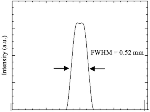
Profile of the point spot flux used in the experiment. From the geometry of the experimental setup, the point spot flux has a FWHM of 0.52 mm.

All 64 channels from the multi-anode, flat-panel PMT were acquired for each coincidence event. Two 32-channel CAEN ADC cards (N792 ADCs, CAEN, Italy) were used for data acquisition.

Raw data were processed in the same manner as in (Ling et al 2006). We applied an energy window of ±20% around the photopeak to select 511 keV events that were photoelectrically absorbed in the crystal, as shown in figure 2.

Figure 2.

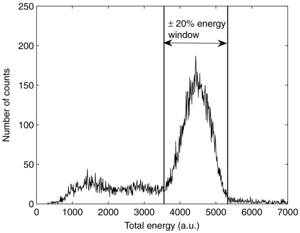
Energy window of ±20% around the photopeak.

Because of its stochastic nature, it is not possible to obtain a testing data set with the known spatial position (x, y) and DOI for each event at the same time. Most DOI calibration processes use an incident photon flux on the side of the crystal, which offers relatively good control over DOI. However because of the dimensions of our crystal, this methodology would only allow us to test a small fraction of the crystal along its edge and not the center section of the detector.

Therefore, for testing we adjusted the point photon flux to a 45° incidence angle relative to the crystal surface along the X-axis, as shown in figure 3. Thus, ideally DOI can be inferred by the x coordinate of the positioned event. An advantage of this acquisition scheme is that we can obtain data sets at any section of the crystal. A second set of data to evaluate our DOI method was collected on the same quarter of the crystal as the first one. Data were collected on a 11 × 11 grid with ∼1 mm spacing in both axes in the center and corner regions of the detector. Energy windowing as described above was also applied to the data. No other windowing was applied to the testing data.

Figure 3.

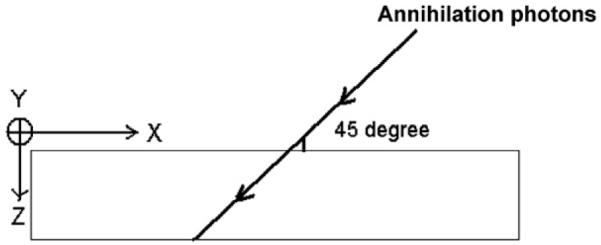
An annihilation photon beam incident at 45° relative to the surface. The depth of the first photon interaction in the crystal is equal to the spatial position along the X-axis.

2.2. Positioning algorithm

2.2.1. Light distribution models

The parametric positioning proposed here was based on modeling the light distribution with a Cauchy, Gaussian or parametric model. The assumption was that for single photoelectric absorption events, the probability of the light photons reaching the ith PMT channel is only a function of the spatial position (x, y, z) of the event. The function was assumed to take the form of the Cauchy (equation (1)), Gaussian (equation (2)) or parametric model (equation (3)):

$$p_i(x,y,z)=\frac{a\left(z\right)b{\left(z\right)}^2}{{(x-x_i)}^2+{(y-y_i)}^2+b^2\left(z\right)},$$ (1)

$$p_i(x,y,z)=a\left(z\right)\exp \left[-\frac{{(x-x_i)}^2+{(y-y_i)}^2}{b^2\left(z\right)}\right],$$ (2)

$$p_i(x,y,z)=a\left(z\right){\left(1+\frac{{(x-x_i)}^2+{(y-y_i)}^2}{b{\left(z\right)}^2\gamma }\right)}^{-\gamma }$$ (3)

(x_i, y_i are the position of the ith PMT channel.)

The symmetry between x and y in the equations reflects the fact that the light photons are released isotropically from the photoelectric absorption site. The choice of the Cauchy model (equation (1)) is inspired by the relationship between the solid angle subtended by a square and its distance from the center. The Gaussian model (equation (2)) is adapted from (Antich et al 2002) for comparison purposes. The parametric model is a more general form of the first two models. If γ = 1, the parametric model is just the Cauchy model; if γ → ∞, the parametric model will converge to the Gaussian model. In all these models, a is the peak value of the light distribution and b characterizes the light spread.

The translational invariance of the function on the X-Y plane reveals the underlying assumption of no edge reflection effect, so a and b depend only on z. Since we do not know the functional form of a(z) and b(z), the actual variables in the equations above are (x, y, a, b) in equations (1) and (2) or (x, y, a, b, γ) in equation (3).

Sample p_i curves from the three models are plotted in figure 4. In the plots x_i and y_i are set to zero, b to 6, γ to 2 and the height is normalized.

Figure 4.

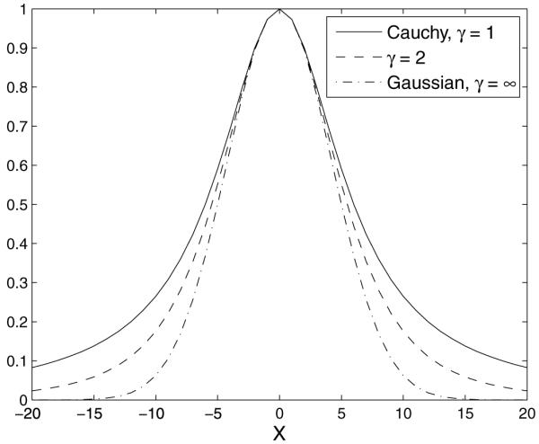
Comparison of the Cauchy, Gaussian and parametric models. The Cauchy model has a longer tail than the Gaussian. The parametric model is versatile to fit a wide variety of tails.

2.2.2. Model fitting

Two methods were used to fit the models: maximum-likelihood estimation (MLE) and weighted least-squares (WLS).

1. MLE. If N, the number of light photons generated in a photoelectric interaction event, is fixed, the distribution of photons among the number PMT channels n_i, i = 1, 2, . . . , 64, and the number of photons escaping $(N-{\sum }_{i=1}^{64}{n}_i)$ follows a joint multi-nomial distribution, and the marginal distribution of n_i can be approximated by a Poisson distribution with λ_i = N · p_i. Suppose the PMT quantum efficiency is a constant Q, then the number of light photons generating signal in PMT channel $n_i^{\ast }$ still follows a Poisson distribution with λ_i = QN · p_i, then the actual signal we collect is $m_i=M{n}_i^{\ast }$, if M is the gain of an ideal noiseless PMT.

   Furthermore, we assume that the correlation between $n_i^{\ast }$ and $n_j^{\ast }$ is negligible for i ≠ j, so $n_i^{\ast }$ follow independent Poisson distributions. The likelihood function of observation m_i, i = 1, 2, . . . , 64, as a function of (a, b, x, y, (γ)) is

   $$f(\left(m_i\right)\mid a,b,x,y,\left(\gamma \right))=\prod _{i=1}^{64}L({\lambda }_i\mid n_i^{\ast })=\prod _{i=1}^{64}\frac{e^{-{\lambda }_i}{\lambda }_i^{n_i^{\ast }}}{n_i^{\ast }!}.$$ (4)
   The log-likelihood function is

   $$\ln L(a,b,x,y,\left(\gamma \right))=\sum _{i=1}^{64}(n_i^{\ast }\ln {\lambda }_i-{\lambda }_i-\ln n_i^{\ast }!).$$ (5)
   After plugging in the variables, the above equation can be simplified to

   $$\ln L=\frac{1}{M}\sum _{i=1}^{64}(m_i\ln \left(MQN{p}_i\right)-MQN{p}_i)+\mathrm{const}.$$ (6)
   If we define $p_i^{\ast }=MQN{p}_i$ and a* = MNQa, then the maximum-likelihood estimator is given by

   $$(\widehat{a},\widehat{b},\widehat{x},\widehat{y},\left(\widehat{\gamma }\right))=\underset{(a,b,x,y,\left(\gamma \right))}{\mathrm{argmax}}\ln L=\underset{(a,b,x,y,\left(\gamma \right))}{\mathrm{argmax}}\frac{1}{M}\sum _{i=1}^{64}(m_i\ln p_i^{\ast }-p_i^{\ast }),$$ (7)

   which is equivalent to

   $$({\widehat{a}}^{\ast },\widehat{b},\widehat{x},\widehat{y},\left(\widehat{\gamma }\right))=\underset{(a^{\ast },b,x,y,\left(\gamma \right))}{\mathrm{argmax}}\ln L=\underset{(a^{\ast },b,x,y,\left(\gamma \right))}{\mathrm{argmax}}\frac{1}{M}\sum _{i=1}^{64}(m_i\ln p_i^{\ast }-p_i^{\ast }).$$ (8)

   The only difference is that a is replaced by a*. The ML estimation is independent of the numerical value of M, Q and N, which greatly simplifies the problem, since M, Q and N are not straightforward to be determined and vary as the environment changes.

2. WLS. Referring to the assumption and analysis above, a reasonable WLS would be

   $$(\widehat{a},\widehat{b},\widehat{x},\widehat{y},\left(\widehat{\gamma }\right))=\underset{(a,b,x,y,\left(\gamma \right))}{\mathrm{argmin}}\sum _{i=1}^{64}\frac{{(n_i^{\ast }-{\lambda }_i)}^2}{{\lambda }_i},$$ (9)

   where λ_i is chosen as the weight of the square errors.
   It is easily shown that the above WLS can be also expressed as

   $$(\widehat{a},\widehat{b},\widehat{x},\widehat{y},\left(\widehat{\gamma }\right))=\underset{(a,b,x,y,\left(\gamma \right))}{\mathrm{argmin}}\sum _{i=1}^{64}\frac{{(m_i-p_i^{\ast })}^2}{M{p}_i^{\ast }},$$ (10)

   which is equivalent to the following:

   $$(\widehat{a},\widehat{b},\widehat{x},\widehat{y},\left(\widehat{\gamma }\right))=\underset{(a,b,x,y,\left(\gamma \right))}{\mathrm{argmin}}\sum _{i=1}^{64}\frac{{(m_i-p_i^{\ast })}^2}{p_i^{\ast }}.$$ (11)

   From the analysis above, $n_i^{\ast }$ follows a Poisson (λ_i) distribution. Therefore, both the mean and variance are equal to λ_i. The normal distribution is a good approximation when λ is not small (>10).

   Comparing to MLE, WLS offers several advantages: (i) although the choice of weight is based on the assumption and analysis of MLE, no particular assumption, such as the Poisson distribution, is needed for the validity of this method and (ii) the residue of WLS can be used to diagnose the goodness of fit of the model. Given the correct model, the sum of square residue (SSR) should follow a χ² probability density function (PDF) with degrees of freedom (df) 60 for the Cauchy and Gaussian models, and 59 for the parametric model. The residues for each channel should follow a standard normal distribution.

2.2.3. Depth-of-interaction decoding

From the assumption above, the parameters a, b and γ are functions of the depth-of-interaction Z. Though it is impossible to derive an analytic form for the functions, it is feasible to construct a linear estimator from a, b and γ: Z = β₀ + β₁a + β₂b for the Cauchy or Gaussian model and Z = β₀ + β₁a + β₂b² + β₃γ for the parametric model. The reason we use b², instead of b, will be clear in the results section.

In order to obtain the coefficients in the estimator, the data set acquired with the point flux tilted 45° along the X direction relative to the detector surface used, see figure 3. In this setup, Z_x, the distance between the estimated X position and the location where the point flux enters the detector, can be used to approximate DOI. By fitting the regression model Z_x = ∊ + β₀ + β₁a + β₂b or Z_x = ∊ + β₀ + β₁a + β₂b² + β₃γ to the experimental data, we canget the coefficients β_i. Thus the general estimator for DOI based on a, b, (γ), Z_ab(γ) can be calculated by Z_ab = β₀ + β₁a + β₂b or Z_abγ = β₀ + β₁a + β₂b² + β₃γ.

3. Results

3.1. Model selection

First, the goodness of fit of the three models was diagnosed using WLS. Histograms of SSR from the Cauchy and parametric models are shown in figure 5. The Gaussian results are not shown because the SSR from the Gaussian model was too large to fit in figure 5. The histograms were linearly rescaled by the same constant to fit the Chi-square distribution, since the objective function in WLS is rescaled by M. It is clear that the SSR from the parametric model is reasonably close to the χ² PDF (with df = 59), while SSR from the Cauchy and Gaussian models are large compared to the χ² PDF (df = 60). The histogram of γ in the parametric model is shown in figure 6. It centers at around γ = 1, which indicates that the Cauchy model might fit the data as well. But the significant reduction of SSR by the parametric model over the Cauchy model implies that the more general parametric model is required.

Figure 5.

The histogram of SSR versus χ² distribution. (a) SSR from the Cauchy model, along with χ² PDF with 60 degrees of freedom for comparison and (b) SSR from the Cauchy and parametric models, along with χ² PDF with 59 degrees of freedom. The solid lines indicate the 99% quantile of the corresponding χ² distribution.

Figure 6.

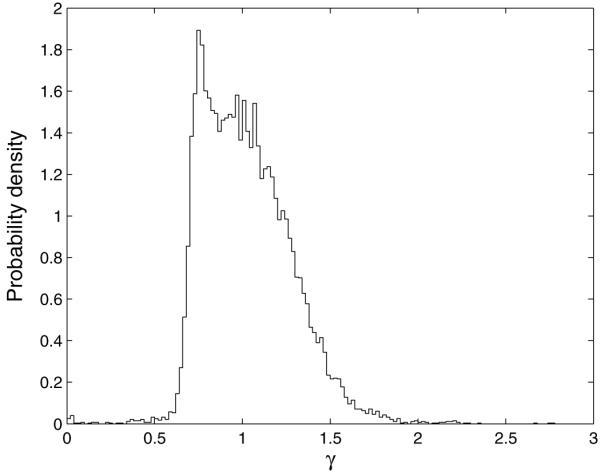
The histogram of γ for the parametric model. Though it centers at γ = 1, which corresponds to the Cauchy model, it has a relatively large spread over [0.5, 2].

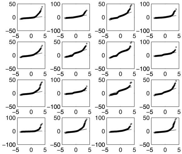
From the previous discussion, given the correct model, the residues from individual channels follow a standard normal distribution. QQ-plots are used to illustrate the normality of the residues using three different models, as shown in figures 7-9. Events with SSR larger than 95% level of the corresponding χ² distribution (df = 60 for the Cauchy model, df = 59 for the parametric model) are removed as outliers, except for the Gaussian model. The plots of the parametric model are very close to a straight line, which is the ideal plot for a standard normal distribution. This further confirmed that the parametric model is the best fit.

Figure 7.

Sample QQ-plots of the residues from individual channels using the Cauchy model: (a) all events and (b) after 95% χ² thresholding.

Figure 9.

Sample QQ-plots of the residues from individual channels using the parametric model: (a) all events and (b) after 95% χ² thresholding.

The sample Cauchy, Gaussian and parametric model fits to the same event are shown in figure 10. The exponential tail of the Gaussian distribution cannot match the long tail of the real data. Conversely, the Cauchy model is too heavily tailed. The parametric model is versatile to fit the data.

Figure 10.

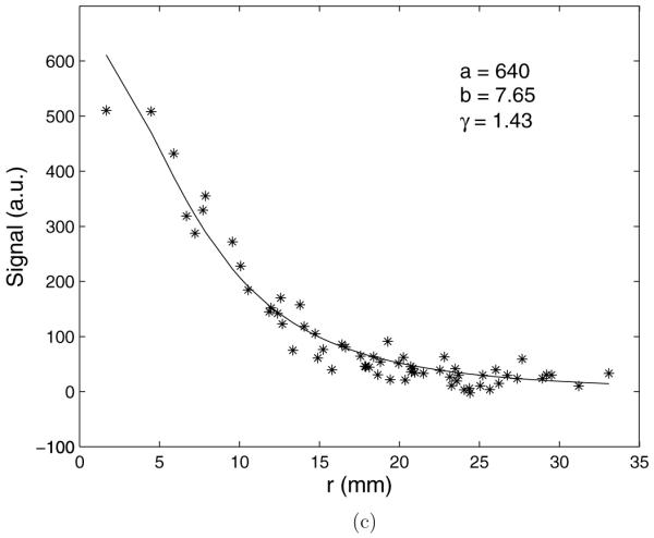
Fitted curve and a sample event versus distance from the estimated interaction location using (a) the Cauchy model, (b) the Gaussian model and (c) the parametric model.

The parametric model proved to be the best model to fit the real data. The rest of the reported results focus on the parametric model.

3.2. Intrinsic spatial resolution

The intrinsic spatial resolution was studied using the perpendicular test beam data set. A sample fitting result using MLE and parametric model is shown in figure 11.

Figure 11.

A sample positioning result of the perpendicular data set using MLE and parametric fit: (a) 3D mesh and (b) profile along the X-axis. The FWHM of the shown profile is 1.15 mm.

(This figure is in colour only in the electronic version)

For the testing data set, 13 × 13 data points were used to study the performance near the center of the crystal, and 11 × 11 for the corner section (to within ∼3.5 mm from the edge of the detector). Contour plots of the results using the MLE methodare shown in figure 12. The spacing between adjacent testing positions is 2 mm. The results for intrinsic resolution are summarized in table 1. The performance of the Cauchy and parametric models is clearly superior to the Gaussian model. The Gaussian model provides reasonable performance in the center region of the detector, but completely breaks down in the off-center region. The best intrinsic spatial resolution is achieved by the parametric model, which is 1.06 ± 0.21 mm at the center and 1.27 ± 0.48 mm at the corner.

Figure 12.

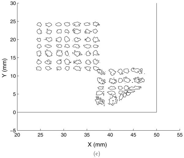
Contour plot illustrating the FWHM of positioning results using the MLE method with 2.0 mm center-to-center spacing to within 3.5 mm of the edge of the detector: (a) Cauchy model, (b) Gaussian model and (c) parametric model. The black lines indicate the crystal boundary.

Table 1.

Comparison of the intrinsic spatial resolutions and FWTM (full-width tenth-maximum) using different models

	Intrinsic spatial resolution (mm)		FWTM (mm)
Model	Center	Corner	Center	Corner
Parametric	1.06 ± 0.21	1.27 ± 0.48	2.81 ± 0.73	3.2 ± 1.4
Cauchy	1.11 ± 0.22	1.30 ± 0.34	2.91 ± 0.69	4.3 ± 1.8
Gaussian	1.28 ± 0.76	-	3.5 ± 1.4	-

3.3. Truncation versus reflection

Though the parametric model has superior performance in most regions on the detector, it has severe bias near the corner. There are two possible reasons for the bias:

1. reflection; because of light reflection from the edges of the crystal, the translational invariance assumption of the parametric model no longer holds;

2. truncation; because of the loss of light collection, the information about the scintillation location contained in the PMT signals is also lost.

In order to decouple the two effects, we excluded the last row and column of PMT channels in the positioning process, which is equivalent to creating a virtual corner without edge reflection. We used three data points near the virtual corner for testing. The contours at half maximum of the positioning results are plotted in figure 13. The straight lines indicate the virtual corner. The contours near the corner were processed using all 64 PMT channels; the ones at the center were the same data, but processed using 49 channels. We observed the similar bias pattern, as appears in the real corner of the detector, as shown in figure 12(c). It proves that the truncation effect, i.e., missing the last row and column of PMT channels, is the dominant reason for the bias in the positioning result.

Figure 13.

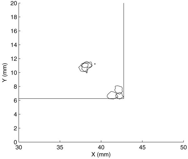
Contour plot at FWHM of the positioning results using all 64 PMT channels and 49 channels. The straight lines indicate the virtual corner, created by excluding the last row and column of PMT channels. Points near the virtual corner correspond to using all 64 PMT channels. Positioning is severely biased when using only 49 PMT channels.

3.4. DOI performance

The 45° angle incident data were fit using the parametric model and the Cauchy model with MLE. Since the flux was incident at a 45° angle relative to the surface of the crystal along the X-axis, we would expect that all events should have the same Y position, whereas they should be spread out along the X-axis. This was confirmed by the projection curves for the X- and Y-axes, shown in figure 14. The interaction region in X is determined by the 8 mm range including the most number of events. The interaction region along the Y-axis is chosen to be 2 mm wide, slightly larger than the sum of the source size and the intrinsic spatial resolution. The relatively heavy tail of the projection in the Y-axis is caused by a slight misalignment between the incident beam and the X- and Y-axes. Only events within this region were kept for DOI parameter fitting, as discussed below. All events were used to evaluate the DOI performance.

Figure 14.

A sample projection of the positioning result of the 45° incident data set, using MLE fit and the parametric model along the X- and Y-axes. Only the events within the range in both the X- and Y-axes as indicated by dashed lines, were used for DOI analysis.

Sample scatter plots of Z_x versus a, b or γ from the parametric model are shown in figure 15. The apparent correlations confirm the assumption that a, b and γ are functions of Z. Therefore, they can be used to estimate Z.

Figure 15.

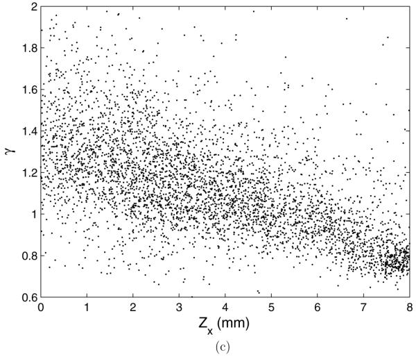
A sample scatter plot of Z_x versus a, Z_x versus b and Z_x versus γ using MLE parametric model fit. Z_x refers to the DOI (Z) calculated from the X position. Only data in the interaction region are plotted.

Following the coefficient fitting method discussed above, a set of β_i is fit at each calibration spot. Z_ab(γ) can be calculated using the corresponding a, b and γ. The difference between Z_ab(γ) and Z_x is considered the uncertainty of this estimation technique.

The best DOI result is achieved by Z_abγ using the parametric model. A sample histogram of the difference between Z_abγ and Z_x is shown in figure 16. The DOI resolution is estimated to be 3.24 ± 0.36 mm by averaging the FWHM of the histograms of the 45° incident testing data set. If the coefficients β₁ and β₂ are fixed to the average across all testing locations, the DOI resolution degraded to 3.54 ± 0.44 mm, which means β₁ and β₂ are relatively stable across the detector surface. Therefore, it is possible to simplify the DOI estimation process by using the same set of coefficients for all different positions on the detector.

Figure 16.

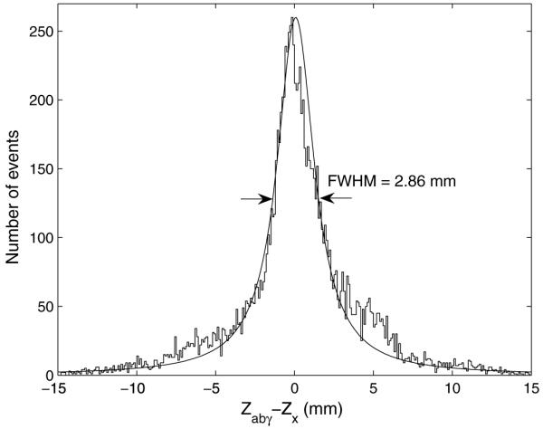
The difference between the DOI calculated by the x-coordinate and DOI from (a, b, γ). All data are plotted.

A similar DOI estimation was also carried out using the Cauchy model, using a and b as predictors for DOI. As shown in figure 17(a), the correlations between Z_x and a and b are less obvious than the parametric model, which in turn, explains why the DOI resolution using the Cauchy model is 4.72 ± 0.58 mm, considerably worse than the results using the parametric model.

Figure 17.

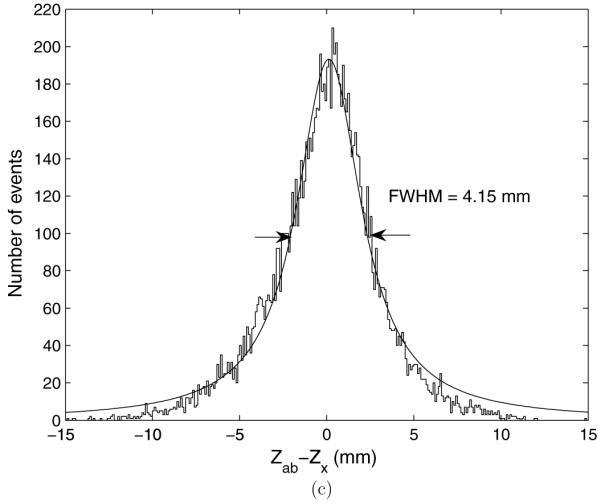
DOI estimation using the MLE Cauchy model fit: (a and b) a sample scatter plot of Z_x versus a and Z_x versus b and (c) the uncertainty in estimating DOI.

4. Conclusion

We have demonstrated a parametric method to determine the position and DOI on a continuous crystal detector. The intrinsic spatial resolution is estimated to be 1.06 mm and 1.27 mm FWHM at the center and corner (∼3.5 mm from the edge of the detector) sections of the detector, respectively. The parameters for the light spread and height are used to predict DOI. A DOI resolution of ∼3.24 mm FWHM is achieved. Because the finite testing source size and the uncertainty of using spatial position as a proxy for DOI have not been deconvolved, the true DOI resolution is actually better. The parametric nature of this method avoids the time-consuming calibration of the detector, as was required for the SBP method to generate lookup tables.

Even at corner sections, the parametric model resulted in small FWHM, but had large bias, which degraded the intrinsic spatial resolution measure. Further investigation shows that the truncation effect is the dominant factor for the estimator bias. This fact suggests that an unbiased estimator may not exist in this particular region and improving the light model by incorporating the edge reflection may not lead to a significant improvement.

While the initial hope was that the parametric positioning method would not require calibration, in order to use the method a bias correction LUT will be required for the corner sections of the detector. For a useful imaging area of 44 mm × 44 mm this will require calibrating a 6 mm × 6 mm region in each corner of the detector. Based upon results from our SBP method, this will require 16 (4 × 4 array) sample points for each corner of the detector or 64 calibration points in total. In comparison, our SBP method requires a total of 625 (25 × 25 array) sample points to characterize the same size detector.

A 44 mm × 44 mm useful imaging area is equivalent to a linear packing fraction of 88%. This is equivalent to a discrete crystal detector array with 1.4 mm × 1.4 mm cross-section crystals and 1.6 mm pitch (i.e., center-to-center distance between crystals). Most modern discrete crystal detector blocks have linear packing fractions better than 92%. To improve the effective detector packing fraction, a larger detector imaging area can be used with a sacrifice in the intrinsic spatial resolution for the edges and corners of the crystal. Thus there is a tradeoff between the overall intrinsic spatial resolution and sensitivity. A second approach to improve the effective packing fraction is to go to a trapezoid crystal geometry as suggested by (Benlloch et al 2007). Investigating a trapezoidal crystal implementation is planned for future work.

For human imaging systems, future studies will need to be carried out to determine detector characteristics using our parametric positioning approach on thicker crystal detectors. One advantage for a human detector system is that the intrinsic spatial resolution requirements are not as high as required for a small animal imaging system. While our goals were to achieve an intrinsic spatial resolution better than 1.4 mm FWHM for small animal imaging applications, an intrinsic spatial resolution of 4-6 mm FWHM is acceptable for human whole body systems. By relaxing the intrinsic spatial resolution requirements, it is feasible that the useful imaging area of the detector will approach 100%.

While edge effects may ultimately limit this approach, PET detectors that are capable of providing depth of interaction information can have a significant impact on future PET detector designs. For commercial human PET systems, detectors that provide some DOI information will allow systems to be built with smaller ring diameters. Having a smaller ring diameter will translate into lower cost scanners or scanners with longer axial field of view. A scanner with longer axial field of view can shorten the imaging time for patient studies. For speciality PET systems that require ultra-high spatial resolution (e.g. <2 mm FWHM) detectors that provide some DOI information can lead to scanners with much higher detector efficiency. This is especially important for small animal imaging systems where the injected dose may be significantly limited by the specific activity of the labeled compound (e.g. for receptor imaging studies).

Figure 8.

Sample QQ-plots of the residues from individual channels using the Gaussian model.

References

- Antich P, Malakhov N, Parkey R, Slavin N, Tsyganov E. 3D position readout from thick scintillators. Nucl. Instrum. Methods A. 2002;480:782–7. [Google Scholar]
- Benlloch JM, et al. Scanner calibration of a small animal PET camera based on continuous LSO crystals and flat panel PSPMTs. Nucl. Instrum. Methods A. 2007;571:26–9. [Google Scholar]
- Cherry SR, et al. MicroPET: a high resolution PET scanner for imaging small animals. IEEE Trans. Nucl. Sci. 1997;44:1161–6. [Google Scholar]
- Clinthorne NH, Rogers WL, Shao L, Koral KF. A hybrid maximum likelihood position computer for scintillation cameras. IEEE Trans. Nucl. Sci. 1987;34:97–101. [Google Scholar]
- Dahlbom M, Hoffman EJ. An evaluation of a two-dimensional array detector for high resolution PET. IEEE Trans. Med. Imaging. 1988;7:263–72. doi: 10.1109/42.14508. [DOI] [PubMed] [Google Scholar]
- Del Guerra A, Domenico GD, Scandola M, Zavattini G. YAP-PET: first results of a small animal positron emission tomography based on YAP:Ce finger crystals. IEEE Trans. Nucl. Sci. 1998;45:3105–8. [Google Scholar]
- Gray RM, Macovski A. Maximum a posteriori estimation of position in scintillation cameras. IEEE Trans. Nucl. Sci. 1976;23:849–52. [Google Scholar]
- Joung J, Miyaoka RS, Lewellen TK. cMiCE: a highresolution animal PET using continuous LSO with a statistics based positioning scheme. Nucl. Instrum. Methods A. 2002;489:584. [Google Scholar]
- Ling T, Lee K, Miyaoka RS. Performance comparisons of continuous miniature crystal element (cMiCE) detectors. IEEE Trans. Nucl. Sci. 2006;53:2513–8. [Google Scholar]
- Ling T, Lewellen TK, Miyaoka RS. Depth of interaction decoding of a continuous crystal detector module. Phys. Med. Biol. 2007;52:2213–28. doi: 10.1088/0031-9155/52/8/012. [DOI] [PubMed] [Google Scholar]
- Milster TD, Aarsvold JN, Barrett HH, Landesman AL, Mar LS, Patton DD, Roney TJ, Rowe RK, Seacat RH., III A full-field modular gamma camera. J. Nucl. Med. 1990;31:632–9. [PubMed] [Google Scholar]
- Miyaoka RS, Janes M, Lee K, Park B, Kinahan P, Lewellen T. Toward the development of a micro crystal element scanner (MiCES): quickpet II. Mol. Imaging. 2005;4:117–27. doi: 10.1162/15353500200504154. [DOI] [PubMed] [Google Scholar]
- Seidel J, Vaquero JJ, Green MV. Resolution uniformity and sensitivity of the NIH ATLAS small animal PET scanner: comparison to simulated LSO scanners without depth-of-interaction capability. IEEE Trans. Nucl. Sci. 2003;50:1347–50. [Google Scholar]
- Surti S, Karp JS, Perkins AE, Freifelder R, Muehllehner G. Design evaluation of A-PET: A high sensitivity animal PET camera. IEEE Trans. Nucl. Sci. 2003;50:1357–63. [Google Scholar]
- Tai YC, Chatziioannou AF, Yang YF, Silverman RW, Meadors K, Siegel S, Newport DF, Stickel JR, Cherry SR. MicroPET II: design, development and initial performance of an improved MicroPET scanner for small-animal imaging. Phys. Med. Biol. 2003;48:1519–37. doi: 10.1088/0031-9155/48/11/303. [DOI] [PubMed] [Google Scholar]
- Ziemons K, et al. The ClearPET project: development of a 2nd generation high-performance small animal PET scanner. Nucl. Instrum. Methods Phys. Res. A. 2005;537:307–11. [Google Scholar]