

Abstract
The Lumry-Eyring with nucleated-polymerization (LENP) model from part 1 (Andrews and Roberts, J. Phys. Chem. B 2007, 111, 7897 7913) is expanded to explicitly account for kinetic contributions from aggregate-aggregate condensation polymerization. Experimentally accessible quantities described by the resulting model include monomer mass fraction (m), weight-average molecular weight (Mw), and ratio of Mw to number-average molecular weight (Mn) as a function of time (t). Analysis of global model behavior illustrates ways to identify which steps in the overall aggregation process are kinetically important, based on the qualitative behavior of m, Mw, and Mw/Mn vs. t, and based on whether bulk phase separation or precipitation occurs. For cases in which all aggregates remain soluble, moment equations are provided that permit straightforward numerical regression of experimental data to give separate time scales or inverse rate coefficients for nucleation and for growth by chain and condensation polymerization. Analysis of simulated data indicates that it may be possible to neglect condensation reactions if only early-time data are considered, and also highlights difficulties in conclusively distinguishing between alternative mechanisms of condensation even when kinetics are monitored with both m and wM.
Keywords: non-native aggregation, mathematical modeling, protein stability
1. Introduction
Non-native aggregation commonly refers to the process of forming protein aggregates in which the constituent monomers have significantly altered secondary structure compared to the native or folded state.1-3 Aggregates may be soluble or insoluble, with soluble aggregates potentially ranging in size from dimers to so called high molecular weight species (~ 10 - 103 or more monomers per aggregate).4-6 Formation of non-native aggregates is problematic for protein based pharmaceuticals and other biotechnology products due to increased manufacturing costs, regulatory concerns, and product marketability.3,6-8 Non-native aggregates are also implicated in a number of chronic diseases9,10 and are suspected immunogenic agents in biopharmaceuticals.11,12
Because non-native aggregation (hereafter referred to simply as aggregation) is typically net irreversible under the conditions that aggregates form, elucidating key mechanistic details that control aggregation kinetics is of general importance for these systems. However, even apparently simple experimental kinetics can be a convolution of multiple stages.2 These may include: (partial) monomer unfolding; reversible self association or pre nucleation; nucleation of the smallest irreversible aggregates; and subsequent aggregate growth via chain polymerization and/or aggregate self association or phase separation. Furthermore, many of the kinetically relevant intermediates are often too poorly populated or transient to be directly characterized with available experimental methods.2,6,13,14 As a result, proper deconvolution of different stages of the aggregation process requires qualitative and quantitative comparison with mechanistic mathematical models that are couched in experimentally accessible quantities such as mass-percent loss of monomer and time-dependent scattering data.2,4,15-19
A large majority of available mathematical models for aggregation kinetics can be categorized in terms of which stage or stages in the overall aggregation process that they treat explicitly or implicitly. Currently, no available model treats all of the above stages with equally detailed descriptions for natively folded proteins. Rather, most models fall in one of two categories.2 Those in the spirit of Lumry-Eyring treatments primarily consider only unfolding and folding in mechanistic detail, and use phenomenological or empirical treatments for assembly steps. Alternatively, polymerization models typically ignore conformational transitions and treat only assembly steps in detail.2
A previous report20 presented a first generation Lumry-Eyring Nucleated-Polymerization (LENP) model that included thermodynamics of monomer conformational stability and prenucleation, along with dynamics of nucleation and of growth via chain polymerization. It is also one of only two models20-22 that consider the effects of aggregate (in)solubility on experimental kinetics of monomer loss or soluble-aggregate size distributions. In this context, soluble aggregates are those that are available to consume additional protein monomers,15-24 rather than being defined in terms of a particular size range.25
The previous LENP model did not include detailed treatments of the kinetics and mechanism of aggregate-aggregate coalescence or condensation leading to soluble and/or insoluble aggregates.2,20,22 Incorporating details of condensation is important if one is interested in quantifying the resulting aggregate size distribution, but can lead to significant added mathematical complexity.26 This may explain why, for non-native protein aggregation, there are relatively few experimentally tested kinetic models that describe condensation in considerable detail, and those models have typically been system-specific.
For example, Pallitto and Murphy incorporated size-dependent, diffusion limited lateral and end to end association to describe soluble filament and insoluble fibril formation based on a priori knowledge of stoichiometry and geometry in Aβ aggregation.16 In simpler treatments, Modler et al17 and Speed et al18 considered irreversible condensation polymerization to form soluble aggregates, with rate coefficients that were assumed to be independent of polymer size (degree of polymerization). In each case, kinetic models were regressed against time-dependent measurements of one or more aspects of the aggregate size distribution, e.g., weight-average molecular weight16-18 or z-average hydrodynamic radius.16 Condensation was determined to be an important or even dominant contribution in each case. However, in each case the models were developed for only a specific protein system, without considering global model behavior.
Furthermore, it is also common practice to fit monomer loss data to models in which condensation is inherently neglected,15,23,27,28 even though corroborating structural evidence to support such an assumption may be available in only a fraction of reported cases.2,6 Overall, this highlights a need for more general analysis of aggregation kinetics within a mechanistic framework that can easily distinguish which contributions are important, and that can also provide a means to quantify those contributions by regression against experimental kinetics.
The present report extends the previous LENP model to include explicit and detailed descriptions of condensation. Particular questions that are addressed include: (1) what experimental signatures easily allow one to qualitatively determine whether neglecting condensation20,23,24,27-29 is appropriate? (2) can one quantitatively separate contributions from condensation, chain-polymerization, and nucleation without detailed a priori knowledge16 of the association mechanism or aggregate morphology? (3) how sensitive are experimentally accessible kinetics to mechanistic details such as size-dependent vs. size-independent condensation steps? (4) how are the answers for (1) to (3) altered if one considers only early-time data (i.e., only the first few percent loss of monomer)? These questions are important for deconvoluting the effects of chemical additives or protein stabilization strategies on different stages of aggregation,2,30-32 inferring mechanistic details of aggregate-aggregate assembly,16 and in applications such pharmaceutical product stability that typically focus on only small extents of reaction or percent loss of monomer.3,6 Finally, this report provides the global behavior of the improved LENP model, and illustrates an application of the model to experimental data using recently reported results for aggregation of α-chymotrypsinogen A (aCgn).5
2. Model Description & Derivations
Table 1 summarizes key symbols and definitions used throughout this report. Fig. 1 schematically shows the six stages of nonnative aggregation that are included in the model developed and analyzed here. Stages 1 to 4 are the same as those employed in the previous LENP model.20 Briefly, the six stages in Fig. 1 are: (1) conformational transitions of monomers between folded (F) and unfolded (U) states, with the possibility for stable folding intermediates (I). The monomer conformational state (e.g., F, I, or U) that is most prone or reactive with respect to aggregation is denoted R; (2) association of R monomers to form reversible prenuclei or oligomers (Ri) composed of i molecules; (3) nucleation of the smallest aggregate species that is effectively irreversible (Ax) by a conformational rearrangement step (Rx → Ax);16,20 (4) growth of soluble aggregates via chain polymerization; (5) soluble aggregate growth due to aggregate-aggregate association such as condensation polymerization;5,16 (6) removal of aggregates via phase separation to form macroscopic particles or precipitates.21,33,34 In stage 6, all aggregates composed of n* or more monomers are treated as insoluble.20-22
Table 1.
List of key symbols
| Name | Definition |
|---|---|
| Aj | Agg. composed of j monomers(a) |
| Ax | Nucleus(a) |
| aj | [Aj]/C0 |
| C0 | Initial monomer concentration(a) |
| Cref | Std. state monomer conc.(a) |
| KIU | Eq. const, for I ↔ U |
| Ki | Eq. const, for iR ↔ Ri(b) |
| KNI | Eq. const, for N ↔ I |
| KRA | Eq. const, for Aj+R ↔ AjR(c) |
| ka | Monomer assoc. rate coeff.(d) |
| ka,x | ka for nucleation step(d) |
| kB | Boltzmann's constant(e) |
| kd | Dissociation rate coeff.(f) |
| kd,x | kd for Rx-1 + R ↔ Rx (f) |
| kg | Growth rate coeff.(d) |
| knuc | Nucleation rate coeff.(f) |
| kobs | Observed rate coeff. for monomer loss(f) |
| v | Apparent reaction order for monomer loss |
| δ | # monomers added per chain-polymerization step |
| kr | Rearrangement rate coeff.(f) |
| kr,x | kr for nucleation step(f) |
| ki,j | Condensation rate coeff.(d) |
| κi,j | ki,j/kx,x |
| τg | Characteristic timescale of chain polymerization |
| τn | Characteristic timescale of nucleation |
| τc | Characteristic timescale of condensation polymerization |
| N | Native monomer(a) |
| I | Intermediate state (monomer)(a) |
| U | Unfolded state (monomer)(a) |
| R | Reactive monomer(a) |
| fR | Fraction reactive monomer |
| n* | Size at which precipitation occurs |
| Ri | Reversible oligomer of i monomers(a) |
| Rx | Reversible prenucleus(a) |
| x | Nucleus stoichiometry |
| m | ([N]+[I]+[U])/C0 |
| Mnagg | Number-avg. aggregate MW(g) |
| Mmon | Monomer MW(g) |
| Mwagg | Weight-avg aggregate MW(g) |
| βgn | τn/τg |
| βcg | τg/τc |
| σ | Σ[Aj]/C0 |
| λ1 | 1st moment of soluble agg. size distribution |
| λ2 | 2nd moment of soluble agg. size distribution |
| θ | Dimensionless time (t/τn) |
| μ | Mean of aj/σ distribution |
| σμ | Variance of aj/σ distribution |
| Number average κi,j | |
| Weight average κi,j | |
| τg(0) | τg at Cref and fR = 1 |
| τn(0) | τn at Cref and fR = 1 |
| τc(0) | τc at Cref |
Abbreviations: agg. = aggregate, aggn. = aggregation, conc. = concentration, const. = constant, eq. = equilibrium, MW = molecular weight, unf. = unfolding
[mol/volume]
[(mol/volume)1-i]
[(mol/volume)-1]
[(mol/volume)-1·time-1]
[energy/K]
[time-1]
[mass·mol-1]
[Kelvin]
[time]
[energy/mol]
Figure 1.

Reaction scheme with associated model parameters for the six key stages in the LENP model. The steps shown in each panel are treated as elementary irreversible (single arrow) steps, or as pre equilibrated or steady-state (double arrow) when translating them to mass action kinetic equations.
As in the previous report,20 stages 1 and 2 are assumed to be fast and thus preequilibrated compared to stages 3-6. As a result, only equilibrium constants for unfolding (KFI, etc.) and prenucleation (Ki, i = 2,…,x-1) appear in stages 1 and 2, respectively. The kinetics of conformational rearrangement as part of nucleation in stage 3 are treated by assuming a concerted, unimolecular rate-limiting step with rate coefficient kr,x.20 The balance of rearrangement (Rx → Ax) and association (R + Rx-1 → Rx) steps in stage 3 is treated with a local steady-state approximation. For association, ka,x and kd,x denote forward and reverse rate coefficients. Similar considerations and nomenclature are included for growth via chain polymerization (stage 4).20 R monomers can reversibly self associate with pre-existing soluble aggregates, followed by a conformational rearrangement step that makes monomer addition effectively irreversible. The rate coefficients ka, kd, kr and equilibrium constant KRA in stage 4 are the same as in the earlier LENP model.20 In stage 5, ki,j denotes the rate coefficient for irreversible association of aggregates composed of i and j monomers to form a soluble aggregate of i + j monomers. Stage 6 is effectively instantaneous phase separation of any aggregate that contains n* or more monomers.
2.1 LENP model equations
The following derivations are based on the reaction scheme in Fig. 1, and employ the same nomenclature as previous work20 to the extent possible here. Characteristic time scales are defined for nucleation , growth via monomer addition , and condensation (see also Appendix). In these definitions, fR = [R]/([N]+[I]+[U]) is the mole fraction of monomer that is in the aggregation prone conformational state. Cref is a reference state concentration that defines the concentration scale of the standard state for association free energies and equilibrium constants. The respective intrinsic time scales (denoted with superscript (0)) are defined as , , and . They are termed intrinsic because they are independent of initial monomer concentration and the free energy of monomer conformational transitions. kg ≡ kakr/(kd + kr) is the effective rate coefficient for chain polymerization, and knuc ≡ ka,xkr,x/(kd,x + kr,x) is that for nucleation.20
The above definitions along with the derivations elsewhere20 and in the Appendix show that although there are numerous parameters in Fig. 1 and Table 1, the assumptions of preequilibration for stages 1 and 2, and local steady state for stages 3 and 4 reduce the total to only seven distinguishable parameters or functions: τn and x account for stages 1, 2, and 3; τg and δ account for stage 4; and n* accounts for stage 6. Stage 5 is accounted for by τc and κi,j ≡ ki,jC0τc. κi,j may be a function of i and j, but its (i,j) dependence is uniquely set by the choice of mechanistic model describing size-dependent condensation (see also below and Sec. 2.3). Therefore, there are six adjustable model parameters once the condensation mechanism is selected.
The Appendix provides additional details regarding derivations of the kinetic working equations for monomer and all soluble aggregates. Eqs. A1, A4, and A5 are the dynamic material balances based on Figure 1 and mass action kinetics. They can be rewritten in nondimensional form by defining θ = t/τn, βgn = τn/τg, and βcg = τg/τc to give
| (1) |
| (2) |
| (3) |
When i in Eq. 3 is odd, the right-most summation runs from x to (i-1)/2 instead of i/2. The dimensionless monomer concentration is m ≡ ([N]+[I]+[U])/C0, with contributions from [Ri] neglected for KiC0<<1;20 dimensionless concentrations for nuclei (ax ≡ [Ax]/C0) and larger irreversible aggregates (ai ≡ [Ai]/C0) are similarly defined. The dimensionless condensation rate coefficient is defined as κi,j (≡ ki,j/kx,x). If there is no size dependence for condensation, κi,j = 1 is a constant for all (i, j) pairs. The model parameters that determine the characteristic behavior of the solutions to Eq. 1-3 are [x,δ,κi,j,βgn,βcg,n*]. Eq. 1 is identical to the previous version of the LENP model.20 Eq. 2-3 are more complex than in the earlier model, as they include contributions from condensation (i.e., the terms in which βcg appears). If one neglects condensation (βcg = 0, τc → ∞), Eq. 2-3 are equivalent to the condensation free model in ref. 20.
In general, Eqs. 1-3 cannot be solved exactly in analytical form. They can be numerically integrated to simulate the time profiles for monomer concentration on a mass fraction basis (m), as well as the size distribution of aggregates and all associated moments of that distribution. The former quantity is often experimentally accessible by techniques such as size exclusion chromatography (SEC) and field flow fractionation (FFF).13,14,35 Indirect measures of m might also be useful, provided they can be properly calibrated against direct measurements.6 Examples include dye binding,36,37 changes in beta sheet content monitored spectroscopically,15,38,39 and turbidity or optical density (provided all aggregates are insoluble).34 In contrast, the detailed or precise size distribution (aj vs. j) is not usually accessible experimentally. However, techniques employing static or dynamic laser light scattering are able to provide exact or approximate values for the weight-average molecular weight (Mw) and the ratio of Mw to the number-average molecular weight (Mn). The ratio MwMn is the polydispersity of the size distribution.40 Using techniques such as SEC or FFF with in-line light scattering detection,5,13,35,41 it also possible to separately measure the weight-average molecular weight of the aggregate size distribution (), and to provide a lower bound on the polydispersity of that distribution, 5
Using the nomenclature here, the weight- and number-average molecular weights of soluble aggregates are
| (4a) |
| (4b) |
with Mmon denoting the molecular weight of a monomer, and the superscript agg indicating that the summations are carried out over all soluble species that do not assay as monomers. For the present case, this makes the lower bound j=x in the summations in Eq. 4. This is expected under conditions where prenuclei are thermodynamically disfavored (low values of KiC0).20 Equivalent expressions can be derived if one can experimentally resolve smaller aggregates or if it is not convenient to separate monomer contributions in the assay being employed.16-18,20
Eq. 4 also relates and to the first and second moments of the soluble aggregate size distribution (λ1 and λ2, respectively).
| (5a) |
| (5b) |
For n* → ∞, λ1 is equal to the fractional monomer loss (1-m) at a given time. The zeroth moment of the aggregate size distribution is equal to σ as it was defined previously20 (see also Appendix). Physically, σ is the total number of aggregates per unit volume, scaled by the initial protein concentration on a monomer basis. These moments are not normalized (e.g., σ is not 1). It follows from Eq. 4-5 that the polydispersity of the aggregate size distribution can be expressed as
| (6) |
2.2 Moment Equations for Soluble Aggregate Conditions
For cases where aggregates remain soluble throughout the course of an experiment (i.e., large n*), Eqs. 1-3 present an essentially infinite set of coupled, non linear ODEs. These must be repeatedly solved numerically to regress model parameters from experimental data unless one instead employs approximate, analytical solutions. Examples of accurate analytical solutions when condensation can be neglected were the focus of ref. 20 and have been previously used for regression against experimental data.4,15,19,42 However, those treatments do not provide a means to describe changes in the aggregate size distribution when condensation is appreciable.20 An alternative approach is to replace Eqs. 1-3 by summing across all aggregate sizes (j) to provide differential equations for the time dependence of m and different moments of the aggregate size distribution (see also Appendix). Under conditions where nucleation is slow compared to aggregate growth, Eqs. A4-A6 are accurate approximations, and with Eq. A1 lead to
| (7) |
| (8) |
| (9) |
with
| (10a) |
| (10b) |
and with the first moment (λ1 replaced by m. Eq. 10 defines number-average and weight-average κi,j values ( and , respectively). In the most general case, and are not constant because they depend on the aggregate distribution {aj}, and this distribution changes as aggregation proceeds. The simplest case mathematically is with and identical to unity at all times, and occurs when κi,j is independent of size.
Eq. 7-10, along with Eq. 4 provide a numerically tractable means for parameter estimation based on experimental kinetic data for monomer loss and aggregate molecular weight. However they are applicable only when all aggregates remain soluble. If appreciable aggregate phase separation (precipitation) occurs, Eq. 1-3 or simplified limiting cases such as shown below (Sec. 3) and elsewhere20 must instead be used.
2.3 A Simple Size-Dependent Condensation Model
As a test case to explore the effects of a physically plausible size dependence for κi,j, a difffusion-limited Smoluchowski model43,44 for aggregate association rates was selected (see also, Sec. 3.2).
| (11) |
NA is Avogadro's number; Di and Dj are the translational diffusion coefficients for aggregates composed of i and j monomers, respectively; Ri and Rj are the respective contact radii; and f is a steric factor that accounts for the fact that only a fraction of the surface of the aggregate(s) may be “reactive” with respect to contacting another aggregate. For simplicity, f was assumed to be independent of i and j, and the Stokes Einstein equation was applied for the translational diffusion coefficients. The resulting expression is
| (12) |
where kB is Boltzmann's constant, T is the absolute temperature, and η is the viscosity of the solvent. Analogous but more complex expressions can be derived by assuming different aggregate morphologies and/or details of the aggregate-aggregate association process.16,45 Using Eq. 12 in the definition of κi,j, and making the simplifying approximation that Rj ~ j gives
| (13) |
and are calculated based on the time-dependent aggregate size distribution {aj} as it is updated during numerical integration (see also Eq. 10). It is not possible to solve Eq. 7-10 with a size-dependent κi,j unless one assumes or knows the relationship between {aj} and the moments of the distribution. For illustration purposes here, simple discrete probability distribution functions (pdf) were used to describe the aggregate size distribution with mean (μ) and variance (σμ):
| (14a) |
| (14b) |
For under dispersed distributions (σμ < μ) the bionomial pdf was used, while for equal or overdispersed distributions (σμ ≥ μ) the negative bionomial pdf was used.46,47 In each case, the (normalized) pdf is completely specified by the mean and the variance, and these in turn are set by σ, λ1 (or m) and λ2.
Alternative models for the size dependence of κi,j and for pdfs to approximate the aggregate size distribution were also considered. However, a systematic study of each was foregone, as there are many possible alternatives and the purpose of considering a size-dependent κi,j in the present study was only to qualitatively assess the utility and limitations of using the simpler, size-independent κi,j approximation that is commonly used.17,18,21
3. Results & Discussion
Solutions to the LENP model (Eqs. 1-5) were simulated systematically over a wide range of model parameters, including: x = 2-10, βgn = 10-1 -103, βcg = 0-103, and n* = 10 to 2×10⁴ (effectively n*→∞). The value of δ was set as 1 for all simulated results reported below. Results for δ >1 were tested for selected conditions, and all derivations and resulting working equations below do not require δ=1 to be assumed. Additional parameter values beyond the extremes of the ranges listed above were also tested to confirm that no qualitative changes in behavior were observed by extending the parameter ranges. The initial conditions in each case were m = 1, σ = 0, aj = 0 (x ≤ j < n*).
Four main outputs from the model solutions are (each as a function of time): (1) monomer loss kinetics on a mass fraction basis, m(t) and dm/dt; (2) the zeroth moment or total number concentration of the aggregate size distribution, σ(t) and dσ/dt; (3) weight-average molecular weight of soluble aggregates, ; (4) aggregate polydispersity, . As noted in Sec. 2.1, outputs (1), (3), and (4) are directly or indirectly accessible in in vitro experiments. Typically, σ(t) is not directly accessible via experiment, but its behavior is a useful indicator of qualitatively distinct kinetic regimes 20 (see also below).
3.1 Global Model Behavior
Numerical solutions to the LENP model (Eq. 1-5) across a broad range of model parameter values with κi,j = 1 displayed qualitatively distinct regimes or types of behavior in terms of experimental observables. Table 2 summarizes the different types or categories of limiting behavior, using nomenclature based on previous reports.20,21 The type of qualitative behavior the model exhibits is dictated mathematically by the values of the five key dimensionless groups or parameters noted above (n*, x, δ, βgn, βcg). Figures 2 and 3 illustrate the qualitative behaviors in terms of m(t), σ(t), , and . Each of these quantities except σ can be experimentally determined quantitatively or semi quantitatively. The behavior of σ is included because it provides insight into the behavior of m(t) in each case. In Figures 2 and 3, t is scaled by t50 in order to more easily compare profiles with greatly different absolute time scales; t50 is defined by m(t = t50) = 0.5.
Table 2.
Summary of key experimental signatures and scaling behaviors for each kinetic type produced by the LENP model. Examples of illustrative profiles are given in Figures 2 and 3. Expanded from Ref. 20
| Kinetic Type | γ(a) | v(b) | α(c) | Polydispersity | |
|---|---|---|---|---|---|
| Ia | |||||
| Low βgn | x -1 | x | x | High | increases strongly and non-linearly with (1-m) |
| High βgn | x /2 | x /2+1 | x /2+1 | High | |
| Ib | x -1 | x | x | Insoluble Agg. / Precipitates Present | |
| Ic | x -1 | x | x | Low | ca. constant (= x) versus (1-m) |
| Id | Similar to Ic with small increase of polydispersity and | ||||
| II | (x + δ -1)/2 | δ | (x + δ)/2 | Low | linear in (1-m) |
| III(e) | x -1 | x, 1 | x, 1 | Insoluble Agg. / Precipitates Present | |
| IVa | Early time (< ca. t50) similar to Ic (low βgn) or II (high βgn) | ||||
| IVb | Early time (< ca. t50) similar to II; precipitates present at longer times. | ||||
| Type | Physical Scenario |
|---|---|
| Ia | Low βgn: nucleation-controlled monomer loss, condensation-dominated growth |
| High βgn: slow nucleation, competing condensation and chain polymerization | |
| Ib | polymerization to low-Mw, soluble aggregates with immediate precipitation |
| Ic | nucleation only; negligible chain polymerization, condensation, or precipitation |
| Id | nucleation with slow chain polymerization; negligible condensation or precipitation |
| II | slow nucleation, fast chain polymerization; negligible condensation or precipitation |
| III | type Ib with aggregates saturated at (finite) solubility limits |
| IVa | slow nucleation; condensation appreciable after t > ca. t50 |
| IVb | slow nucleation; fast polymerization; precipitation appreciable after t > ca. t50 |
γ defined by 1/t50 ~ kobs ~ (C0)γ
v defined by dm/dt = -kobsmv over ca. one or more half lives
α defined by kobs ~ fRα
Figure 2.
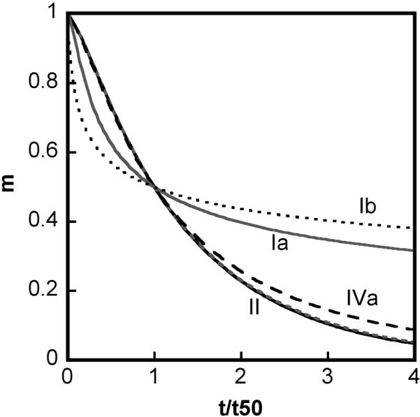
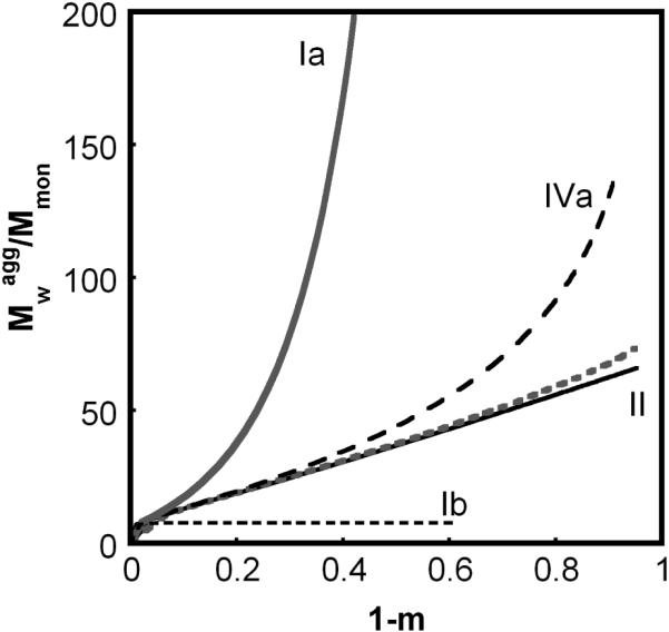


Illustrative profiles of limiting behaviors produced by the LENP model under conditions of fast chain polymerization relative to nucleation, based on simulations of Eq. 1-5 with βgn = 1000, x = 6, δ = 1, and for different regimes of n* and βcg. Qualitatively distinct behaviors are labeled according to the text in Section 3. Types Ia (solid gray), IVa (dash black), and II (both solid black and dotted gray) correspond to βcg = 10, 0.5, 0.05 and 0, respectively, with n* → ∞. Type Ib (dotted black) corresponds to βcg = 10 and n* = 10. The panels show (A) monomer loss kinetics, (B) as a function of the extent of reaction (1-m), (C) dimensionless number concentration (σ) of soluble aggregates available for further growth; (D) polydispersity of the aggregate size distribution as a function of (1-m). Polydispersity of type Ib is not shown, as experimental polydispersity results would be convoluted by the presence of insoluble/precipitating particles under type Ib conditions.
Figure 3.
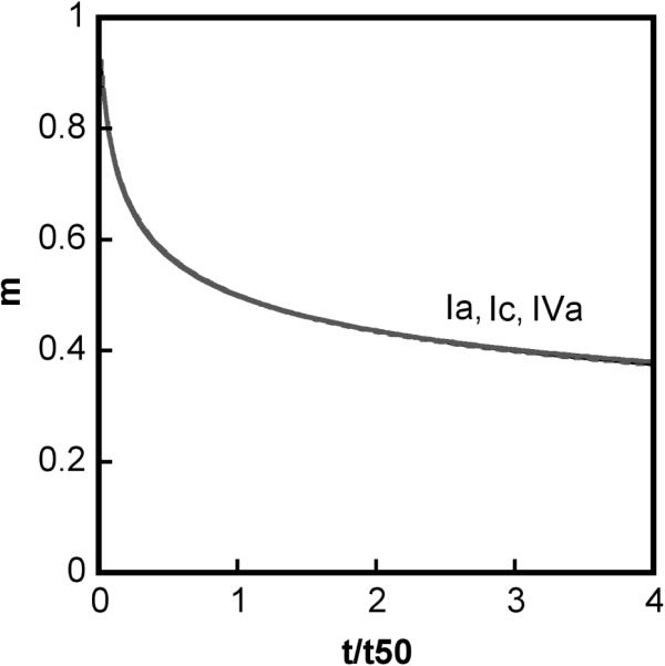
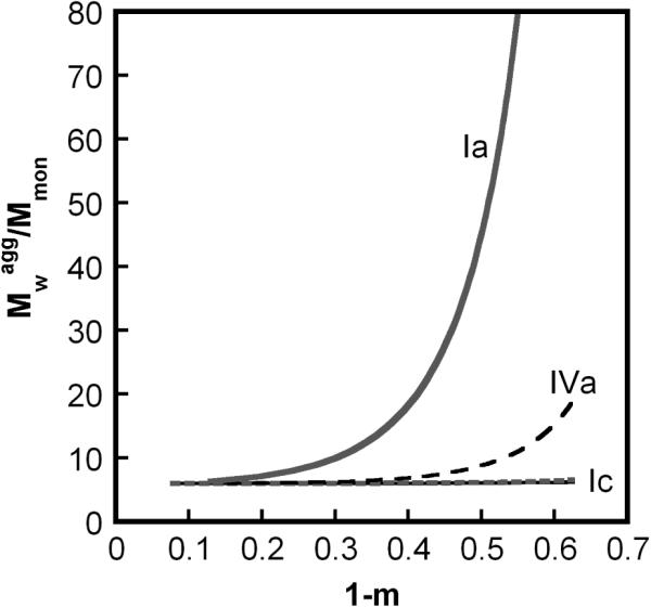


Analogous profiles to those in Figure 2, but under conditions of slow chain polymerization compared to nucleation; βgn = 0.1, other parameters are the same as in Fig. 2. Types Ia (solid gray), IVa (dash black), and Ic (both solid black and dotted gray) correspond to βcg at 1000, 50, and 0.01 and 0, respectively.
In Table 2, the scaling exponents correspond to limiting behaviors of the effective or observed rate coefficient for monomer loss (kobs) and apparent reaction order (v), defined by
| (15) |
when m(t) is considered over multiple half lives.20. The scaling relationships were derived previously20 for most entries in Table 2, and are included here for completeness when the new features are presented below. The primary new results are for the behavior of when comparing conditions where condensation is negligible or appreciable. The key features of types Ia, Ib, Ic, II, and IVa/IVb are briefly reviewed below. Type III occurs only if aggregate solubility limits are reasonably large,21 and is not reviewed further here. For reference, Figure 4 provides illustrative state diagrams that show ranges of model parameter values over which each kinetic type occurs. Each choice of parameter values for simulated profiles in Fig. 2 and 3 correspond to a state point in Figure 4.
Figure 4.

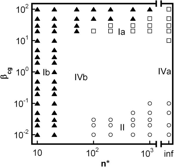
Kinetic state diagrams illustrating the placement of types Ia, Ib, Ic, II, and IVa/b within the space of model parameter values (x = 6, δ = 1, for all points). Panel A: varying βgn and βcg at fixed n* → ∞. Panel B: varying βcg and n* at fixed βgn = 1000. n* → ∞ (denoted as `inf') is also included for comparison; Different symbols denote different limiting case behaviors illustrated in Fig. 2, 3: Ia (open triangle), Ib (filled triangle), Ic (filled diamond), II (open circle). Types IVa/b (blank space) are intermediate behaviors that bridge different limiting cases (see also discussion in text).
Type Ia denotes cases in which high molecular weight soluble aggregates form via a combination of nucleated-chain polymerization and condensation polymerization, and the rates of condensation are similar to or much greater than those for chain polymerization. Characteristic features of type Ia kinetics include: all aggregates remain soluble; v ≥ 2 (Figs. 2A, 3A), kobs scaling with C0 to at least the first power, increasing as (1-m) raised to a power much greater than 1 (Figs 2B, 3B), and high polydispersity values (Figs. 2D, 3D). The relationships between the scaling parameters for type Ia depend on whether chain polymerization slow or fast compared to nucleation (low or high βgn, respectively). In either case, σ shows a rapid initial increase, but declines rapidly before m declines much below 1 (Figs. 2C, 3C). This occurs because condensation rapidly decreases the number concentration of aggregates, as each condensation step consumes two aggregates (ai and aj) but produces only one (ai+j). In terms of global model behavior (Figure 4), type Ia occurs for n*→∞, and high βcg values for a given value of βgn. The approximate locations of boundaries between different types on the state diagrams are only weakly dependent on x and δ (not shown).
Type Ib denotes cases in which all aggregates that form are either insoluble (low n*) or soluble aggregates grow so rapidly to n* that they are present at levels that are too low to be easily detectable. Characteristic features of type Ib kinetics include: visible precipitates present at low extents of reaction (m near 1); v = x ≥ 2 (Figs. 2A, 3A) and kobs ~ C0x-1; and essentially undetectably low soluble aggregate concentrations (Fig. 2C). Little or no information regarding or polydispersity is accessible because of the low total soluble aggregate concentrations. In terms of global model behavior (Figure 4), type Ib occurs for low n*, or for larger finite n* values when values of βcg and/or βgn are large.
Type Ic denotes cases in which soluble aggregates nucleate but do not phase separate or grow to much larger sizes on the time scale of monomer loss. Characteristic features of type Ic kinetics include: all aggregates remain soluble; v = x ≥ 2 (Figs. 2A, 3A) and kobs ~ C0x-1; low values of , and (Figs. 2D, 3D). σ increases monotonically to a relatively large plateau value (Figs. 2C, 3C) because aggregates do not grow by condensation and do not reach solubility limits. In terms of global model behavior (Figure 4), type Ic occurs for low n* or high n*, provided that βcg and βgn are both small.
Type II denotes cases in which soluble aggregates nucleate and then grow predominantly via chain polymerization. Characteristic features of type II kinetics include: all aggregates remain soluble; v = δ ≥ 1 (Figs. 2A, 3A) and kobs ~ C0(x+†-1)/2; scales linearly with (1-m) once m is significantly less than 1 (Figs. 2B, 3B, and discussion below); low polydispersity that depends only weakly on extent of reaction (Figs. 2D, 3D) σ increases monotonically to a plateau value (Figs. 2C, 3C) because aggregates do not grow by condensation and do not reach solubility limits. The plateau value is relatively low because chain polymerization is fast compared to nucleation, and therefore only a small number of nuclei form before the monomer pool is depleted due to chain polymerization.. In terms of global model behavior (Figure 4), type II occurs for high n*, with low βcg and high βgn.
When all aggregates remain soluble (limit of large n*), can be formally expressed as
| (16) |
The second equality in Eq. 16 follows from Eq. 4b and the identity λ1 = (1-m) for large n*. Eq. 16 shows that is linear in (1-m) with a positive, non-zero slope for conditions where the polydispersity () and the number concentration of aggregates (σ) do not change appreciably as monomers are consumed. Physically, this is the case for type II kinetics as summarized above. Analogous but less general relationships were derived phenomenologically in ref. 20. Eq. 16 also applies for types Ia and Ic, and shows the mathematical basis for the scaling behavior of with (1-m) summarized above and Table 2. Eq. 16 is not valid for type Ib because is not equal to (1-m) once insoluble aggregates form.
Type IV (a or b) behavior is effectively an intermediate or transition between limitingcase behaviors (types Ia, Ib, Ic, II). As such, type IV behavior has some features in common with each of the limiting case behaviors that bound it in the model parameter space. Type IV is included for the sake of completeness in Table 2 and Figures 2 - 4. The subcategories (IVa vs. IVb) distinguish which limiting-case behaviors bound the type IV transition region in the state diagrams below. For reference, type IVb is mathematically equivalent to what was simply termed type IV behavior in the earlier LENP model.20
Aggregation kinetics for Aβ,16 phosphoglycerate kinase,17 and P22 tailspike18 have each been successfully described by models that are simlar to or formally the same as type Ia. α-chymotrypsinogen A displays type II behavior under sufficiently acidic (pH < ca. 4) and low ionic strength buffer conditions,5,15,19 but shifts to Ia behavior at higher ionic strengths,5 or shifts to Ib behavior at pH closer to neutral (unpublished results). Illustrative data for aCgn are included explicitly in Sec. 3.3.
A number of experimental systems qualitatively behave like type Ib or IVb (or III, see ref. 39), in that aggregates precipitate,26,34,42,48 but to best of our knowledge only bG-CSF has been explicitly modeled as type Ib or III, and shown to exhibit the quantitative scaling behaviors listed in Table 2.21 Unfortunately, it is often the case that published reports do not explicitly indicate whether and/or when precipitation was observed during the course of measurements of m(t). Therefore it is difficult to determine whether additional systems may be well-described by the LENP model with finite n*. To the best of our knowledge, no previous models other than the direct precursors to this work20-22 explicitly account for the effects of aggregate insolubility on monomer loss kinetics or soluble aggregate size distributions.
Finally, Eq. 1-3 allow simulation of the complete aggregate size distribution, as shown in Fig. 5A-B (conditions same as in Fig. 2). Evolution of the aggregate size distribution as monomer loss progresses is illustrated for type II (βcg = 0, Fig. 5A) and type Ia (βcg = 10, Fig. 5B). As expected, condensation results in a broader size distribution and decreased total number of aggregates. If one uses only moment based kinetic equations (e.g., Eq. 7-10 in the present case), it is necessary to assume the relationship between the aggregate size distribution and the particular moments. Sec. 2 described a simple way to estimate the aggregate size distributions from moment based simulations including only zeroth, first, and second moments. Fig. 5C shows that the resulting size distributions are semi quantitatively in agreement with those from the full model (Eq. 1-3, Fig. 5A) under conditions where condensation is negligible. Comparing Fig. 5D with Fig. 5B shows that the moment-based simulations correctly predict that the distribution greatly broadens with time when condensation is appreciable. However, there are qualitative differences in the shape of the distributions from the full model that cannot be captured without assuming a more complex form for the underlying distributions. This highlights a potential limitation of moment-based models if only a limited number of moments are experimentally accessible (see also discussion below).
Figure 5.


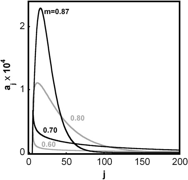
Illustrative size distributions of soluble aggregates as a function of the extent of monomer conversion, based on simulations with x = 6, δ = 1, βgn = 1000, and n* → ∞. Panels A (βcg = 0) and B (βcg = 10) correspond to simulations with Eqs 1-3 and . Panels C (β = 10-4) and D (βcg = 20) correspond to simulations with Eq. 7-10 and size dependent condensation rate coefficients (Eq. 10-14). Labels indicate the monomer mass fraction remaining for a given curve.
3.2 Parameter Estimation with the LENP model
For aggregates that remain soluble and are able to grow rapidly compared to nucleation, Eqs. 7-10 combined with Eq. 4 provide a computationally simple means to quantify separate characteristic time scales of nucleation, chain polymerization, and condensation using data regression against m(t) and simultaneously.
To assess the accuracy of τn, τg, and τc values regressed with moment equations, simulated m(t) and data over a common time range (4×t50) were generated using Eqs. 1-5 with βgn = 1000, x =6, δ =1, and κi,j ≡ 1 (κn = κw = 1), with βcg systematically increased from 0 to 10. Only data points at selected time intervals were used for regression, so as imitate typical experimental data without in situ measurements. The results below do not change substantially if a larger number and finer spacing of data points are used. The simulated data sets were nonlinearly regressed against Eqs. 7-9 and Eq. 4.
As a test of whether models that neglect condensation can reasonably fit data in which condensation is appreciable, The same simulated data were also regressed with τc → ∞; Therefore, fitting only τg and τn. Furthermore, simulated data sets from Eq. 1-5 were truncated at successively smaller extents of reaction (i.e., “early time” data only), and regression vs. Eq. 7-9 was repeated. The latter two cases help to address the question of whether {m, Mwagg} data can reliably differentiate between aggregation models that do not include condensation steps, depending on whether one uses data over multiple half lives5,16-20 or only under early-time conditions.23,28,49
Figure 6 compares The regressed time constant values (τi,fit, i = g, n, c) to the true values (τi,true, i = g, n, c) for The cases described above. The 95% confidence intervals of the fitted parameters and coefficient of determination (R2) are included in Fig. 6 to illustrate the quality of the fit in each case. The size and distribution of residuals were also examined to evaluate the quality of each fit (not shown), and were found to be consistent with the magnitude of confidence intervals and R2 values reported below. The model parameters x and δ are necessarily integers in the LENP model, and so were held constant to avoid unnecessary complications of working with mixed-integer regression. Instead, The values of x and δ were systematically varied over physically plausible ranges (x ≥ 2, δ ≥ 1) and regression of τn, τg, τc was repeated for each pair of x and δ values.
Figure 6.


Comparison of values for τg (gray), τn (white), and τc (black) obtained by regression of Eq. 7-9 against simulated experimental data from Eq. 1-3 (see text for additional details). (A) in both simulated data and fits; simulated data span four half lives. (B) same as A, but fits assumed τc → ∞ to imitate condensation free models. (C) same as B, but with simulated data sets truncated at the extent of reaction indicated by the label beside each set of bars. Error bars represent 95% confidence intervals from nonlinear least squares fits.
The best-fit results in Fig. 6 are for δ = 1, as all other δ values produced clearly inferior fits (not shown). However, fits with different values of nucleus stoichiometry (x) were not statistically distinguishable unless very large x values (> ca. 10) were used. The large-x fits were clearly inferior to the small-x fits, but it was not possible to further distinguish a best-fit x value. This is not unexpected based on previous analysis that showed reliable determination of x values required kinetic data over a relatively wide range of initial protein concentrations (C0).20 For concreteness, the results in Fig. 6 are for x = 6, the same value of x used to generate the simulated data from Eq. 1-3. More generally, this result highlights inherent difficulties in determining nucleus size from data regression vs. kinetic models when the data are available at only one or a small range of C0 values.
The results in Fig. 6A show that regression against Eq. 7-9 provides accurate parameter values for a given set of m(t) and data. This includes conditions where condensation is negligible (βcg << 1) and where it is the dominant mode of growth (βcg >> 1). In all cases, the accuracy of fitted parameters was within 5% of the true values, R2 values were greater than 0.99, and residuals were small and evenly distributed. In contrast, Fig. 6B shows that fitting with a model in which condensation is neglected clearly produced poor fits and inaccurate fitted parameter values under conditions where condensation is appreciable (βcg ~ 1) or dominant (βcg >> 1).
Figure 6C illustrates instead that if one is able to consider sufficiently early-time conditions (m ® 1), it is possible to obtain reasonably accurate values of τg and τn with a model that neglects condensation. No values of τc are shown because τc ® ∞ for the fits in Fig. 6C. The labels above each data set in Fig. 6C indicate the value of m at which the data were truncated for fitting. The truncation m value for a given data set was selected as the point at which the polydispersity first rose above a threshold value of (cf. Fig. 2D and discussion below). The results in Fig. 6C are perhaps not surprising because the initial conditions considered here are ones in which aggregates are not present, and because condensation rates are proportional to the square of the total aggregate concentration (i.e, σ2) while chain polymerization rates are linear in σ. Thus, condensation rates do not become appreciable until larger amounts of monomer have been consumed to create new aggregates. One can reach the same conclusion via an analytical perturbation solution (results not shown), such as applied previously to a condensation-free model.23 The above arguments notwithstanding, even with early-time data it is not possible to deconvolute τg and τn unless both m(t) and data are employed.
In practical terms, it is unlikely that one will know a priori whether experimental data are collected for sufficiently early times to assure condensation can be neglected. The results in Fig. 6C, when compared to those in Fig. 2D, support the empirical practice of considering condensation to be negligible if the sample polydispersity remains relatively low .4,5 The results in Fig. 2C suggest an additional criterion for neglecting condensation is that Mwagg scales linearly with (1-m). Ideally, however, it seems most prudent to instead consider models that include growth via both monomer addition and aggregate-aggregate condensation when attempting to regress accurate and mechanistically sound parameter values from experimental kinetics. An example of this approach applied to experimental data for aCgn aggregation is provided below (Sec. 3.3).
For simplicity, all preceding examples in this section used only the case of size-independent rate coefficients for condensation (κi,j = 1). From a practical standpoint, it also is often convenient to assume size-independent condensation so as to reduce the computational burden and complexity of models for regression.17,18 Furthermore, it is not clear a priori that typical experimental kinetic measurements provide sufficient information to reliably distinguish between different condensation-mediated growth mechanisms. This motivates the question, can experimental m(t) and data robustly distinguish between different models for condensation-mediated growth?
In order to address this question, Eq. 7-10 were solved with a simple diffusion-limited Smoluchowski model for κi,j (cf., Section 2) to provide simulated kinetic data that were then regressed against Eq. 7-9 with the size-independent condensation model used above. Illustrative results are shown here for simulated data (size-dependent κi,j) with βgn = 1000, βcg = 1,10,20. Figure 7A shows results for βcg = 20. The size-independent model provided excellent fits to size-dependent simulated data in all cases, with R2 > 0.99 and small, evenly distributed residuals (not shown). Despite the seemingly high quality fit for m and in Fig. 7A, the true value of increases dramatically as aggregation proceeds, although remains reasonably close to 1 throughout (data not shown). Thus, although the size-independent model fits the simulated {m, Mw} data well to within the precision of typical experimental data, the fitted value for τc is only a rough approximation to its true value.
Figure 7.

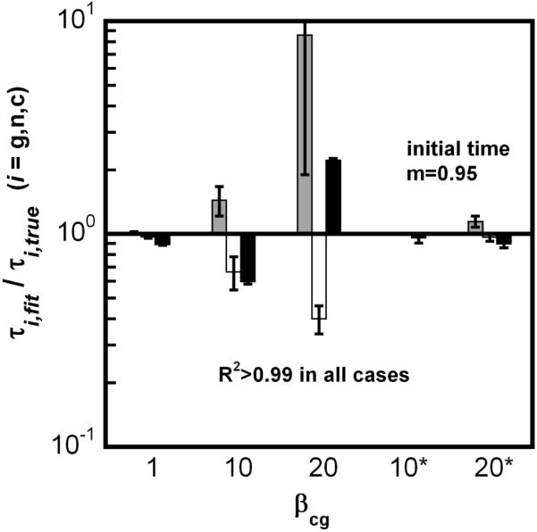
(A) Representative simulated aggregation kinetics (symbols) with size dependent condensation (Eq. 7-14, βgn = 1000, βcg = 20, x = 6, δ = 1); curves are fits to the size-independent model (Eq. 7-9, with ). (B) comparison of fitted τg (gray), τn (white), and τc (black) values from the size-independent model versus the true values, based on results analogous to panel A but for a range of βcg values. Asterisks indicate simulated data sets that were truncated at m = 0.95 before regression (see also details in text).
Fig. 7B further shows that for βcg = ca. 10 or higher, deviations are found not only in τc, but in all three fitted parameters (τg,τn,τc). Thus, although the fits appeared to be good in all test cases, the fitted values of (τg,τn,τc) were inaccurate except when condensation was not dominant over chain polymerization (βcg ~ 1 or smaller). The last two columns in Fig. 7B are for fits using a size-independent model of condensation, but with data truncated at low extents of reaction. In this case, accurate (τg,τn,τc) were obtained even when condensation is dominant (high βcg). Intuitively, this is reasonable because at low extents of reaction the aggregate size distribution will lie relatively close to the nucleus size (x), and the assumption that all ki,j values are the same as kx,x is reasonable.
The above results clearly illustrate that aggregation kinetics monitored experimentally in terms of m and Mw can qualitatively identify whether condensation steps are appreciable, but that obtaining good fits to a kinetic model will not necessarily provide fitted parameter values that accurately reflect the true values for the system. Of course, true values of model parameters cannot be known a priori for an experimental system, and so it would not be possible to statistically distinguish these mechanisms in such a situation. As a result, it cannot be generally concluded that m and Mw kinetic data on their own will be sufficient to conclusively distinguish between alternative models for aggregate condensation. Preliminary results (not shown) indicate that this limitation might be overcome if one can experimentally measure higher moments of the distribution, as well as if one can accurately quantify sample polydispersity. In practice, this may remain an outstanding challenge because these quantities are difficult if not impossible to accurately quantify with currently available commercial equipment for the typical size ranges of soluble protein aggregates (~ 1 - 102 nm). Qualitatively, however, it may be possible to distinguish between different condensation mechanisms with information regarding aggregate morphology. For example, different types of condensation mechanisms may result in aggregates with different characteristic fractal structures.51 In such cases, this argues for the importance of using additional data, such as aggregate structure or morphology, when elucidating mechanistic details of aggregation.16,51
3.3 LENP model applied to aggregation of aCgn
Figure 8 illustrates fits of the LENP model (Eq. 7-10) to experimental aggregation kinetics for α-chymotrypsinogen A (aCgn) monitored by size exclusion chromatography with inline static laser light scattering.5 The data are from two different solution conditions (summarized in the figure caption; additional details in ref. 5), and are plotted in the same format as Figures 2 and 3. In both cases the aggregates are soluble throughout the experimental time scale, and therefore n*→ ∞ for fitting with the LENP model. As was done in section 3.2, τn, τg, and τc were regressed for a range of integer values of δ and x to obtain the best least-squares fits to m(t) and data simultaneously. The best-fit values for each case, along with 95% confidence intervals are given in the caption to Figure 8.
Figure 8.

(adapted and reproduced with permission from ref. 5) Illustrative fits of the LENP model to two cases of experimental aggregation kinetics for aCgn. For both cases, the protein concentration (c0) is 1 mg mL-1 aCgn, and buffer conditions are pH 3.5, 10 mM sodium citrate buffer. The conditions differ in terms of incubation temperature and NaCl concentration: 60 °C with no NaCl (squares); 50 °C with 0.1 M NaCl (triangles). The curves are best-fits from least-squares regression vs. Eq. 7-10 with a size-independent condensation mechanism. The best-fit parameter values5 for the first data set (squares) are x = 3, δ = 1, τg = 0.1 ± 0.01 min, τn = 103 ± 102 min, and τc > 1012 min; the corresponding parameter values for the second data set (triangles) are x = 3, τg = 0.8 ± 0.1 min, τn = 500 ± 200 min, and τc = 0.1 ± 0.01 min. Panels A and B show the same data in two different formats, for easier comparion of the qualitative features from simulated data in Figures 2 and 3. The open symbols in panel A are values from light scatering; the filled symbols are the corresponding m values from chromatography. Details of the experimental protocols are given elsewhere.5
Qualitative comparison with Fig. 2 and 3 shows that the selected conditions correspond to type II (squares) and type Ia (triangles) behavior. The qualitative features for the type Ia conditions cannot be produced without including condensation steps in the model (stage V, Fig. 1): for example, the pronounced upturn of in Figure 8B, and a concomitant, large increase in polydispersity5 (results not shown here). In quantitative terms, the best fit parameter values give βgn ~ 103 in both cases. They give βcg ~ 10 and βcg << 1, respectively, for the type Ia and II cases. These results are qualitatively and quantitatively consistent with the analysis and discussion in section 3.1. Finally, the different experimental conditions for aCgn in Figure 8 correspond to aggregates with qualitatively different morphology; the aggregates for the type II conditions in Figure 8 are linear polymers,4,5 while those for the type Ia conditions are more globular and compact.5 These morphological differences are consistent with qualitative differences in growth mechanisms for limiting cases Ia and II in the LENP model. However, they do not provide sufficient information to discern additional details of the condensation mechanism (e.g., size dependent vs. size-independent ki,j). A more global search of solution conditions that give rise to behaviors other than types II and Ia for aCgn is currently underway, and will be included as part of a future report.
4. Summary
This report presents an LENP model of nonnative protein aggregation that explicitly includes the contributions of aggregate-aggregate association or condensation. The model improves upon the previous LENP model20 while maintaining its strengths and ability to capture a wide variety of experimental behaviors. The global behavior and application to simulated data are illustrated primarily using a size-independent condensation mechanism similar to that employed previously,17,18 and to a lesser extent using a simple Smoluchowski, diffusion-limited condensation mechanism. Illustrative examples are also included via application of the LENP model to experimental aggregation kinetics of α-chymotrypsinogen A.5
The results illustrate a number of ways to qualitatively determine whether soluble aggregate growth occurs via chain polymerization, aggregate-aggregate condensation, or a combination of both. It is shown that this assessment is easily done by measuring both monomer loss (or mass percent conversion to aggregate) and weight-average molecular weight when monitoring aggregation kinetics. When high molecular weight aggregates remain soluble, moment-based kinetic equations provide a means to quantitatively separate the time scales or inverse rate coefficients for nucleation (τn), growth by chain polymerimation (τg), and condensation (τc). This requires time dependent data on aggregate molecular weight Mw, and cannot be done with only data for monomer concentration m. However, even regression against both m and Mw is not necessarily sufficient to distinguish between alternative models for condensation. Use of early time data to provide accurate values of τn and τg was also evaluated and found to provide reasonable estimates even when details of a condensation mechanism are unknown. The current LENP model is also easily adaptable to include more complex aggregate growth mechanisms.
Acknowledgements
Financial support from Merck & Co. (YL) and the National Institutes of Health (CJR; grant no. R01 EB006006) is gratefully acknowledged.
5. Appendix
The dynamic material balances of monomer (m), nuclei (ax) and larger aggregates (ai,i>x) for the reaction scheme in Fig. 1 are given by Eq. A1-A3, assuming each step in Fig. 1 is an elementary reaction obeying mass-action kinetics, and stages 1 and 2 are pre-equilibrated. Rate coefficients and equilibrium constants are defined in Fig. 1 and are consistent with more detailed descriptions given in ref. 20.
| (A1) |
| (A2) |
| (A3) |
Eqs. A1-3 are similar to expressions that were derived previously20 except that terms are included to account for the consumption of nuclei by condensation steps, as well as formation and consumption of other aggregates through condensation. Symbols in the above equations are explained in Section 2.1, and are consistent with previous work.20 The corresponding moment equations follow by taking weighted sums over dai/dt from i = x to ∞, along with the model parameters defined in Sec. 2: Zeroth Moment:
| (A4) |
First Moment:
| (A5) |
Second Moment:
| (A6) |
Eq. A4 and A6 are approximate only in that they neglect the terms and respectively. These terms are due to the self association reaction ai + ai → ai+i where two same-sized aggregates are consumed, and are negligible when the aggregate size distribution is not close to monodisperse, as is the case when nucleation is slow compared to growth via chain or condensation polymerization.
References
- (1).Fink AL. Folding & Design. 1998;3:R9. doi: 10.1016/S1359-0278(98)00002-9. [DOI] [PubMed] [Google Scholar]
- (2).Roberts CJ. Biotechnology and Bioengineering. 2007;98:927. doi: 10.1002/bit.21627. [DOI] [PubMed] [Google Scholar]
- (3).Chi EY, Krishnan S, Randolph TW, Carpenter JF. Pharmaceutical Research. 2003;20:1325. doi: 10.1023/a:1025771421906. [DOI] [PubMed] [Google Scholar]
- (4).Weiss WF, IV, Hodgdon TK, Kaler EW, Lenhoff AM, Roberts CJ. Biophys J. 2007;93:4392. doi: 10.1529/biophysj.107.112102. [DOI] [PMC free article] [PubMed] [Google Scholar]
- (5).Li Y, Weiss WF, IV, Roberts CJ. J Pharm Sci. Submitted. [Google Scholar]
- (6).Weiss WF, IV, Young TM, Roberts CJ. J Pharm Sci. 2008 doi: 10.1002/jps.21521. [DOI] [PubMed] [Google Scholar]
- (7).Cromwell MEM, Hilario E, Jacobson F. AAPS Journal. 2006;8:E572. doi: 10.1208/aapsj080366. [DOI] [PMC free article] [PubMed] [Google Scholar]
- (8).Wang W. International Journal of Pharmaceutics. 2005;289:1. doi: 10.1016/j.ijpharm.2004.11.014. [DOI] [PubMed] [Google Scholar]
- (9).Dobson CM. Seminars in Cell & Developmental Biology. 2004;15:3. doi: 10.1016/j.semcdb.2003.12.008. [DOI] [PubMed] [Google Scholar]
- (10).Uversky VN, Fink AL. Biochimica et Biophysica Acta, Proteins and Proteomics. 2004;1698:131. [Google Scholar]
- (11).Rosenberg AS. AAPS Journal. 2006;8:E501. doi: 10.1208/aapsj080359. [DOI] [PMC free article] [PubMed] [Google Scholar]
- (12).Purohit VS, Middaugh CR, Balasubramanian SV. J Pharm Sci. 2006;95:358. doi: 10.1002/jps.20529. [DOI] [PMC free article] [PubMed] [Google Scholar]
- (13).Philo JS. Aaps J. 2006;8:E564. doi: 10.1208/aapsj080365. [DOI] [PMC free article] [PubMed] [Google Scholar]
- (14).Goetz H, Kuschel M, Wulff T, Sauber C, Miller C, Fisher S, Woodward C. J Biochem Biophys Methods. 2004;60:281. doi: 10.1016/j.jbbm.2004.01.007. [DOI] [PubMed] [Google Scholar]
- (15).Andrews JM, Roberts CJ. Biochemistry. 2007;46:7558. doi: 10.1021/bi700296f. [DOI] [PubMed] [Google Scholar]
- (16).Pallitto MM, Murphy RM. Biophys J. 2001;81:1805. doi: 10.1016/S0006-3495(01)75831-6. [DOI] [PMC free article] [PubMed] [Google Scholar]
- (17).Modler AJ, Gast K, Lutsch G, Damaschun G. J Mol Biol. 2003;325:135. doi: 10.1016/s0022-2836(02)01175-0. [DOI] [PubMed] [Google Scholar]
- (18).Speed MA, King J, Wang DIC. Biotechnology And Bioengineering. 1997;54:333. doi: 10.1002/(SICI)1097-0290(19970520)54:4<333::AID-BIT6>3.0.CO;2-L. [DOI] [PubMed] [Google Scholar]
- (19).Andrews JM, Weiss WF, IV, Roberts CJ. Biochemistry. 2008;47:2397. doi: 10.1021/bi7019244. [DOI] [PubMed] [Google Scholar]
- (20).Andrews JM, Roberts CJ. J Phys Chem B. 2007;111:7897. doi: 10.1021/jp070212j. [DOI] [PubMed] [Google Scholar]
- (21).Roberts CJ. Journal of Physical Chemistry B. 2003;107:1194. [Google Scholar]
- (22).Roberts CJ. Non Native Protein Aggregation: Pathways, Kinetics, and Shelf Life Prediction. In: Murphy RM, Tsai AM, editors. Misbehaving Proteins: Protein Misfolding, Aggregation, and Stability. Springer; New York: 2006. p. 17. [Google Scholar]
- (23).Ferrone F. Methods in Enzymology. 1999;309:256. doi: 10.1016/s0076-6879(99)09019-9. [DOI] [PubMed] [Google Scholar]
- (24).Oosawa F, Asakura S. Thermodynamics of the Polymerization of Proteins. Academic Press; London: 1975. [Google Scholar]
- (25).Mahler HC, Friess W, Grauschopf U, Kiese S. J Pharm Sci. 2008 doi: 10.1002/jps.21566. [DOI] [PubMed] [Google Scholar]
- (26).Ramkrishna D. Population Balances: Theory and Applications to Particulate Systems in Engineering. 1st edition Academic Press; New York: 2007. [Google Scholar]
- (27).Lee CC, Nayak A, Sethuraman A, Belfort G, McRae GJ. Biophys J. 2007;92:3448. doi: 10.1529/biophysj.106.098608. [DOI] [PMC free article] [PubMed] [Google Scholar]
- (28).Chen SM, Ferrone FA, Wetzel R. Proceedings Of The National Academy Of Sciences Of The United States Of America. 2002;99:11884. doi: 10.1073/pnas.182276099. [DOI] [PMC free article] [PubMed] [Google Scholar]
- (29).Powers ET, Powers DL. Biophys J. 2006;91:122. doi: 10.1529/biophysj.105.073767. [DOI] [PMC free article] [PubMed] [Google Scholar]
- (30).Chi EY, Krishnan S, Kendrick BS, Chang BS, Carpenter JF, Randolph TW. Protein Science. 2003;12:903. doi: 10.1110/ps.0235703. [DOI] [PMC free article] [PubMed] [Google Scholar]
- (31).Gibson TJ, Murphy RM. Biochemistry. 2005;44:8898. doi: 10.1021/bi050225s. [DOI] [PubMed] [Google Scholar]
- (32).Kim JR, Gibson TJ, Murphy RM. Biotechnol Prog. 2006;22:605. doi: 10.1021/bp050407d. [DOI] [PubMed] [Google Scholar]
- (33).Chi EY, Kendrick BS, Carpenter JF, Randolph TW. J Pharm Sci. 2005;94:2735. doi: 10.1002/jps.20488. [DOI] [PubMed] [Google Scholar]
- (34).Kurganov BI. Biochemistry (Mosc) 1998;63:364. [PubMed] [Google Scholar]
- (35).Liu J, Andya JD, Shire SJ. AAPS Journal. 2006;8:E580. doi: 10.1208/aapsj080367. [DOI] [PMC free article] [PubMed] [Google Scholar]
- (36).Bourhim M, Kruzel M, Srikrishnan T, Nicotera T. J Neurosci Methods. 2007;160:264. doi: 10.1016/j.jneumeth.2006.09.013. [DOI] [PubMed] [Google Scholar]
- (37).LeVine H., 3rd Protein Sci. 1993;2:404. doi: 10.1002/pro.5560020312. [DOI] [PMC free article] [PubMed] [Google Scholar]
- (38).Kendrick BS, Cleland JL, Lam X, Nguyen T, Randolph TW, Manning MC, Carpenter JF. J Pharm Sci. 1998;87:1069. doi: 10.1021/js9801384. [DOI] [PubMed] [Google Scholar]
- (39).Webb JN, Webb SD, Cleland JL, Carpenter JF, Randolph TW. Proc Natl Acad Sci U S A. 2001;98:7259. doi: 10.1073/pnas.131194798. [DOI] [PMC free article] [PubMed] [Google Scholar]
- (40).Hiemenz PC. Polymer Chemistry: The Basic Concepts. Marcel Dekker; New York: 1984. [Google Scholar]
- (41).Wen J, Arakawa T, Philo JS. Anal Biochem. 1996;240:155. doi: 10.1006/abio.1996.0345. [DOI] [PubMed] [Google Scholar]
- (42).Roberts CJ, Darrington RT, Whitley MB. J Pharm Sci. 2003;92:1095. doi: 10.1002/jps.10377. [DOI] [PubMed] [Google Scholar]
- (43).Barzykin AV, Shushin AI. Biophysical Journal. 2001;80:2062. doi: 10.1016/S0006-3495(01)76180-2. [DOI] [PMC free article] [PubMed] [Google Scholar]
- (44).Smoluchowski M. v. Z. Phys. Chem. 1917;92:129. [Google Scholar]
- (45).Sandkühler P. AIChE Journal. 2003;49:1542. [Google Scholar]
- (46).Hilbe JM. Negative Binomial Regression. Cambridge University Press; Cambridge, UK: 2007. [Google Scholar]
- (47).Walpole RE. Probability & Statistics for Engineers & Scientists. 8th ed. Pearson, Prentice Hall; Upper saddle River, NJ: 2006. [Google Scholar]
- (48).Tsai AM, van Zanten JH, Betenbaugh MJ. Biotechnol Bioeng. 1998;59:273. [PubMed] [Google Scholar]
- (49).Ignatova Z, Gierasch LM. Biochemistry. 2005;44:7266. doi: 10.1021/bi047404e. [DOI] [PubMed] [Google Scholar]
- (50).Buswell AM, Middelberg APJ. Biotechnology And Bioengineering. 2003;83:567. doi: 10.1002/bit.10705. [DOI] [PubMed] [Google Scholar]
- (51).Meakin P. Annual Review of Physical Chemistry. 1988;39:237. doi: 10.1146/annurev.pc.39.100188.000245. [DOI] [PubMed] [Google Scholar]