Analyzing Information Flow in Brain Networks with Nonparametric Granger Causality

Abstract

Multielectrode neurophysiological recording and high-resolution neuroimaging generate multivariate data that are the basis for understanding the patterns of neural interactions. How to extract directions of information flow in brain networks from these data remains a key challenge. Research over the last few years has identified Granger causality as a statistically principled technique to furnish this capability. The estimation of Granger causality currently requires autoregressive modeling of neural data. Here, we propose a nonparametric approach based on widely used Fourier and wavelet transforms to estimate Granger causality, eliminating the need of explicit autoregressive data modeling. We demonstrate the effectiveness of this approach by applying it to synthetic data generated by network models with known connectivity and to local field potentials recorded from monkeys performing a sensorimotor task.

Introduction

Multivariate neural recordings are becoming commonplace. Such recordings promise to offer unparalleled insights into how different brain areas work together to achieve thought and behavior, and how such coordinated brain activity breaks down in disease. While the accumulation of data from all signal modalities, including electroencephalography (EEG), magnetoencephalography (MEG), functional magnetic resonance imaging (fMRI) and positron emission tomography (PET), continues at an astonishing rate, how to effectively analyze these data to extract understandings of brain functions presents a key challenge. Analytically, cross correlations and ordinary coherence spectra have remained the main measures for assessing statistical interdependence and functional connectivity among the participating areas of a brain network. These measures, however, have not played a significant role in providing reliable information on effective connectivity (Friston, 1994) which is primarily concerned with the directions of neural interactions and how one neural system exerts influence over another. Structural equation modeling (SEM) has been used for this purpose in fMRI and PET. SEM theoretically hypothesizes the directions of interactions among the set of measured variables and quantifies the interaction strength via correlation analysis. The shortcoming of SEM is that it depends critically on a preexisting theoretical framework.

Granger causality (Granger, 1969; Geweke, 1982) has emerged in recent years as a leading technique for inferring directions of neural interactions and information flow directly from data. The basic idea can be traced back to Wiener who is the first to recognize the importance of temporal ordering in the inference of causal relations (Wiener, 1956). Granger formalized Wiener’s idea in terms of autoregressive (AR) models of time series (Granger, 1969) and the technique now bears his name. Consider two simultaneously acquired time series. If the autoregressive prediction of the first time series at present time could be improved by including the past information of the second time series we say that the second time series has a causal influence on the first. The role of the two time series can be reversed to address the causal influence in the opposite direction. This pairwise time domain approach was later generalized in two important directions. First, the spectral decomposition of Granger’s time domain causality was proposed by Geweke in 1982 (Geweke, 1982). The resultant Granger causality spectra are important for the analysis of EEG and MEG data as these data are rich in oscillatory content. Second, for a system with more than two simultaneously acquired time series, conditional Granger causality, both in the time domain and in the frequency domain (Granger, 1980; Geweke, 1984), were developed for distinguishing direct from indirect causal influences. Recent work has demonstrated that this measure plays an indispensable role in linking neural network dynamics with the underlying neural network anatomy (Chen et al., 2006; Ding et al., 2006). Neuroscience applications of Granger causality have begun to appear with increasing frequency in recent years (Bernasconi and Konig, 1999; Liang et al., 2000; Brovelli et al., 2004; Hesse et al., 2003; Kaminski et al., 2001; Harrison et al., 2003; Goebel et al., 2003; Sato et al., 2006; Chen et al., 2006), revealing insights not possible with traditional methods such as cross correlation and ordinary coherence.

Autoregressive modeling, the basis of the current parametric Granger causality techniques, has proven effective for data modeled by low-order AR processes. However, AR methods sometimes fail to capture complex spectral features in data that require higher order AR models (Mitra and Pesaran, 1999). Additionally, the proper determination of model order remains a concern, although this concern may be mitigated by the recently proposed Bayesian framework (Harrison et al., 2003). Widely used Fourier and wavelet-transform based nonparametric spectral methods have the advantage of fewer assumptions and are free from the aforementioned shortcomings (Mitra and Pesaran, 1999; Percival and Walden, 1993). But, presently, these nonparametric methods are mainly used for spectral power and coherence, and do not have the capability for estimating Granger causality.

In this paper we propose a nonparametric approach to Granger causality analysis. Combining spectral density matrix factorization with Geweke’s time series decomposition, the new approach estimates both pairwise and conditional Granger causality directly from Fourier and wavelet transforms, bypassing the step of parametric data modeling. We validate the new approach by applying it first to simulated data generated by networks with known connectivity and temporal dynamics, and then to local field potential data from monkeys performing a sensorimotor task. It is expected that, by basing the estimation of Granger causality on simple and widely used data transformations, the nonparametric approach will provide an alternative to the parametric approach, enabling a wider practice of effective connectivity analysis, and eventually become a significant addition to the repertoire of analytical tools for multivariate neural data processing.

Materials and Methods

In multivariate spectral analysis, the key quantity is the spectral matrix from which one derives measures such as power, coherence, multiple coherence and partial coherence. There are two ways to arrive at the spectral matrix: parametric and nonparametric. In the parametric approach, autoregressive models are fit to the data. One obtains the spectral matrix from the model transfer function and the noise covariance matrix which are also used in the spectral formulation of Granger causality. In the nonparametric approach, one obtains the spectral matrix directly from Fourier or wavelet transforms of data. The spectral matrix needs to be factorized to yield the transfer function and the noise covariance matrix. This step is the basis for the nonparametric Granger causality method proposed in this work.

Experiment

The experiment was conducted in the Laboratory of Neuropsychology at the National Institute of Mental Health during 1984–1988 and animal care was in accordance with the institutional guidelines at that time. The monkey initiated each trial by pressing a lever with its hand and keeping it pressed. After a random interval (uniformly distributed between 120 and 2200 ms) from the time the lever was pressed, a visual stimulus, either for a GO response (to release the lever) or for a NO-GO response (to continue holding the lever), was presented for 100 ms and the monkey made the required response within 500 ms from the stimulus onset. Local field potential data were acquired at a sampling rate of 200 Hz simultaneously from up to 15 distributed cortical sites of one hemisphere in two macaque monkeys (right hemisphere for subject GE and left hemisphere for subject LU) using transcortical bipolar electrodes. The recording took place over many sessions with each session comprising around 1000 trials (for further experimental details, see Bressler et al., 1993; Brovelli et al., 2004; Ledberg et al., 2007). For the ensemble of trials selected for this work, the ensemble mean time series from each record site was subtracted from the individual single-trial time series to ensure that the resulting data could be treated as coming from a zero-mean stochastic process (Ding et al., 2006). Physiologically, the data recorded from −90ms to 500 ms could be considered as reflecting several distinct cognitive states. From −90 ms to 35 ms (0 ms being the stimulus onset) the monkey held the lever steady while attending the screen and anticipating the imminent onset of visuomotor processing. The visual information presented at 0 ms arrived at various recording sites between 50 to 100 ms. The monkeys made GO or NOGO decisions before 200 ms (Ledberg et al., 2007). The average reaction time for a correct go response was around 270 ms (Ledberg et al., 2007).

Multitaper Spectral Estimation

The multitaper spectral and cross-spectral method introduced by Thompson (Thompson, 1982) is known to provide smooth spectral density function estimates (Percival and Walden, 1993; Percival and Walden, 2000;Mitra and Pesaran, 2001). It involves the utilization of the discrete prolate spheroidal sequences (DPSS) (Slepian and Pollak, 1961) known as tapers. To obtain average spectral and cross-spectral estimates, the time series from each trial is multiplied by a pre-selected number of orthogonal tapers, the products are Fourier-transformed, and the resulting transforms are cross-multiplied and averaged over individual tapers. Multiple realizations or trials (experimental repetitions) further give rise to an ensemble over which the expectation (averaging) is taken. Specifically, consider simultaneously acquired multiple time series: {x_rt}(r=1,…, p; t=1,…, n), where r is the channel index and t is the discrete time index. Then, for a single trial, the multi-taper cross-spectrum estimator between channels l and m at frequency f is

$$S_{lm}(f)=\frac{\mathrm{\Delta }}{K}\sum _{k=1}^K\left\{\sum _{s=1}^n{w}_s(k)x_{ls}{e}^{-i2\pi fs\mathrm{\Delta }}\right\}\left\{\sum _{t=1}^n{w}_t(k)x_{mt}{e}^{i2\pi ft\mathrm{\Delta }}\right\},$$ (1)

where w(k) (k = 1, 2,…, K) are K orthogonal tapers of length n and Δ is the sampling interval. For l = m we obtain the auto-spectrum. The spectral density matrix $S(f)=\left(\begin{array}{ccc}{S}_{11}(f)& \dots & S_{1p}(f)\\ \dots & \dots & \dots \\ S_{p1}(f)& \dots & S_{pp}(f)\end{array}\right)$ is obtained by averaging the cross-spectrum estimators for all pairs of channels over individual trials. The diagonal terms of this matrix S(f) represent auto-spectra whereas the off-diagonal terms cross-spectra.

Wavelet Spectral Estimation

The wavelet transform provides time-frequency representation of a signal and is useful to analyze time-varying (nonstationary) processes (Daubechies, 1990; 1992; Percival and Walden, 2000). Convolution of a given signal x(t) with a scaled and translated version of a prototype wavelet function ψ(η), which satisfies zero-mean ( $\underset{-\infty }{\overset{\infty }{\int }}d\eta \psi (\eta )=0$) and unity square-norm ( $\underset{-\infty }{\overset{\infty }{\int }}d\eta \mid \psi (\eta ){\mid }^2=1$) conditions, results in the continuous wavelet transform at time t and scale s:

$$W(t,s)=\frac{1}{\sqrt{s}}\underset{-\infty }{\overset{\infty }{\int }}d\eta {\psi }^{\ast }\left(\frac{\eta -t}{s}\right)x(\eta ),$$ (2)

where (*) indicates the complex conjugate. Scale s is related with frequency f. By varying s and translating along time t, one can construct a form of time-frequency representation of the signal. In this work, we chose a complex Morlet wavelet, consisting of a plane wave modulated by a Gaussian: ψ(η)=π^−1/4e^iωη e^−η2/2, as the prototype wavelet with ω ≥ 6 (Torrence and Compo, 1998). The Gaussian envelope e^−η2/2 localizes the wavelet in time and ω determines time/scale resolution. Higher values of ω provide better scale or frequency resolution but poorer time resolution. The wavelet cross spectrum between the signals recorded at channels l and m at time t and scale s is then

$$W{S}_{lm}(t,s)=\langle W{x}_l(t,s)W^{\ast }{x}_m(t,s)\rangle ,$$ (3)

where the expectation (denoted by < >) is taken over all the trials recorded. Setting l = m, one obtains auto-wavelet spectra. The full wavelet spectral matrix WS(t, s) is computed by using all pairs of channels. Using the relationship between Fourier frequency f and wavelet scale s for the prototype wavelet used (see Torrence and Compo, 1998 for the complex Morlet wavelet), we obtained the full wavelet spectral matrix WS(t, f) at time t and frequency f.

Spectral Matrix Factorization

Spectral matrix factorization is a procedure for constructing a sequence of unique generating functions (or minimum-phase spectral factors) out of spectral density matrices (Sayed and Kailath, 2001). It was introduced by Wiener in 1949 (Wiener, 1949) for a single time series and was later extended to multiple time series by Wiener and Masani in 1957 (Wiener and Masani, 1957) and Youla in 1961 (Youla, 1961). Since then, it has found extensive applications in the analysis and design of linear systems. It has been applied in the fields of digital signal processing (Anderson and Moore, 1979), control theory (Balakrishnan and Boyd, 1992), communications (Fischer, 2005), geophysics (Fomel and Claerbout, 2003), and helioseismology (Rickett and Claerbout, 2000).

The spectral density matrix, such as Fourier transform-based S(f) or wavelet transform-based WS(t_i, s) at any time point t_i that satisfies $\underset{-\pi }{\overset{\pi }{\int }}logdet(S(f))df>-\infty$, can be factored into a set of unique minimum-phase functions:

$$\text{S}=\mathrm{\Psi }{\mathrm{\Psi }}^{\ast },$$ (5)

where Ψ is the minimum-phase, spectral density matrix (left) factor which has a Fourier series expansion in nonnegative powers of e^i2πf: $\mathrm{\Psi }={\displaystyle \sum _{k=0}^{\infty }}{A}_k{e}^{ik2\pi f}$, and Ψ* is its complex conjugate transpose. There are several algorithms available for spectral matrix factorization (see, for review, Sayed and Kailath, 2001). For this work, we implemented Wilson’s algorithm (Wilson, 1972), which is noted for its superb numerical efficiency (Goodman et al., 1997). A convergence theorem for an iterative method used in this algorithm guarantees the existence of factorization of rational spectral density matrices (Wilson, 1978).

From the minimum-phase spectral factor Ψ, noise covariance matrix Σ and minimum-phase transfer function H(f) can be obtained as

$$\mathrm{\sum }=A_0{A_0}^T$$ (6)

and

$$H=\mathrm{\Psi }{A_0}^{-1}$$ (7)

such that ΨΨ^*=HΣH^*. Here, T stands for matrix transposition. As indicated earlier, spectral matrix factorization is thus a key step in the estimation of Granger causality as it provides the quantities H and Σ that are readily available from the parametric data modeling but not so from the traditional nonparametric spectral analysis.

Granger Causality Measures

The measures of Granger causality are based on the notion that the causal (driving) variable can help forecast the effect (driven) variable (Granger, 1969; Geweke, 1982). The reduction in the unexplained variance of the effect variable (say X: x₁, x₂,…, x_n) as a result of inclusion of the causal variable (say Y: y₁, y₂,…, y_n) in linear autoregressive modeling ( $x_n={\displaystyle \sum _{k=1}^{\infty }}{a}_k{x}_{n-k}+{\epsilon }_n;x_n={\displaystyle \sum _{k=1}^{\infty }}{b}_k{x}_{n-k}+{\displaystyle \sum _{k=1}^{\infty }}{c}_k{y}_{n-k}+{\eta }_n$), that is, $\frac{{\mathrm{\sum }}_2}{{\mathrm{\sum }}_1}=\frac{var({\eta }_n)}{var({\epsilon }_n)}<1$, marks the existence of a causal influence from Y to X in time domain. In the frequency domain, the total spectral power (auto-spectrum) of the effect variable (X) is decomposed into its intrinsic power and the causal contribution from Y and the ratio of the total power to the intrinsic power indicates the presence of causal influence (Geweke, 1982; see Ding et al., 2006 for a review).

Pairwise Granger causality

In the time domain, $F_{Y\to X}=ln\frac{{\mathrm{\sum }}_1}{{\mathrm{\sum }}_2}$, where Σ₁ is X’s unexplained variance in its autoregression, whereas Σ₂ is X’s unexplained variance in the joint (X and Y) regression. In the frequency domain, $I_{Y\to X}(f)=ln\frac{S_{xx}(f)}{{\stackrel{\sim }{S}}_{xx}(f)}$, where S_xx (f) is the total power and S̃_xx (f) is the intrinsic power. Using S(f)= H (f) ΣH^*(f), where the transfer function H(f) and the noise covariance matrix Σ are derived either from spectral matrix factorization (nonparametric approach) or AR data modeling (parametric approach, the causality from Y to X at frequency f becomes:

$$I_{Y\to X}(f)=ln\frac{S_{xx}(f)}{S_{xx}(f)-({\mathrm{\sum }}_{yy}-{{\mathrm{\sum }}_{xy}}^2/{\mathrm{\sum }}_{xx})\mid H_{xy}(f){\mid }^2},$$ (8)

where the term in the denominator is the total power minus the causal contribution representing the intrinsic power.

Conditional Granger causality

In a system of three or more time series, it is often desirable to find out whether a causal influence between any pair of time series is direct or mediated by others, which cannot be identified by the bivariate (or pairwise) measure of causality. An example of this scenario is illustrated in Figure 1, where Y exerts a causal influence on X only via Z. A pairwise analysis will reveal a nonzero causality from Y to X (dashed arrow). This is clearly an incorrect inference and was called a ‘prima facia cause’ (causality on its first appearance) by Granger (Granger, 1980). To resolve such ambiguity has led to the development of conditional Granger causality (Granger, 1980; Geweke, 1984). In the time domain, the Granger causality from Y to X conditional on Z is defined as: $F_{Y\to X\mid Z}=ln\frac{{\mathrm{\sum }}_{xx}(X,Z)}{{\mathrm{\sum }}_{xx}(X,Y,Z)}$, where Σ_xx (X, Z) is the variance of the noise in the joint regression of X and Z, and Σ_xx (X, Y, Z) the variance in the regression of X, Y and Z, both variances being associated with X variable. In the frequency domain,

Figure 1. Three-node network model system.

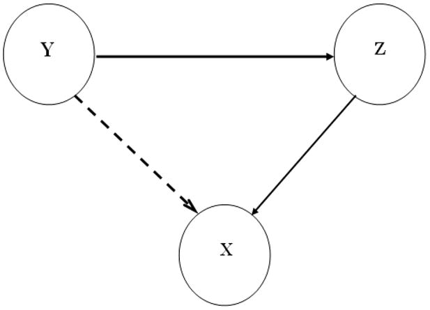
X, Y, and Z are stationary stochastic processes interacting with each other in a network. Y has a causal influence on Z and Z, in turn, has a causal influence on X (represented by solid arrows). Y has an indirect influence on X via Z, as shown by a dashed arrow. Direct and indirect directional influences can be distinguished by the conditional Granger causality.

$$I_{Y\to X\mid Z}(f)=ln\frac{{\mathrm{\sum }}_{xx}(X,Z)}{\mid Q_{xx}(f){\widehat{\mathrm{\sum }}}_{xx}(X,Y,Z)Q_{xx}{(f)}^{\ast }\mid },$$ (9)

where the quantities in the denominator inside the logarithm are functions of the transfer function and the noise covariance matrix (see Ding et al., 2006).

Mathematically, the spectral measures are related to the time-domain measures through:

$$F_{Y\to X}=\frac{2}{f_s}\underset{0}{\overset{f_s/2}{\int }}{I}_{Y\to X}(f)df$$ (10)

and

$$F_{Y\to X\mid Z}=\frac{2}{f_s}\underset{0}{\overset{f_s/2}{\int }}{I}_{Y\to X\mid Z}(f)df,$$ (11)

where f_s is the data sampling rate.

Using the nonparametric approach, one can first compute I_Y→X (f) and I_Y→X|Z (f) at all frequencies and perform the required integration to obtain the corresponding time domain quantities.

Results

The nonparametric approach for estimating Granger causality consists of the following steps: (i) construct spectral density matrix S from Fourier transforms or wavelet transforms of multi-channel time series data, (ii) factorize spectral density matrix: S = ΨΨ* where Ψ is the minimum-phase spectral factor, (iii) derive noise covariance matrix Σ and transfer function H from Ψ according to Eqs. (6) and (7), and (iv) use S, H, Σ in Geweke’s formulae (Geweke, 1982; 1984) to arrive at Granger causality spectra. The time domain Granger causality can be obtained by integrating the spectral representation over frequency. In our implementation of the above steps, the multi-taper method (Mitra and Pesaran, 1999) is used to construct the spectral density matrix in the Fourier transform-based approach and the Morlet wavelet (Morlet et al., 1982; Torrence and Compo, 1998) is used in the wavelet transform-based approach. Spectral density matrix factorization is achieved by Wilson’s algorithm (Wilson, 1972; 1978).

Below, we first demonstrate the excellent performance of the nonparametric Granger causality techniques on simulated data generated from stationary and non-stationary network models where the interaction patterns are known. We then apply the techniques to local field potentials recorded from monkeys performing a sensorimotor task for which a Granger causality analysis has been published in the past with the parametric approach (Brovelli et al., 2004; Chen et al., 2006; Ding et al., 2006). We stress that both the parametric and the nonparametric approaches produce consistent findings that are physiologically interpretable and yield new insights not possible with other methods.

The simulation models

Two models are considered for generating simulated time series. The first model is a 3-node network where X, Y, and Z are jointly stationary stochastic processes described by the following autoregressive (AR) process: X(t) = 0.8 X(t−1) −0.5 X(t−2) + 0.4*Z(t−1)+ η (t), Y(t) = 0.53 Y(t−1) −0.8 Y(t−2) + ξ(t) and Z(t) = 0.5 Z(t−1) − 0.2 Z(t−2) + 0.5 Y(t−1) + ε(t). Here t is a discrete time index, η (t), ξ(t) and ε(t) are independent white noise processes with zero means and non-zero variances. As illustrated by the solid arrows in Fig. 1, Y has a causal influence on Z, and Z, in turn, drives X. The dashed arrow implies that Y has an indirect influence on X which is mediated by Z. The pairwise approach cannot distinguish direct from indirect causal effects; the conditional Granger causality is required for unequivocal resolution. The second model is a two-node network with nonstationary dynamics: Y1(t) = 0.53 Y1(t−1) −0.8 Y1(t−2) + ε₁(t) Y2(t−1)+ ξ(t) and Y2(t) = 0.53 Y2(t−1) −0.8 Y2(t−2) + ε₂(t) Y1(t−1)+ η (t), where ε₁(t) and ε₂(t) are time-varying coupling strengths.

Analysis of simulated time series

Fourier transform-based methods

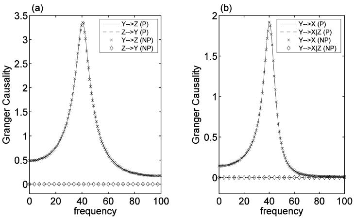
For the first 3-node network model, letting var(η) = 0.25, var(ξ) = 1 and var(ε) = 0.25, we obtained a dataset of 4000 trials (i.e. realizations) with each trial consisting of 4000 data points. The discrete time steps are assumed to be equivalent to a sampling rate of 200 Hz. Figure 2(a) shows a comparison between the parametric (P) and nonparametric (NP) calculations of pairwise Granger causality between Y and Z. It is clearly seen that both approaches yield identical results, recovering the correct network connectivity pattern of unidirectional Y→ Z driving. Since the data set consists of many realizations of long time series, the parametric analysis results can be considered as the theoretical results (Ding et al. 2000). Figure 2(b) shows that there is significant pairwise Granger causal influence from Y to X, but the conditional Granger causality measure Y→ X|Z (causal influence from Y to X conditional on Z) confirmed that the causal influence from Y to X was completely mediated by Z, since Y→ X|Z was zero at all frequencies. This is again consistent with the design of the model network. Expected results were also found for other combinations of variables.

Figure 2. Comparison between Fourier-based nonparametric and parametric measures of Granger causality.

(a) spectra of pairwise causality between Y and Z, and (b) spectra of causality from Y to X, both pairwise and conditional on Z. The parametric (P) and nonparametric (NP) measures demonstrate excellent agreement.

Wavelet transform-based methods

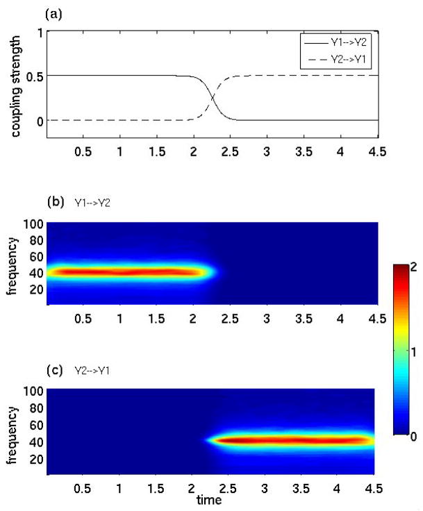
The simulated data above were also subjected to the wavelet transform-based pairwise and conditional Granger causality analysis. Results identical to that in Figure 2 were obtained (not shown), demonstrating that wavelet-based methods are fully capable of uncovering network connectivity from multiple stationary time series. Their ability to reveal temporal patterns of causal influences was tested by simulating the second 2-node nonstationary network model consisting of interacting variables Y1 and Y2. Letting variances be 0.25 and letting the coupling strengths ε₁(t) and ε₂(t) vary according to the profiles given in Figure 3(a), we obtained 1000 trials of data with each trial containing 900 points. From the model design we see that Y1 drives Y2 (Y1→Y2) in the first half of the simulation time interval, Y2 drives Y1 (Y2→Y1) in the second half, and the slow transitions between the two modes of causal influences occur during 1.5 < t < 3 sec. As shown in Figure 3(b) and 3(c) , the wavelet-based Granger causality technique clearly recovers these predicted patterns with high temporal precision.

Figure 3. Wavelet-based Granger causality: a means for studying time-varying causal influences.

The first panel shows the time course of coupling strengths in the model system consisting of Y1 and Y2 interacting with each other. In the first half of the simulated time interval, Y1 exerts causal influence on Y2, and, in the second half, it is the opposite. The slow transitions between the two driving modes have been modeled by the tangent of hyperbolic functions in the time-interval t = 1.5 to 3 sec. The coupling reversal occurs at t = 2.25. The second and third panels of time-frequency Granger causality maps show that the wavelet-based Granger causality technique is able to recover the temporal dynamics of the causal influences.

Application to experimental data

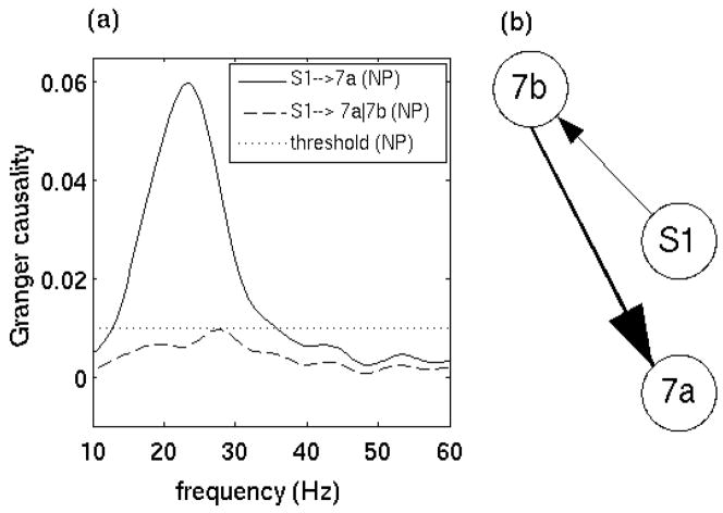
Local field potentials (LFPs) were sampled at a rate of 200 Hz from up to 15 distributed sites of one hemisphere in two macaque monkeys (right hemisphere in monkey GE and left hemisphere in monkey LU) performing a GO/NOGO visual pattern discrimination task. The sites chosen for analysis are located in the sensorimotor cortex, including primary somatosensory area (S1), primary motor area (M1), posterior parietal areas 7a and 7b for monkey GE, and S1, M1, and 7b for monkey LU. Our focus here is network activity during the prestimulus stage when the monkey maintained steady pressure on a depressed hand lever and anticipated the imminent onset of visuomotor processing. Parametric power, coherence, and Granger causality analysis of these data (Brovelli et al., 2004; Chen et al., 2006; Ding et al., 2006) has reported the following findings: (i) synchronized beta-frequency (15–30 Hz) oscillations linked together diverse sensorimotor areas to form a large-scale cortical network, (ii) strong Granger causal influences (information) flowed from S1 to M1 and to 7a and 7b, (iii) 7b exerted further Granger causal influences on M1, and (iv) Granger causal influences from the motor cortex into the post-central areas were small and statistically insignificant. The causal influence from S1 to 7a was further subjected to a conditional Granger causality analysis as anatomical considerations suggested that such influence could be mediated by area 7b and this was found to be indeed the case.

The above results led to the hypothesis that the beta oscillation network in the sensorimotor cortex facilitates the maintenance of steady pressure on the depressed hand lever. The directionality provided by Granger causality is consistent with the known functional roles of the involved cortical areas, and has played an instrumental role in the formulation of this hypothesis. To further test this hypothesis, Zhang et al. (2005) studied the temporal evolution of the beta oscillation network, employing a moving window parametric analysis. For GO trials, as the monkey prepared and carried out the lever-releasing hand movement following stimulus presentation, the need for pressure maintenance was removed and the beta oscillation as well as the causal influences underlying the oscillation network vanished as a result. Below we test the nonparametric Granger causality techniques on the same data with the goal of validating these new techniques in the context of the previous parametric findings and a well-established interpretational framework.

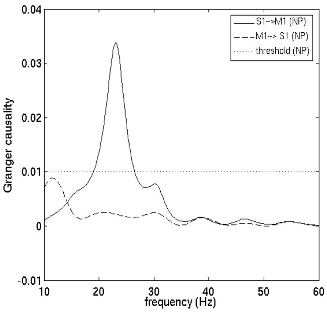
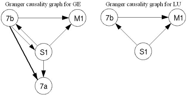
All pairwise combinations were first analyzed for each monkey subject in the prestimulus time period (−90 to 35 ms) by the Fourier-based methods. Figure 4 shows the Granger causality spectra for one such pair, M1 and S1, in GE. A random permutation approach (Blair and Karniski, 1993; Brovelli et al., 2004), which involved creating 1000 permutations of the local field potential dataset by random shuffling of the trial order independently for each site, was used to find thresholds for statistical significance. Significant S1→ M1 (solid) causal influence is seen in the beta frequency range (~22 Hz) while M1→ S1 (dotted) is below significance threshold. Figure 5 summarizes the pairwise analysis by displaying the Granger causality graphs for the beta oscillation network in both monkey subjects. These graphs are identical to the ones obtained by the parametric techniques reported in (Ding et al., 2006). The causal influence from S1 to 7a is further analyzed with the conditional Granger causality and the result is shown in Fig. 6. While pairwise S1→7a is statistically significant, the conditional causality S1→ 7a|7b (dashed lines) are below the corresponding significance thresholds (dotted lines), suggesting that the causal influence from S1 to 7a is most likely mediated by 7b. Figure 6(c) shows a refined Granger causality graph involving S1, 7b and 7a. This graph is identical to the one obtained by the parametric method and can be interpreted in terms of the known anatomical pathways linking these areas (Felleman and van Essen, 1991; Ding et al. 2006). The wavelet-based methods are also considered for the same data. The results are qualitatively the same as those shown in Figs. 4–6. We next performed a time-frequency Granger causality analysis based on wavelet transforms for the entire GO trial. The result revealed that the causal influence from S1 to M1 in the beta frequency range disappeared during movement preparation and execution (Fig 7). This is in agreement with the parametric results reported by Zhang et al. (2005).

Figure 4. Fourier-based pairwise Granger causality spectra for experimental data.

nonparametric measures of Granger causality between primary somatosensory (S1) and primary motor (M1) areas. There is a significant causal influence from S1 to M1 at about 22 Hz, which falls within the beta frequency range (14–30 Hz). The significance thresholds (shown by dotted lines) have been numerically obtained under a null hypothesis of no interdependence at a level p < 10⁻⁶.

Figure 5. Granger causality graphs in the beta frequency range for monkeys GE and LU obtained by the Fourier-based non-parametric approach.

These significant pairwise connectivity patterns are identical to the ones obtained by the parametric technique.

Figure 6. Fourier-based pairwise and conditional Granger causality spectra for the network of areas S1, 7a and 7b.

(a) pairwise spectrum for S1→7a (solid line) and conditional Granger causality spectra S1→7a|7b (dashed line) and (b) revised Granger causality network based on direct causal influences.

Figure 7. Wavelet-based time-frequency analysis of Granger causality for GO trials.

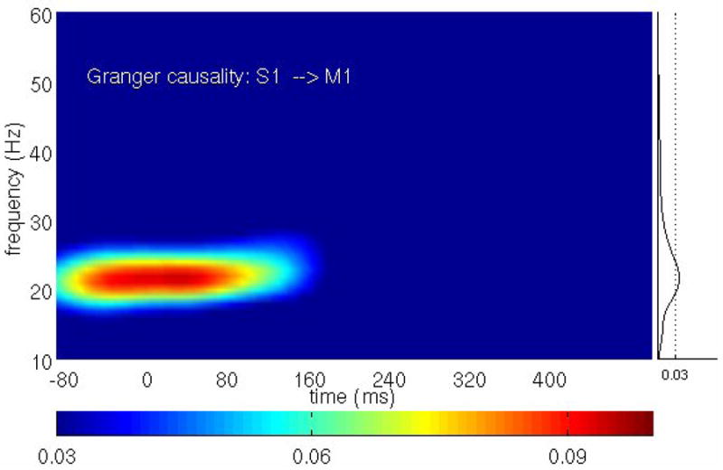
The causal influence from S1 to M1 in the GO condition disappeared during movement preparation and execution, supporting the hypothesis that the beta oscillations exist to facilitate motor maintenance behavior. The plot on the right side shows the average causal influence over time (solid curve) and the significance threshold at p < 10⁻⁶ (dotted line) computed from the time period −90 to 35 ms.

Discussion

Granger causality, structural equation modeling (SEM) (McIntosh and Gonzalez-Lima, 1994), and the recently proposed dynamic causal modeling (DCM) (Friston et al., 2003; Lee, et al., 2006) are the main statistical methods for effective connectivity analysis. Other techniques, including phase-dynamics approach (Rosenblum and Pikvosky, 2001) and transfer entropy (Schreiber, 2000; Lungrella and Sporns, 2006), have also been attempted for the same purpose. SEM and DCM rely on the existence of a neural theoretical framework and are often limited by the lack of precise anatomical and physiological constraints. Since Granger causality is a more data-driven method, it has witnessed rapid growth in recent years in applications to neurophysiological and neuroimaging data. To date, parametric modeling remains the basis for Granger causality inference in the frequency domain. While nonparametric Granger causality tests have appeared in the past they are all formulated in the time domain (Bell et al., 1996; Diks and Panchenko, 2006; Hiemstra and Jones, 1994). As the parametric spectral approach requires the autoregressive models of data, concerns have been raised regarding the strong underlying assumptions and its suitability for data with complex power spectral content (Mitra and Pesaran, 1999; see Figure 1 in the Supplementary Material). In this paper, we propose a nonparametric spectral approach in which Granger causality is estimated directly from Fourier and wavelet transforms of data, removing the need for autoregressive models. The mathematical basis of our method is a combination of spectral matrix factorization and Geweke’s spectral formulation of Granger causality. Although there are other spectral measures for inferring causal influences, including directed transfer function (DTF) (Kamiski and Blinowska, 1991; Kaminski et al., 2001), partial directed coherence (PDC) (Bacala and Sameshima, 2001), and directed DTF (Korzeniewska, et al. 2003), Geweke’s measure is expressed in terms of variance explained and is thus more statistically interpretable.

The new nonparametric approach was tested on simulated data. Two examples were considered. In the first example, multiple realizations of time series were generated by a 3-node network model. The pattern of network connectivity was correctly recovered by both the Fourier- and wavelet-based methods. The second example simulated a nonstationary process in a 2-node network model. The wavelet-based methods were able to resolve the fine temporal dynamics by capturing the rapid reversal of causal influences built into the model. The nonparametric approach was further tested on recordings of local field potentials from monkeys performing a sensorimotor task. The previously reported causal network dynamics in the beta frequency range obtained with the parametric techniques (Brovelli et al., 2004; Chen et al., 2006; Ding et al., 2006) were reproduced by both the Fourier- and wavelet-based methods. This provides a validation for the new approach. Although, unlike simulations, the true answer in an experimental situation is not a priori known, a strong support for such an assertion is that the information flow patterns reported before are both physiologically and anatomically interpretable, and have led to a testable hypothesis regarding the function of the beta oscillation network in the sensorimotor cortex. In addition to electrophysiological signals, we also applied the proposed nonparametric approach to fMRI time series obtained in a complex rhythmic finger-tapping task (Dhamala et al., 2003; see Figure S2 in the Supplementary Material). There, the causal influence pattern was found to be in agreement with the direction of information flow postulated in the movement control literature.

Evaluating causal relations from multivariate neural data is an important problem and is attracting increasing research interest. An important caveat that is applicable to any technique in the area of multivariate data analysis concerns the issue of hidden variables. For two measured variables, if their relationship is caused by a third variable that is not observed, the analysis result will be ambiguous. This is a distinct possibility in systems as complex as the brain and cannot be easily remedied. This hidden variable problem impacts not only Granger causality analysis but also every other multivariate statistic used in neuroscience today. In this regard, well thought-out experiments combined with strategic placements of electrodes hold the key to avoid ambiguous analysis interpretations.

Although the nonparametric approach removes the need for extracting AR models from data, it has its own initial choices of parameters, including the number of tapers, wavelet prototype and the time-frequency resolution trade-off (ω for the Morlet wavelet). The number of tapers determines the amount of smoothing necessary to reduce the variance of the spectral estimates. The results included in this article were obtained by using 3 tapers. We varied the number of tapers up to 12 and found that the results were not very sensitive to the number of tapers used. However, at a very high number, the spectral peak gets distorted, e.g., a single peak splits into two. The general guideline is that the number of tapers should be chosen to reduce the variance while not overly distorting the spectrum (see Mitra and Pesaran, 1999). For the wavelet applications, we used the complex Morlet wavelet with ω ≥ 6 in the form proposed by Torrence and Compo (Torrence and Compo, 1998), where the higher ω ensures a good frequency resolution at the cost of time resolution. This choice of wavelet is for convenience and our wavelet-based techniques can be implemented for any wavelet base. The test of the nonparametric Granger causality techniques are performed on simulated datasets with a large number of long trials. These methods can also be used reliably with fewer trials. An increased number of trials contribute to a smaller variance in the spectral estimates. A single, sufficiently long stationary time series can be segmented into smaller epochs, each of which can be regarded as an individual trial. The use of multitaper techniques can further reduce estimation bias in case of a dataset with shorter length. However, when there is too little data (short length and few trials), both parametric and nonparametric estimates may not be reliable.

The foregoing discussion suggests that the proposed nonparametric approach provides an alternative way for estimating Granger causality that complements rather than replaces the parametric approach. In the parametric methods, the model order parameter is often selected based on standard criteria such as the Akaike information criterion (Akaike, 1974) or the Bayesian information criterion (Schwarz, 1978). In case these criteria are not effective due to finite data length or other reasons, one can choose the model order which gives the best possible match between the parametric and nonparametric power spectra. In addition, it is known that for short time series, nonparametric spectral methods produce biased estimates. (A systematic study of how data length influences Fourier-based Granger causality estimation is presented in the appendix.) In this case the parametric methods hold a distinct advantage when multiple realizations (trials) of the same process are available (Ding et al., 2000). However, for reasonably long time series, which are usually available in most electrophysiological or imaging experiments, the proposed nonparametric Granger causality techniques are robust and yield excellent results.

Appendix

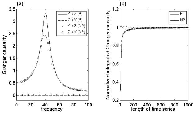
In a typical cognitive neuroscience experiment, the brain undergoes rapid state change, from anticipation to sensation to decision-making to movement execution, all within a few hundreds milliseconds. This dynamical process can be captured on a fine time scale by performing spectral analysis with short moving windows. When data of multiple trials are treated as coming from the same underlying stochastic process the AR model based parametric approach yields reliable spectral estimates for power and coherence within each short window. For very short time series, spectral estimates with Fourier based nonparametric approach are biased (Ding et al., 2000). To determine the reliability and asymptotic behaviors of the proposed Granger causality methods, we compared nonparametric and parametric estimates using simulated time series data of various trial lengths while keeping the number of trials fixed. The data came from the Y and Z channels of the 3-node network model (Figure 1). Figure 8(a) shows nonparametric and parametric pairwise Granger causality spectra when each trial is 70 time points long. Figure 8(b) is the time-domain Granger causality by integrating parametric and nonparametric spectra as a function of trial length. The number of trials for all cases was 4000. As indicated earlier, parametric spectral estimates from a large number of trials are known to approach true theoretical values [Ding et al., 2000], which is the basis for these comparisons. From Figure 8(a) it is clear that even for relatively short segments of data, besides a slight underestimate of the peak value, the nonparametric technique can recover the correct direction (Y→Z) and peak location (40 Hz) of causal influences. The nonparametric estimate rapidly approaches the parametric or true value as the data length is increased (Fig 8(b)).

Figure 8. Effect of data length.

(a) nonparametric and parametric pairwise Granger causality spectra and (b) integrated parametric and nonparametric Granger causality as a function of data length. Even for a short segment of data, nonparametric measure provides the correct direction of causal influences. The nonparametric estimate can rapidly approach the true value as the data length is increased.

References

- Akaike H. A new look at the statistical model identification. IEEE Trans Automat Cont. 1974;19:716–723. [Google Scholar]
- Anderson B, Moore JB. Optimal Filtering. Prentice-Hall; New Jersey: 1979. [Google Scholar]
- Bacala LA, Sameshima K. Partial directed coherence: A new concept in neural structure determination. Biol Cybern. 2001;84:463–474. doi: 10.1007/PL00007990. [DOI] [PubMed] [Google Scholar]
- Balakrishnan V, Boyd S. Global optimization in control system analysis and design. In: Leondes CT, editor. Control and Dynamic Systems: Advances in Theory and Applications. Vol. 53. Academic Press; New York, New York: 1992. pp. 1–55. [Google Scholar]
- Bell D, Kay J, Malley J. A non-parametric approach to non-linear causality testing. Economics Letters. 1996;51:7–18. [Google Scholar]
- Bernasconi C, Konig P. On the directionality of cortical interactions studied by structural analysis of electrophysiological recordings. Biol Cybern. 1999;81:199–210. doi: 10.1007/s004220050556. [DOI] [PubMed] [Google Scholar]
- Blair RC, Karniski W. An alternative method for significance testing of waveform difference potentials. Psychophysiology. 1993;30:518–524. doi: 10.1111/j.1469-8986.1993.tb02075.x. [DOI] [PubMed] [Google Scholar]
- Bressler SL, Coppola R, Nakamura R. Episodic multiregional cortical coherence at multiple frequencies during visual task performance. Nature. 1993;366:153–156. doi: 10.1038/366153a0. [DOI] [PubMed] [Google Scholar]
- Brovelli A, Ding M, Ledberg A, Chen Y, Nakamura R, Bressler SL. Beta oscillations in a large-scale sensorimotor cortical network: directional influences revealed by Granger causality. Proc Natl Acad Sci USA. 2004;101:9849–9854. doi: 10.1073/pnas.0308538101. [DOI] [PMC free article] [PubMed] [Google Scholar]
- Chen Y, Bressler SL, Ding M. Frequency decomposition of conditional Granger causality and application to multivariate neural field potential data. J Neurosci Methods. 2006;150:228–237. doi: 10.1016/j.jneumeth.2005.06.011. [DOI] [PubMed] [Google Scholar]
- Daubechies I. Ten Lectures on Wavelets, Society for Industrial and Applied Mathematics 1992 [Google Scholar]
- Daubechies I. The wavelet transform time-frequency localization and signal analysis. IEEE Trans Inform Theory. 1990;36:961–1004. [Google Scholar]
- Dhamala, et al. Neural correlates of the complex rhythmic finger tapping. NeuroImage. 2003;20:918–926. doi: 10.1016/S1053-8119(03)00304-5. [DOI] [PubMed] [Google Scholar]
- Diks C, Panchenko V. A new statistic and practical guidelines for nonparametric Granger causality testing. Journal of Economic Dynamics and Control. 2006;30 (9–10):1647–1669. [Google Scholar]
- Ding M, Bressler SL, Yang W, Liang H. Short-window spectral analysis of cortical event-related potentials by adaptive multivariate autoregressive modeling: data preprocessing, model validation, and variability assessment. Biological Cybernetics. 2000;83:35–45. doi: 10.1007/s004229900137. [DOI] [PubMed] [Google Scholar]
- Ding M, Chen Y, Bressler S. Granger causality: Basic theory and application to neuroscience. In: Schelter B, Winterhalder B, Timmer MJ, editors. Handbook of Time Series Analysis: Recent Theoretical Developments and Applications. Wiley-VCH; Berlin: 2006. pp. 437–459. [Google Scholar]
- Felleman DJ, Van Essen. D. C. Distributed hierarchical processing in the primate cerebral cortex. Cerebral Cortex. 1991;1:1–47. doi: 10.1093/cercor/1.1.1-a. [DOI] [PubMed] [Google Scholar]
- Fischer R. Sorted Spectral Factorization of Matrix Polynomials in MIMO Commincations. IEEE Trans Comm. 2005;53:945–951. [Google Scholar]
- Fomel S, Claerbout J. Multidimensional recursive filter preconditioning in geophysical estimation problems. Geophysics. 2003;68:577–588. [Google Scholar]
- Friston KJ. Functional and effective connectivity in neuroimaging: a synthesis. Hum Brain Mapp. 1994;2:56–78. [Google Scholar]
- Friston KJ, Harrison L, Penny W. Dynamic causal modeling. NeuroImage. 2003;19:1273–1302. doi: 10.1016/s1053-8119(03)00202-7. [DOI] [PubMed] [Google Scholar]
- Granger CWJ. Investigating Causal Relations by Economic Models and Cross-Spectral Methods. Econometrica. 1969;37:424–438. [Google Scholar]
- Granger CWJ. Testing for causality: a personal viewpoint. J Econ Dyn Control. 1980;2:329–352. [Google Scholar]
- Geweke J. Measurement of linear-dependence and feedback between multiple time-series. J Amer Statist Assoc. 1982;77:304–313. [Google Scholar]
- Geweke J. Measures of conditional linear-dependence and feedback between time-series. J Amer Statist Assoc. 1984;79:907–915. [Google Scholar]
- Goebel R, Roebroeck A, Kim DS, Formisano E. Investigating directed cortical interactions in time-resolved fMRI data using vector autoregressive modeling and Granger causality mapping. Magn Reson Imaging. 2003;21:1251–61. doi: 10.1016/j.mri.2003.08.026. [DOI] [PubMed] [Google Scholar]
- Goodman TNT, Micchelli CA, Rodrigues G, Seatzu S. Spectral factorization of Laurent polynomials. Adv Comput Math. 1997;7:429–454. [Google Scholar]
- Hiemstra C, Jones JD. Testing for linear and nonlinear Granger causality in the stock price-volume relation. Journal of Finance. 1994;49:1639–1664. [Google Scholar]
- Harrison L, Penny WD, Friston KJ. Multivariate autoregressive modeling of fMRI time series. Neuroimage. 2003;19:1477–1491. doi: 10.1016/s1053-8119(03)00160-5. [DOI] [PubMed] [Google Scholar]
- Hesse W, Moller E, Arnold M, Schack B. The use of time-variant EEG Granger causality for inspecting directed interdependencies of neural assemblies. J Neurosci Methods. 2003;124:27–44. doi: 10.1016/s0165-0270(02)00366-7. [DOI] [PubMed] [Google Scholar]
- Kamiski MJ, Blinowska KJ. A new method of the description of the information flow in the brain structures by a modified directed transfer function (dDTF) method. J Neurosci Methods. 1991;125:195–207. doi: 10.1016/s0165-0270(03)00052-9. [DOI] [PubMed] [Google Scholar]
- Kaminski MJ, Ding M, Truccolo WA, Bressler SL. Evaluating causal relations in neural systems: Granger causality, directed transfer function and statistical assessment of significance. Biol Cybern. 2001;84:463–474. doi: 10.1007/s004220000235. [DOI] [PubMed] [Google Scholar]
- Korzeniewska A, Kasicki S, Kaminski M, Blinowska KJ, Kasicki S. Determination of information flow direction among brain structures by a modified directed transfer function (dDTF) method. J Neurosci Methods. 2003;125:195–207. doi: 10.1016/s0165-0270(03)00052-9. [DOI] [PubMed] [Google Scholar]
- Ledberg A, Bressler SL, Ding M, Coppola R, Nakamura R. Large-scale visuomotor integration in the cerebral cortex. Cereb Cortex. 2007;17:44–62. doi: 10.1093/cercor/bhj123. [DOI] [PubMed] [Google Scholar]
- Lee L, Friston K, Horwitz B. Large-scale neural models and dynamic causal modeling. NeuroImage. 2006;30:1243–1254. doi: 10.1016/j.neuroimage.2005.11.007. [DOI] [PubMed] [Google Scholar]
- Liang H, Ding M, Nakamura R, Bressler SL. Causal Influences in Primate Cerebral Cortex during Visual Pattern Discrimination. NeuroReport. 2000;11:2875–2880. doi: 10.1097/00001756-200009110-00009. [DOI] [PubMed] [Google Scholar]
- Lungarella M, Sporns O. Mapping information flow in sensorimotor networks. PLoS Comp Biol. 2006;2:1301–1312. doi: 10.1371/journal.pcbi.0020144. [DOI] [PMC free article] [PubMed] [Google Scholar]
- McIntosh AR, Gonzalez-Lima F. Structural equation modeling and its application to network analysis in functional brain imaging. Hum Brain Map. 1994;2:2–22. [Google Scholar]
- Mitra PP, Pesaran B. Analysis of dynamic brain imaging data. Biophys J. 1999;76:691–708. doi: 10.1016/S0006-3495(99)77236-X. [DOI] [PMC free article] [PubMed] [Google Scholar]
- Morlet J, Arens G, Fourgeau E, Giard D. Wave propagation and sampling theory-Part I & II: Complex signal and scattering in multilayered media. Geophysics. 1982;47:203–236. [Google Scholar]
- Percival D, Walden A. Wavelet Methods for Time Series Analysis. Cambridge Univ. Press; Cambridge, UK: 2000. [Google Scholar]
- Percival D, Walden A. Spectral Analysis for Physical Applications: Multitaper and Conventional Univariate Techniques. Cambridge University Press; Cambridge, UK: 1993. [Google Scholar]
- Rickett JE, Claerbout JF. Calculation of the Sun’s acoustic impulse response by multidimensional spectral factorization. Solar Physics. 2000;192:203–210. [Google Scholar]
- Rosenblum MG, Pikovsky AS. Detecting direction of coupling in interacting oscillators. Phys Rev E. 2001;64:045202–4. doi: 10.1103/PhysRevE.64.045202. [DOI] [PubMed] [Google Scholar]
- Sato JR, Junior EA, Takahashi DY, de Maria FM, Brammer MJ, Morettin PA. A method to produce evolving functional connectivity maps during the course of an fMRI experiment using wavelet-based time-varying Granger causality. Neuroimage. 2006;31:187–96. doi: 10.1016/j.neuroimage.2005.11.039. [DOI] [PubMed] [Google Scholar]
- Sayed H, Kaylath T. A survey of spectral factorization methods. Numer Linear Algebra Appl. 2001;8:467–496. [Google Scholar]
- Schreiber T. Measuring information transfer. Phys Rev Lett. 2000;85:461–464. doi: 10.1103/PhysRevLett.85.461. [DOI] [PubMed] [Google Scholar]
- Schwarz G. Estimating the dimension of a model. Ann Statist. 1978;4:461–464. [Google Scholar]
- Thomson DJ. Spectrum estimation and harmonic analysis. Proc IEEE. 1982;70:1055–1096. [Google Scholar]
- Slepian D, Pollak HO. Prolate spheroidal wavefunctions Fourier analysis and uncertainty. I Bell Sys Tech J. 1961;40:43–63. [Google Scholar]
- Torrence C, Compo G. A practical guide to wavelet analysis. Bull Amer Meteor Soc. 1998;79:61–78. [Google Scholar]
- Wiener N. The theory of prediction. In: Beckenbach EF, editor. Modern Mathematics for the Engineer. McGraw-Hill; New York: 1956. [Google Scholar]
- Wiener N. Extrapolation, Interpolation and Smoothing of Stationary Time Series with Engineering Applications. Wiley; New York: 1949. [Google Scholar]
- Wiener N, Masani P. The prediction theory of multivariate stochastic processes, I. Acta Math. 1957;98:111–150. [Google Scholar]; II. Acta Math. 99:93–137. [Google Scholar]
- Wilson GT. The factorization of matricial spectral densities. SIAM J Appl Math. 1972;23:420–426. [Google Scholar]
- Wilson GT. A convergence theorem for spectral factorization. J Multivariate Analysis. 1978;8:222–232. [Google Scholar]
- Walden AT. A unified view of multitaper multivariate spectral estimation. Biometrika. 2000;87:767–788. [Google Scholar]
- Youla DC. On the factorization of rational matrices. IRE Trans Information Theory IT. 1961;7:172–189. [Google Scholar]
- Zhang Y, Bressler SL, Chen Y, Nakamura R, Ding M. Beta and gamma synchronization and desynchronization in monkeys during a visual discrimination task. Soc Neurosc Abstr. 2005;31 Prog. No. 413.18. [Google Scholar]
Associated Data
This section collects any data citations, data availability statements, or supplementary materials included in this article.