

Abstract
Background and Aims
The strong influence of environment and functioning on plant organogenesis has been well documented by botanists but is poorly reproduced in most functional–structural models. In this context, a model of interactions is proposed between plant organogenesis and plant functional mechanisms.
Methods
The GreenLab model derived from AMAP models was used. Organogenetic rules give the plant architecture, which defines an interconnected network of organs. The plant is considered as a collection of interacting ‘sinks’ that compete for the allocation of photosynthates coming from ‘sources’. A single variable characteristic of the balance between sources and sinks during plant growth controls different events in plant development, such as the number of branches or the fruit load.
Key Results
Variations in the environmental parameters related to light and density induce changes in plant morphogenesis. Architecture appears as the dynamic result of this balance, and plant plasticity expresses itself very simply at different levels: appearance of branches and reiteration, number of organs, fructification and adaptation of ecophysiological characteristics.
Conclusions
The modelling framework serves as a tool for theoretical botany to explore the emergence of specific morphological and architectural patterns and can help to understand plant phenotypic plasticity and its strategy in response to environmental changes.
Key words: Trophic plasticity, plant growth, functional–structural models, dynamic system, interactions, GreenLab
INTRODUCTION
The recent history of plant growth modelling and simulation is notable for its diversity. Since the 1990s, a new type of model has emerged, commonly called functional–structural models (Sievänen et al., 2000). Generally speaking, the architectural development of the plant provides the sources, according to which photosynthesis is determined, and the compartments, among which the biomass produced is distributed. The representation of the plant 3-D architecture gives a structure to reproduce fluxes of biomass or hormones (Prusinkiewicz et al., 2007) as well as exchanges with the environment (Evers et al., 2005). This approach aims at understanding ‘the complex interactions between the plant architecture and the physical and biological processes that drive the plant development’ (Godin and Sinoquet, 2005).
In most functional–structural models, a descriptive architecture is used as a basis for plant functioning and feedback of this functioning on plant morphogenesis is generally reduced to the morphological features of organs, especially their sizes. In their review, Le Roux et al. (2001) consider that the description of interactions between tree structure and function is the weakest point of most tree growth models, whereas the strong influence of environment and functioning on plant organogenesis has been extensively reported by botanists (Barthélémy and Caraglio, 2007). Most plants only partially express their growth potential according to growth conditions. Sultan (2000) wrote ‘Only recently has plasticity been widely recognized as a significant mode of phenotypic diversity and hence as an important aspect of how organisms develop, function and evolve in their environments’.
The first model with feedback between organogenesis and photosynthesis was described by Borchert and Honda (1984): an apex initiates a lateral branch if an incoming flux of substances exceeds a given threshold value. This idea was used in Prusinkiewicz et al. (1997) to simulate different branching structures according to a theoretical flux. However, these first attempts were not linked to a real photosynthetic model. Geometrical responses to the environmental conditions of growth were also introduced by Blaise and de Reffye (1994) and Mech and Prusinkiewicz (1996). In their approaches, plant form is not controlled by functioning but by exogenous mechanisms (spatial competition, for example). In some functional–structural models, the physiological mechanisms control not only the size of organs but also their number, thus inducing a phenotypic plasticity during plant growth.
For example, the SIMWAL model has random bud burst, with a probability that depends on growth unit volume, axis order, bud position and growth unit reserves (Balandier et al., 2000). Likewise, in the LIGNUM model, the number of branches depends on the size of the mother growth unit (Perttunen et al., 1998). In the functional–structural tree model ALMIS, the effects of structural and functional factors interact during tree growth (Eschenbach, 2005) and the development of the tree structure has different characteristics (numbers and arrangements of organs, self-thinning) according to the variations in environmental factors.
In this context, the purpose of our work is to propose a model of interactions between functional mechanisms and development. We particularly focus on the various expressions of plasticity related to trophic competition, in keeping with the most recent knowledge in plant architecture. It is important to keep in mind that plant carbon balance is not the only driving force for plasticity. There are some phenomena that we will not be able to model, such as the tillering in rice induced by hormonal signals (Buck-Sorlin et al., 2008). However, this article aims at exploring to what extent trophic determinisms can account for the high variability of plant phenotypic plasticity, the modelling of which is a great challenge (Fourcaud et al., 2008).
We use the GreenLab model (de Reffye and Hu, 2003; Yan et al., 2004), which is the mathematical framework derived from AMAP models (de Reffye et al., 1997). Organogenetic rules give the plant structure, which can be defined as an interconnected network of organs. Source–sink relationships among these organs determine biomass production and allocation. A consistent time unit for architectural development and ecophysiological functioning is defined. It allows the discrete dynamic system of growth to be derived, and its state variables are sufficient to deduce the whole-plant architecture (cf. Mathieu et al., 2006). The model is not devoted to a specific species but aims at modelling any kind of plant, even though some of them are out of reach for the moment.
In this study, we present an upgraded version of the model in which the feedback between functioning and architecture is controlled by a single variable representative of the source–sink balance during plant growth: the ratio of available biomass to demand. This choice is coherent with several observations that will be detailed later in this article. For example, it is linked to the size of buds, which has a significant impact on future shoot development (Sabatier and Barthélémy, 2001) and to the sizes of growth units that control the appearance of lateral axes (Nicolini and Chanson, 1999).
In Mathieu et al. (2008), we showed how rhythms were automatically generated by the model for some parameter values. In this paper, we present a generalization of this model to reproduce the alterations in plant development as a consequence of the dynamic changes in the ratio of biomass to demand along plant growth. We focus on a theoretical definition of the model, but some applications of the model gave satisfactory results when it was confronted with real experimental data: see Mathieu et al. (2007) for a model of fruit abortion as a function of the source–sink ratio or Letort et al. (2008) for a model of the beech tree branching system.
In this paper, we first introduce the dynamic system of growth based on plant organogenesis that is used as the mathematical framework of modelling. The basic principles of the ecophysiological submodels used to compute plant functioning are reprised. Then we detail how the ratio of available biomass to the total organ demand can be used as the key variable to control the main aspects of plant organogenesis. Finally, we introduce a method for model calibration and discuss the limitations of our approach.
MATERIALS AND METHODS
Discretization of the growth process
Botanists generally agree on the fact that plants are modular organisms that develop by the repetition of elementary botanical entities or constructional units (Bell, 1991; de Kroon et al., 2005). The most elementary of these entities is the phytomer, which is composed of one internode, the node (i.e. insertion points of leaves on a stem) located at its tip and the corresponding one or several leaves and associated lateral buds (White, 1979). It may also bear a flower or fruit.
Plant growth is discretized with a time step called the growth cycle (GC) that is based on the rhythm of organ appearance. Its definition depends on the form of growth: rhythmic or continuous. Plants have a rhythmic growth when the shoots have marked endogenous periodicity and cessation of extension (Hallé and Martin, 1968). Then, the growth unit is the portion of axis that develops during an uninterrupted period of shoot extension (Barthélémy and Caraglio, 2007) and a growth cycle starts with the appearance of a new growth unit. In contrast, when shoots have no marked endogenous cessation of extension, the growth is said to be continuous (Hallé et al., 1978) and the growth cycle is based on the phyllochron (Rickman and Klepper, 1995). In both cases, we will consider plant architecture as constant during the whole time step and the chronological age of a plant is defined as the number of growth cycles it has existed for.
At each growth cycle, biomass production and allocation to organs are deduced from plant structure and are computed with empirical equations describing source–sink relationships. Since the GreenLab model is well described in the literature (see Cournède et al., 2006, or de Reffye et al., 2008 for the latest versions), in the following of this section we focus on the parts of the model dealing with interactions between growth and development. However, the equations for the whole model are given in the Appendix and Table 1 gives a description of the variables and parameters.
Table 1.
Abbreviations for variables and parameters
| Notation | Description |
|---|---|
| GC | Growth cycle |
| PB, FB | Potential buds, active buds |
| Pm | Number of different physiological ages |
| t | Chronological age of the plant (in GC) |
| k, l | Indices for the physiological age |
| Q(t) | Biomass produced at cycle t (g) |
| D(t) | Plant demand at cycle t |
| DPB(t), DFB(t) | Demand of the potential buds, demand of the active buds |
| DE(t) | Demand of the organs in expansion |
| DC(t) | Demand of the cambium (plant secondary growth) |
| pO(n) | Sink of an organ O of chronological age n. O is replaced by A for blades, P for peduncles, F for fruit |
| pR(t) | Sink strength of the root system at cycle t |
| pB,k | Sink strength of a bud of physiological age k |
| QPB(t) | Biomass allocated to the future organs |
| S(t) | Total plant leaf surface area (m2) |
| EPAR(t) | Variable proportional to the photosynthetically active radiation (MJ m−2) |
| μ | Radiation use efficiency (g MJ−1) |
| κ | Extinction coefficient of the Beer–Lambert law |
| Sp | Parameter characteristic of the stand density; 1/Sp is correlated with the stand density (m2) |
| sk | Bud of physiological age k |
| Uk(t,n) | Growth unit of physiological age k and chronological age n at cycle t |
| mkl(t,n) | Phytomer of chronological age n at cycle t on a bearing axis of physiological age k and with an axillary bud of physiological age l |
| mO,kl | Number of organs of type O on a phytomer mkl(t,n). O is replaced by A for blades, P for peduncles, F for fruit, PB for potential buds |
| vk(t,n) | Number of growth units of physiological age k, chronological age n at cycle t |
| ukl(t) | Number of phytomers described by mkl(t,1) |
| bkl(t) | Number of buds that become active at the end of cycle t |
| uF,k(t) | Number of fruits in a growth unit of physiological age k at cycle t |
| τk(n) | Life span of a branch of physiological age k born at cycle n |
| qB,k(t) | Amount of biomass allocated to a bud sk at growth cycle t |
| Parameters of the affine functions, modelling the retroaction of growth on development | |
| αkl, α′kl | Number of active buds of physiological age l born by phytomers of physiological age k |
| βkl, β′kl | Number of phytomers of physiological age k with buds of physiological age l |
| γk, γ′k, | Life span of branches of physiological age k |
| δk, δ′k | Number of fruits in growth units of physiological age k |
GreenLab model of organogenesis
The architecture of a plant can be seen as a hierarchical branching system in which axes can be grouped into categories defined by a combination of morphological, anatomical or functional parameters (Barthélémy et al., 1997). An axis is here defined as a rectilinear stem composed of a succession of phytomers or growth units. The different categories of axes are characterized by the notion of physiological age. Pm denotes the number of different physiological ages for a given plant.
Plant organogenesis will be obtained by the arrangement of the different kinds of phytomers. The categorization of axes by the notion of physiological age allows a structural factorization of the plant, and we use a formal grammar to describe the plant structure (cf. de Reffye et al., 2003; Cournède et al., 2006). Each phytomer is represented by a letter: mkl(t,n) denotes a phytomer of chronological age n at cycle t and physiological age k bearing lateral axes of physiological age 1 and sl denotes a bud of physiological age l, with l ∈ {k, … Pm}. Unbranched phytomers are represented by •. At cycle t, a new growth unit of physiological age k is formed by ukl(t) phytomers mkl(t,1). The composition of the growth unit Uk(t,n) of physiological age k and chronological age n as a set of phytomers and lateral buds is given in eqn (1) and illustrated in Fig. 1. It is described by the concatenation of the phytomers that compose the growth unit. The concatenation operator is represented by the multiplicative sign.
 |
1 |
Fig. 1.

Illustration of growth units. (A) The youngest growth units of the trunk in an acroton plant (Abies sp.), indicated by the white line (from Barthélémy and Caraglio, 2007). The topological arrangement of lateral branches along the parent axis may be associated with an increasing gradient in length and/or vigour of the branches. (B) Schematic representation of the composition of such growth units, with the notations used in eqn (1). The variables upl(t) and bpl(t) indicate, respectively, the numbers of phytomers of type mpl(t,1) (physiological age p with buds of physiological age l, chronological age 1 at cycle t) and lateral branches born by these phytomers, with l ∈ {p, … , Pm}. Each physiological age is represented by a different colour. The white arrow stands for the growth from cycle 1 to cycle 2.
The number of organs (leaves, fruit, potential axillary buds) in a phytomer is fixed by botanical rules. At the end of cycle t, among all the ukl(t) × mPB,kl potential buds of physiological age l in the growth unit, bkl(t) will become active, that is to say that they will give rise to lateral branches.
The variables ukl(t) and bkl(t) can vary during growth according to different rules. In the previous versions of the model, they were either given as input parameters (Yan et al., 2004) or as random variables (Kang et al., 2008). The aim of this paper is to present a new version of the model where these variables vary according to the ratio of biomass to demand (see below, eqns 5, 7 and 8). This allows the interactions between photosynthesis and organogenesis to be represented.
A source–sink model
Organogenesis provides an interconnected network of organs, and the plant is considered growing as a collection of semi-autonomous but interacting ‘sinks’ (leaves, internodes, fruits, roots and cambium) that compete for the allocation of photosynthates coming from ‘sources’ i.e. seed, photosynthesizing leaves and reserve organs during remobilization (Warren-Wilson, 1972).
A simple model of biomass acquisition
At growth cycle t, the plant biomass production Q(t) is computed with an empirical equation based on the Beer–Lambert Law (Vose et al., 1995):
| 2 |
EPAR(t) denotes at cycle t a variable proportional of the incident photosynthetically active radiation received during the cycle, and is assumed to equal 0·48 times the global incident radiation (Varlet-Grancher et al., 1989). μ is the radiation use efficiency and Sp is an empirical coefficient linked to the projected ground surface of the plant, with 1/Sp correlated with the stand density. This parameter is computed by calibration in order to have the Beer–Lambert Law applicable at the level of a single plant. κ is the Beer–Lambert extinction coefficient and S(t) is the total leaf surface area of the plant at cycle t. The biomass production thus computed is net, that is to say it takes into account photosynthesis and also carbon losses resulting from respiration.
Modelling of biomass distribution
We assume that biomass coming from sources is stored in a common pool of reserves, a hypothesis that has been validated for several plants (Marcelis, 1996). We also assume that transport resistances along the pathway from source to sink do not affect dry matter partitioning (Wardlaw, 1990; Heuvelink, 1995). Despite interest in transport resistance models for understanding mechanisms of allocation within a plant, it is acknowledged that estimating the parameters of such models is a difficult task (Minchin and Lacointe, 2005). Biomass is redistributed among new and existing organs according to a proportional allocation model (Warren-Wilson, 1972). The competitive ability of a sink to accumulate assimilates defines its strength (Marcelis, 1996). The different sinks that we consider are as follows.
Buds: these are virtual intermediate organs and the biomass allocated to buds is the same one as used to build future organs (leaves, internodes, fruits) of corresponding growth units.
All existing organs in expansion (leaf blades and peduncles, internodes, fruits): the sinks of a leaf blade, leaf peduncle, an internode and a fruit of chronological age n are denoted as pA(n), pP(n), pI(n) and pF(n), respectively.
Roots: the root system is not described but it is considered as a compartment with sink strength pR(t) at growth cycle t, competing for biomass with the aerial part. It would be possible to implement a more precise model for the root system also based on its architectural development, but in this paper we restrict ourselves to the architecture of the aerial part.
Cambium: the biomass allocated to secondary growth (the process controlling the increase of stem and branch diameters) is determined by means of a global demand denoted by DC(t) at growth cycle t. The cambium distribution in the whole-plant architecture is computed according to the classical pipe model (Shinozaki et al., 1964): the ring volume of a branch at a given point in the plant architecture is proportional to the number of photosynthetic leaves that are above that point. The equations of this model in the framework of GreenLab are given in Letort et al. (2008).
The type of function for the sinks can be chosen to fit typical biological kinetics, such as bell or sigmoid shapes. Beta functions can reproduce such curves with a simple change in parameters (cf. Yin et al., 2003, or Yan et al., 2004, for the application to the GreenLab formalism).
The plant demand D(t) is the sum of all sinks at growth cycle t (see details in the Appendix). At the end of growth cycle t, the amount ΔqO(t, n) of biomass allocated to an organ, O, of chronological age n is proportional to its sink value and to the incremental pool of biomass for distribution, Q(t), divided by the total plant demand, D(t):
| 3 |
Using geometrical rules, organ dimensions are deduced from fresh or dry weights and allometry rules (Mathieu, 2006). All leaves are assumed to have a constant specific blade mass; their surfaces are thus directly deduced from their masses. If V denotes the volume of an internode, its height, h, and section, s, are determined using eqn (4), where σ and ρ are parameters:
| 4a |
| 4b |
Modelling feedback between growth and development
Biomass allocation shows the importance of the ratio Q(t)/D(t) (see eqn 3) at growth cycle t as a measure of the trophic competition between organs. Drouet and Pagès (2003) introduced the term ‘rate of growth demand satisfaction’ to designate this ratio and studied it as a particular variable of interest. Marcelis (1994) used this variable to control fruit abortion in a model dealing with dry matter partitioning in the cucumber plant. Our model goes one step further by using this ratio as the key variable to control plant development. The number of branches as well as the composition of the growth units are assumed to depend on this variable.
Branch appearance
At the beginning of cycle t, the new shoot of a branch of physiological age k includes a number of phytomers of type mkl(t,1). In the GreenLab model of organogenesis, botanical rules determine the number of potential buds of physiological age l, whose sink is denoted by pB,l. We compute the demand of potential buds DPB(t) as the sum of these sinks. QPB(t) denotes the biomass available for the future organs; it is the product of the demand DPB(t) and the ratio Q(t)/D(t). Thus, the potential available biomass at the level of each bud of physiological age k is pB,kQPB(t)/DPB(t). The number of active buds bkl(t) in phytomers mkl(t,1) is computed with an affine function of this ratio. This gives the number of lateral structures that will be borne by the growth unit as indicated in eqn (1):
| 5 |
where ⌊x⌋ stands for the integer part of x, and αkl, α′kl denote the parameters of the affine function. More precisely, 1/α′kl can be seen as a threshold that the potential available biomass should exceed in order to build an additional branch. These coefficients depend on the species of tree and on the environment and their values can be computed using inverse methods for applications of the model to real trees (Guo et al., 2006; Mathieu, 2006; Letort et al., 2008).
Equation (5) is comparable to the one used in the LIGNUM model in which the number of new branches is determined by an empirical function of the mass of the growth unit (Perttunen et al., 1996): a new axillary bud is created at the apex when the growth unit mass exceeds a threshold. Botanical observations have assessed that a plant needs to accumulate enough reserves in order to be able to initiate the construction of a new branch: for the beech tree, lateral branches can appear only if growth units on the main stem have a sufficient size, of at least four or five leaves and measuring more than 5 cm (Nicolini and Chanson, 1999). Such a relationship is very common in trees and similar phenomena have been observed in many species, such as maple, elm and ash trees (Barthélémy et al., 1997) and oak trees (Heuret et al., 2000).
Branch life span
Once the number of active buds is known, an amount of biomass can be allocated to each of them to build the organs generated in the corresponding growth unit:
| 6 |
where DFB(t) denotes the demand of all the active buds. The ratio of available biomass to demand at the level of an active bud (eqn 6) is used to control both the life span of the branch and the number of organs in its first growth unit.
In the GreenLab model, a branch is considered dead when the terminal apex stops functioning and all the organs borne by the branch are dead. We assume that the branch life span is determined by the trophic condition at axis initiation (corresponding to the formation of the axillary meristem), which can be compared to an initial impulsion:
| 7 |
where τk(t) denotes the life span of a branch of physiological age k born at cycle t, and γk, γ′k are input parameters of the model. This hypothesis seems to be valid in many plants for which the future development of an apex can be linked to its initial size (Lanner, 1985). However, in many cases the branch life span depends on more complex mechanisms and on local conditions. Therefore, this current work also studies the possibility of modelling the behaviour (activity, rest or death) of apical buds according to the value of the ratio of available biomass to demand at each growth cycle.
Growth unit composition
The ratio of available biomass to demand defined in eqn (6) also controls some characteristics of the future growth unit. For example, the number of phytomers ukl(t + 1) is computed with the following affine function:
| 8 |
Likewise, in the growth unit the number of fruits uF,k (t + 1) is monitored by the ratio of biomass to demand:
| 9 |
where βkl, β′kl, δk and δ′k denote parameters that depend on the tree species. The value 1/δk can be seen as a threshold that must be exceeded for an additional fruit to grow. A similar function was used in a cucumber plant model developed by Marcelis (1994).
RESULTS
During plant growth in the model, the dynamic trend of the ratio of available biomass to demand induces changes in the plant structure that are commonly observed for trees. The emergent properties of the model presented in this section remain purely theoretical: the parameter values are determined empirically, based on typical tree behaviours. Calibrations to fit the model to real plants are presented in Mathieu et al. (2007) and Letort et al. (2008). All the simulations were made using the DigiPlante Software developed at the Ecole Centrale Paris, France (Cournède et al., 2006).
Branching processes
The complexity of a branching system depends on the number of branches as well as on some of their morphological characteristics. The branching process can be very variable, for example as in Erigeron canadensis, where the height and number of activated meristems can vary from 5 cm with 34 flowers in only one capitule, to 1 m and around 2000 capitules (White, 1979).
The growth of a simple sympodial tree with three branches per node was simulated, with and without feedback of the functional model on the plant development. If the organogenesis rules are fixed and do not depend on biomass production, the number of organs increases exponentially and their sizes decrease inversely (Fig. 2A). In the new model presented in this paper, branches are formed only if the ratio of biomass to demand exceeds the threshold given as the input parameter of the model (eqns 5 and 7): the tree simulated by this model stabilizes its development (Fig 2B). The model outcome is in agreement with botanical observations; the significant competition for resources due to the simultaneous production of a large number of branches diminishes the vigour of the plant (Novoplansky, 1996).
Fig. 2.

Comparison of two branching systems simulated with and without feedback of the functional model on plant development. Both plants have the same characteristics, that is to say the same parameters for the development and the source–sink model. At each cycle, a growth unit with three potential buds is formed. For the plant on the left (A), all the buds give rise to a branch. Leaf surface areas decrease exponentially from one cycle to another. In contrast, for the plant on the right (B), the appearance of a branch depends on the ratio of biomass to demand. For this plant, the foliage is less dense and leaf surface area stabilizes. Both trees are about 3 m high.
The structural variability of the plant is expressed in various environmental conditions: Fig. 3 shows the effect on simulations of variations in the value of EPAR (eqn 2). A tree in unfavourable conditions will not be a small-scale model of the same tree in good conditions (Fig. 3C), instead it will have a different morphogenetic behaviour: a comparison of Fig. 3A (without feedback) and Fig. 3B (with feedback) shows the effects of the improvements in the model. Plants adapting their organogenesis according to the growth conditions (Fig. 3B) are more likely to survive in dense stands.
Fig. 3.

A tree growing in poor environmental conditions is not a small-scale model of the same tree growing in favourable conditions. Plant (C) is the visualization at 20 growth-cycles of a tree simulated with the parameter EPAR = 1 during the whole of plant growth. The simulation of the same tree in poor environmental conditions (EPAR = 0·5) does not give the small-scale tree represented (A) but a tree with fewer branches (C).
Such morphogenetic alterations are typically observed in beech trees (Nicolini and Chanson, 1999) and coffee trees (de Reffye, 1979) where the branch lengths and sizes vary from the bottom to the top of the main stem while the ratio of biomass to demand increases. Simulations of the behaviour of a pine tree (Fig. 4) illustrate this point. An increase is first observed in branch life spans, corresponding to the exponential phase of growth of the tree, and then the lengths of branches stabilize in the linear phase of growth. Upper branches are shorter because they are still growing.
Fig. 4.

Simulation of pine tree growth with variable branch life spans depending on the ratio of biomass to demand. (A) Dead branches are represented and colour indicates for the physiological age of the axes: blue, 1; green, 2; red, 3; purple, 4. (B) Realistic representation of the tree at 20 growth cycles (GC). It is about 9·5 m high and its base diameter is 25 cm. The branch life span varies throughout the life of the tree: it first increases (from 4 GC for the first branch to 10 GC for the 6th branch) then stabilizes around 12 GC. The upper branches are still growing and have not yet reached their final life span.
Influence of light conditions on growth unit composition
In Remphrey and Davidson (1994), the authors found that the number of preformed organs was relatively higher in populations of Fraxinus pennsylvanica subjected to better conditions of growth. Similarly, Grosfeld et al. (1999) presented a study of the morphology of Araucaria araucana in different environmental conditions: from plants growing in the understorey of a dense forest to individuals benefiting from full sun, good soil and high precipitation. Thus, the more favourable the conditions are, the longer are the growth units and consequently the taller the tree is.
This behaviour is generated as an emergent property of the model in an example for a cypress tree (Fig. 5). The variation of the parameter EPAR from 0·5 to 2 corresponds to a variation of the photosynthetically active radiation (PAR) by the same proportion (see eqn 2). This parameter affects the growth of the modelled tree by changing biomass production. We have assumed that the light intensity is constant during the whole of plant growth. With a low level of light intensity (EPAR = 0·5), the growth unit size does not exceed ten nodes (Fig. 5A). If there is no retroaction of functioning on organogenesis, as in the previous version of the GreenLab model, the number of phytomers per growth unit remains constant during growth and an increase in the light intensity would only lead to an increase in the phytomer volumes. With the new version of the model, the number of phytomers increases more rapidly as the EPAR value is raised. After this fast increase, the number of phytomers decreases due to the high number of branches and the investment in secondary growth. This behaviour is very typical of the behaviour of real trees (Heuret et al., 2006).
Fig. 5.

Influence of the environment on the number of phytomers per growth unit. Cypress trees are simulated with the same characteristics but with different environmental conditions: EPAR varies from 0·5 to 2. Trees are represented at 20 growth cycles (B) with heights as indicated. The trend for the evolution of the number of phytomers per growth unit of the trunk is represented (A) according to the cycle of appearance of the growth unit (x-axis). The higher the value of EPAR, the longer the growth units are. The numbers of phytomers in the growth units first increase during the exponential phase of growth of the plant and then decrease before stabilizing due to a stabilization of the crown size.
Ontogenical changes during the tree life
Our model generates the increase in shoot size and the increasing complexity of the branching system that are commonly observed in trees growing in favourable conditions (Barthélémy and Caraglio, 2007) as a consequence of the dynamic trend of the ratio of biomass to demand. For some tree species such as beech (Nicolini, 2000) or spruce (Deleuze, 1996), the growth units have different morphologies according to plant age.
Figure 6(A–C) shows simulations of a tree at ages of ten growth cycles (GC), 20 GC and 30 GC, with a detail of the composition of the growth units (Fig 6C). The observed differences in simulated structures result from the changes in the ratio of biomass to demand during plant growth (Fig 6D). In the early stages of plant growth (and in favourable conditions), the ratio of biomass to demand increases and induces a fast increase in the growth unit size. It then stabilizes and oscillations of the ratio can be observed due to the appearance of branches: each branch has a cost that is modelled by an increase in demand, and hence a decrease in the ratio of biomass to demand. A consequence of these mechanisms is the rhythmic branch formation: branch appearance induces a decrease in the ratio, and thus a halt in branch appearance that induces an increase in the ratio, and so on. These effects are confirmed by studies on the periodicity of whorl formation, for example in Araucaria araucana (Lusk and Le-Quesne, 2000).
Fig. 6.

Changes in the growth unit morphologies during plant growth controlled by the ratio of biomass to demand: (A) plant visualization at age 10 growth cycles (GC), (B) 20 GC, and (C) 30 GC. (D) Ratio of biomass to demand according to the growth cycle. In the early stages of plant growth (and in favourable conditions), the ratio of biomass to demand increases and it induces a complexification of the plant architecture both in terms of number of phytomers per shoot and the number of branches. Then, oscillations of the ratio can be observed: branch appearance induces an increase in the demand, corresponding to a decrease of the ratio and thus a halt to branch appearance, which in turn induces an increase of the ratio, and so on. Lastly, the ratio tends to slowly diminish due to the cost in assimilates of the complex structure and the secondary growth. The impacts of the two peaks in the ratio of biomass to demand are visible in the tree architecture as the two zones of intensive reiterations (C).
Effects of density
Density affects plant behaviour and thus architectural development by reducing biomass production. In eqn (2), the amount of biomass produced depends on the parameter Sp, which is representative of the competition between individuals at stand level (Cournède et al., 2008), and the plant structure can be significantly modified according to variations in this parameter (Fig. 7). It was observed that tree height is less sensitive to the variations in density than the tree diameter. Taking the two extreme behaviours shown in Fig. 7, the density is divided by 40, whereas the height is only multiplied by <2. This is in agreement with general observations that primary growth in height has priority over secondary growth (Lanner, 1985; Deleuze, 1996). This phenomenon is known as the Eichhorn law.
Fig. 7.

Influence of density on tree height. Poplar trees are simulated, grown in a homogeneous stand with different densities, represented on the x-axis by Sp (see eqn 2). This parameter varies from 0·5 to 20 in the simulation, and trees are visualized at cycle 20. Although the density is divided by 40 over the range shown, the tree heights increases only by a factor of 2, showing the low sensitivity of tree height to stand density.
DISCUSSION
The ratio of biomass to demand is a convenient variable to describe the balance between resource production and allocation. It thus seems suitable to explore and to help understand plant structural plasticity and the way a plant may optimize its architecture and/or functioning to respond to environmental changes and to diverse conditions with ecological and agronomic applications. Our modelling choices were made in keeping with botanical and ecophysiological laws. Architecture appears as the dynamic result of source–sink balances and plant plasticity expresses itself with simplicity.
A special interest of our approach is the compactness of the equations governing plant growth and development in the classical framework of discrete dynamic systems. Growth equations are based on the structural factorization of the individual plant, which allows complex simulations to be bypassed (Cournède et al., 2006). The modelling of a realistic forest stand with numerous interactions between trees is now made possible with our model, in a satisfactory computational time (Cournède et al., 2008). Emergent properties of the model were shown; for example, the rhythms in fruit production give a new sphere of application for the model to horticultural plants, such as cucumber or sweet pepper for which cyclic patterns are observed in fruit appearance (Marcelis, 1992; Marcelis et al., 2004).
Even if the plant behaviours that are produced by our model are in agreement with botanical observations, the results presented in this article remain theoretical. However, the limited number of parameters and the mathematical framework of the GreenLab model make parameter estimation possible and relevant. The method consists in two steps. For a given observed plant, we impose the organogenesis coefficients of the dynamic system, (ukl, bkl; cf. eqn 1). With this topology, we define a criterion as the weighted sum-of-the-square differences of the simulated and measured masses of organs. This is a continuous function of the ecophysiological parameters and it can be minimized using classical continuous optimization methods, such as the generalized least-square method (see Walter and Pronzato, 1994, for a general presentation or Guo et al., 2006, in the context of GreenLab model identification). After estimating the ecophysiological parameters, we can estimate the parameters of interactions of functioning on organogenesis. The criterion to minimize is the sum-of-square differences between simulated and observed organ/branch positions. As it is a non-continuous function, heuristic methods need to be used, such as simulated annealing (Siarry and Dreyfus, 1988).
The first attempts at this model were performed by Mathieu et al. (2007). Fruit abortion was modelled as a function of the ratio of available biomass to demand and the growth of cultivated cucumber plants was calibrated. The model gave satisfactory results in reproducing plant growth and in predicting fruit positions. Another application is the calibration of trees with a very plastic architecture. The method and the first results were presented in Letort et al. (2008) for beech trees. The branching patterns of coffee trees (appearances and lengths of branches) were also partly calibrated by the model (Mathieu, 2006).
However, the model still needs to be validated with a full calibration over a wider range of experimental conditions, and therefore specific experiments are now being implemented. Eventually, we intend to use our model as a tool to lead virtual experiments. For example, we could reproduce experiments on pea showing that lateral buds usually stay dormant to the benefit of the terminal one. But if this terminal bud is cut, then axillary buds may generate branches competing with each other, which may lead to the death of the weakest ones (Stafstrom, 1995). In our model, the pruning of the terminal bud naturally induces an increase in the ratio of biomass to demand, resulting in the growth of the dormant axillary buds.
Our deterministic approach might prove insufficient when confronted with real plants, as the ratio of available biomass to demand might govern a general tendency rather than a strict occurrence of the phenomena. In some conditions, other signals may have a strong influence on plant behaviour. This is particularly true for functional traits (Sultan, 2004), but also for organogenesis. In Gautier et al. (2000), for example, the growth of white clover was modelled and its branching system was regulated by light conditions. Complex processes are involved in the meristematic activity leading to branching and flowering. Detailed models of auxin fluxes at the cell level have been developed; see Rolland-Lagan et al. (2004), for example. Several functional–structural plant models deal with processes such as hormonal regulation and represent the plant as a network of high complexity (Niklas, 2003; Buck-Sorlin et al., 2005). However, such processes occur at scales that are not dealt with in our model, and would be detrimental to our simple mathematical formulation and to parameter estimation. Hence they cannot currently be taken into account in our model.
Our aim is thus restricted to model the general tendency of plant behaviour induced by trophic competition. Processes occurring at smaller scales will be treated as ‘noise’ around the predicted tendency; for this reason, a stochastic version of our model is now being developed. Stochastic organogenetic models have been elaborated to take into account architectural variability (de Reffye, 1979). Guédon et al. (2001) proposed powerful statistical tools to analyse the axillary flowering patterns in trees, based on Markovian models, and this method was successfully used to discriminate individuals within a family (Godin et al., 1999). However, the number of parameters necessary to faithfully represent real plants is not satisfactory. Moreover, this model is purely descriptive and parameters would significantly vary with environmental conditions, particularly for plants whose architectures are characterized by a strong phenotypic plasticity (Sultan, 2000).
In the probabilistic version of the GreenLab model of interactions, the ratio of biomass to demand controls the parameters of the stochastic distribution of organogenetic processes. The proposed framework could help explain some of the non-stationary processes underlined by stochastic analysis, since the ratio of available biomass to demand evolves during plant growth. Likewise, it should help to explain the variability induced by the environmental conditions. However, when a lot of different phenomena occur at the same time, interactions are very complex. In such cases, the system is difficult to control and model inversion for parameter estimation may not work properly in the stochastic version.
It is important to note that our model does not depend on the ecophysiological submodels of photosynthate production and carbon allocation. Therefore, without loss of generality, we used very simple ecophysiological hypotheses to compute biomass production and distribution. More complex source–sink models could be implemented in the same framework (cf. reviews by Le Roux et al., 2001, or Lacointe, 2000, for examples) and the ratio of available biomass to demand could still be used to monitor trophic plasticity. Another consideration that is currently under investigation is the role played by the root system and reserves in the management of this plasticity (Drouet and Pagès, 2003).
A limitation of the model is its inability to reproduce the spatially heterogeneous expression of plasticity. This aspect cannot be neglected in large trees. It is possible to improve the model with a spatial discretization of the environmental conditions to reproduce local plastic responses inside a plant. An interesting idea is given by Kurth and Sloboda (1997) in this respect: they introduce a sensitive function in GROGRA in order to evaluate the light conditions at an apex by computing the surface area in a relevant shadow cone, which influences the production of this apex. In addition, we need to go further than our simple hypothesis of a common pool of biomass in order to model structures (sets of organs) that are autonomous regarding biomass production and allocation. The dry matter produced by a structure would thus be allocated to the organs of this structure. Such an improvement of the model may not be sufficient to simulate the high heterogeneity due to local plasticity in large trees, but it should allow a partial reproduction of the effects of the source–sink distance (Lacointe et al., 2002).
Lastly, the model adjusts the sink strengths to the plant sources and it dynamically affects the sources. But supply is itself sometimes directly regulated by saturation of the photosynthetic capacity when the sinks' demand is too low (Sims et al., 1998): this effect is called ‘photosynthetic acclimation’. The model of biomass production and allocation could be modified to take these results into account.
This exploratory study seems to show that the ratio of available biomass to demand is a good variable to represent the state of trophic competition during plant growth, and that it can help to give new insights into the exploration of plant phenotypic plasticity. In this respect, the framework that has been introduced could serve as a tool for theoretical botany in order to explore the emergence of specific morphological and architectural patterns, such as architectural models, appearance and successive expressions of branching, flowering or reiteration during ontogeny, repetition and differentiation phenomena, ontogenetical contingency, and architectural versus functional plasticity.
APPENDIX
EQUATIONS OF THE MODEL
The equations of the dynamic system are presented below. The time step of the model is the growth cycle, denoted by t. The variables are defined in Table 1.
(1) Number of organs
We assume that branches die when they reach their life span. The number of growth units is given by the following equation:
 |
A.1 |
In some cases, the apical meristem may change its physiological age throughout its life (meristem differentiation; cf. Barthélémy and Caraglio, 2007). For the equations in this specific case, we refer to Mathieu (2006).
(2) Biomass production
The plant biomass production is computed according to an empirical equation (eqn 2 or A.2) that depends on the total leaf surface area of the plant:
| A.2 |
(3) Biomass demand
The plant demand D(t) is the sum of all the sinks at growth cycle t:
| A.3 |
where pR(t) is the sink of the root system; DC(t) is the demand for secondary growth (see Letort et al., 2008, for more details); DPB(t) is the demand of the potential buds (see below); and DE(t) is the demand of all the organs in expansion:
 |
A.4 |
The sink strength of an organ, O, is the product of its sink strength value (MO) and of a function that varies according to the organ chronological age. The latter is a beta-function whose variations in the two parameters denoted a and b in eqn (A.5) allows us to reproduce the various shapes:
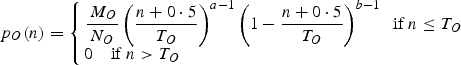 |
A.5 |
where TO is the duration in growth cycles over which the organ grows, and is an input parameter of the model. NO is a factor used to normalize the beta-function.
DPB(t) is the demand of potential buds. It is the sum of their sink strengths:
 |
A.6 |
(4) Biomass allocation
The amount of biomass computed with eqn (A.2) is allocated to the growing plant parts according to a proportional model (currently, we do not consider long-term storage or reserve remobilization in the model). The following rules are defined for each type of organ.
The root system receives pR(t)Q(t)/D(t).
The amount of biomass used for secondary growth is DC(t)Q(t)/D(t).
Each growing organ, O, of chronological age n receives pO(n)Q(t)/D(t).
All the potential buds receive QPB(t) = DPB(t)Q(t)/D(t). We note that QPB(t)/DPB(t) = Q(t)/D(t).
The equations of biomass allocation give the increase in biomass of the existing organs of the plant. They also reveal the importance of the ratio of biomass to demand in the allocation process, which leads us to consider this ratio as the key variable to control plant organogenesis. The following section describes the corresponding equations.
(5) Determination of the number of organs
From the amount of biomass allocated to the potential buds, we determine the number of active buds and then the number of the different kinds of organs in each growth unit.
The number of active buds, bkl(t), in a phytomer mkl(t, 1) is given by eqn (5):
| A.7 |
This allows us to compute the demand of the active buds, DFB(t):
 |
A.8 |
Equation (6) or (A.9) gives the amount of biomass allocated to each active bud of physiological age k in order to build the organs generated in the corresponding growth unit:
| A.9 |
This ratio controls several topological events:
(a) the branch life span, τk(t), for a branch of physiological age k born at cycle t (eqn 7 or A.10):
| A.10 |
(b) the number of phytomers ukl(t + 1) of type mkl(t + 1,1) (eqn 8 or A.11):
 |
A.11 |
(c) the number of fruits uF,k (t + 1) in a growth unit of physiological age k born at cycle t + 1 (eqn 9 or A.12)
 |
A.12 |
The number of organs appearing at cycle t + 1 is thus determined, which ends the growth cycle t. The following growth cycle starts with the appearance of the new organs. As their volumes and dimensions are known, the biomass production at cycle t + 1 can be deduced from the total leaf surface area, and so on.
LITERATURE CITED
- Balandier P, Lacointe A, Le Roux X, Sinoquet H, Cruiziat P, Le Dizès S. SIMWAL: a structural–functional model simulating single walnut tree growth in response to climate and pruning. Annals of Forest Science. 2000;57:571–585. [Google Scholar]
- Barthélémy D, Caraglio Y. Plant architecture: a dynamic, multilevel and comprehensive approach of plant form, structure and ontogeny. Annals of Botany. 2007;99:375–407. doi: 10.1093/aob/mcl260. [DOI] [PMC free article] [PubMed] [Google Scholar]
- Barthélémy D, Caraglio Y, Costes E. Architecture, gradients morphogénétiques et âge physiologique chez les végétaux. In: Bouchon J, de Reffye P, Barthélémy D, editors. Modélisation et simulation de l'architecture des végétaux. Montpellier, France: INRA; 1997. pp. 89–136. Science Update. [Google Scholar]
- Bell A. Plant form. An illustrated guide to flowering plant morphology. Oxford: Oxford University Press; 1991. [Google Scholar]
- Blaise F, de Reffye P. Simulation de la croissance des arbres et influence du milieu: le logiciel AMAPPara. In: Tankoano J., editor. Colloque africain sur la recherche en informatique. Vol. 2. Paris: ORSTOM; 1994. pp. 61–75. (CARI94) [Google Scholar]
- Borchert R, Honda H. Control of development in the bifurcating branch system of tabebuia rosea. Botanical Gazette. 1984;142:394–401. [Google Scholar]
- Buck-Sorlin G, Kniemeyer O, Kurth W. Barley morphology, genetics and hormonal regulation of internode elongation modelled by a relational growth grammar. New Phytologist. 2005;166:859–867. doi: 10.1111/j.1469-8137.2005.01324.x. [DOI] [PubMed] [Google Scholar]
- Buck-Sorlin G, Hemmerling R, Kniemeyer O, Burema B, Kurth W. A rule-based model of barley morphogenesis with special respect to shading and gibberellic acid signal transduction. Annals of Botany. 2008;101:1109–1123. doi: 10.1093/aob/mcm172. [DOI] [PMC free article] [PubMed] [Google Scholar]
- Cournède PH, Kang M, Mathieu A, et al. Structural factorization of plants to compute their functional and architectural growth. Simulation. 2006;82:427–438. [Google Scholar]
- Cournède PH, Mathieu A, Houllier F, Barthélémy D, de Reffye P. Computing competition for light in the GreenLab model of plant growth: a contribution to the study of the effects of density on resource acquisition and architectural development. Annals of Botany. 2008;101:1207–1219. doi: 10.1093/aob/mcm272. [DOI] [PMC free article] [PubMed] [Google Scholar]
- Deleuze C. Pour une dendrométrie fonctionnelle: essai sur l'intégration de connaissances écophysiologiques dans les modèles de production ligneuse. Lyon I, France: University Claude Bernard; 1996. PhD Thesis. [Google Scholar]
- Drouet J, Pagès L. GRAAL: a model of GRowth Architecture and carbon ALocation during the vegetative phase of the whole maize plant, model description and parameterisation. Ecological Modelling. 2003;165:147–173. [Google Scholar]
- Eschenbach C. Emergent properties modelled with the functional structural tree growth model ALMIS: computer experiments on resource gain and use. Ecological Modelling. 2005;186:470–488. [Google Scholar]
- Evers J, Vos J, Fournier C, Andrieu B, Chelle M, Struik P. Towards a generic architectural model of tillering in graminae, as exemplified by spring wheat (Tricitum aestivum) New Phytologist. 2005;166:801–812. doi: 10.1111/j.1469-8137.2005.01337.x. [DOI] [PubMed] [Google Scholar]
- Fourcaud T, Zhang X, Stokes A, Lambers H, Körner C. Plant growth modelling and applications: the increasing importance of plant architecture in growth models. Annals of Botany. 2008;101:1053–1063. doi: 10.1093/aob/mcn050. [DOI] [PMC free article] [PubMed] [Google Scholar]
- Gautier H, Mech R, Prusinkiewicz P, Varlet-Grancher C. 3D architectural modelling of aerial photomorphogenesis in white clover (Trifolium Repens L.) using L-systems. Annals of Botany. 2000;85:359–370. [Google Scholar]
- Godin C, Sinoquet H. Functional–structural plant modelling. New Phytologist. 2005;166:705–708. doi: 10.1111/j.1469-8137.2005.01445.x. [DOI] [PubMed] [Google Scholar]
- Godin C, Guédon Y, Costes E. Exploration of a plant architecture database with the AMAPmod software illustrated on an apple tree hybrid family. Agronomie. 1999;19:163–184. [Google Scholar]
- Grosfeld J, Barthélémy D, Brion C. Architectural variations of Araucaria araucana (Molina) K. Koch (Araucariaceae) in its natural habitat. In: Kurmann MH, Hemsley AR, editors. The evolution of plant architecture. Kew, London: Kew Publishing; 1999. pp. 109–122. [Google Scholar]
- Guédon Y, Barthélémy D, Caraglio Y, Costes E. Pattern analysis in branching and axillary flowering sequences. Journal of Theoretical Biology. 2001;212:481–520. doi: 10.1006/jtbi.2001.2392. [DOI] [PubMed] [Google Scholar]
- Guo Y, Ma Y, Zhan Z, et al. Parameter optimization and field validation for the functional–structural model GreenLab for maize. Annals of Botany. 2006;97:217–230. doi: 10.1093/aob/mcj033. [DOI] [PMC free article] [PubMed] [Google Scholar]
- Hallé F, Martin R. Etude de la croissance rythmique chez l'hévéa (Hevea brasiliensis Mull. Arg.) Adansonia. 1968;8:475–503. [Google Scholar]
- Hallé F, Oldeman R, Tomlinson P. Tropical trees and forests, an architectural analysis. New York: Springer-Verlag; 1978. [Google Scholar]
- Heuret P, Barthélémy D, Nicolini E, Atger C. Analyse des composantes de la croissance en hauteur et de la formation du tronc chez le chêne sessile, Quercu petraea (Matt.) Liebl. (Fagaceae) en sylvicutlture dynamique. Canadian Journal of Botany. 2000;78:361–373. [Google Scholar]
- Heuret P, Meredieu C, Coudurier T, Courdier F, Barthélémy D. Ontogenetic trends in the morphological features of main stem annual shoots of Pinus pinaster (Pinaceae) American Journal of Botany. 2006;93:1577–1587. doi: 10.3732/ajb.93.11.1577. [DOI] [PubMed] [Google Scholar]
- Heuvelink E. Dry matter partitioning in a tomato plant: one common assimilate pool? Journal of Experimental Botany. 1995;46:1025–1033. [Google Scholar]
- Kang M, Cournède PH, de Reffye P, Auclair D, Hu BG. Analytical study of a stochastic plant growth model: application to the GreenLab model. Mathematics and Computers in Simulation. 2008;78:57–75. [Google Scholar]
- de Kroon H, Huber H, Stuefer J, van Groenedael J. A modular concept of phenotypic plasticity in plants. New Phytologist. 2005;166:73–82. doi: 10.1111/j.1469-8137.2004.01310.x. [DOI] [PubMed] [Google Scholar]
- Kurth W, Sloboda B. Growth grammars simulating trees – an extension of Lsystems incorporating local variables and sensitivity. Silva Fennica. 1997;31:285–295. [Google Scholar]
- Lacointe A. Carbon allocation among tree organs: a review of basic processes and representation in functional–structural models. Annals of Forest Science. 2000;57:521–533. [Google Scholar]
- Lacointe A, Isebrands JG, Host GE. A new way to account for the effect of source–sink spatial relationships in whole plant carbon allocation models. Canadian Journal of Forest Research. 2002;32:1838–1848. [Google Scholar]
- Lanner R. On the intensivity of height growth to spacing. Forest Ecology and Management. 1985;13:143–148. [Google Scholar]
- Le Roux X, Lacointe A, Escobar-Gutiérrez A, Le Dizès S. Carbon-based models of individual tree growth: a critical appraisal. Annals of Forest Science. 2001;58:469–506. [Google Scholar]
- Letort V, Cournède PH, Mathieu A, de Reffye P, Constant T. Parametric identification of a functional–structural tree growth model and application to beech trees (Fagus sylvatica, Fagaceae) Functional Plant Biology. 2008;35:951–963. doi: 10.1071/FP08065. [DOI] [PubMed] [Google Scholar]
- Lusk C, Le-Quesne C. Branch whorls of juveniles Araucaria araucana (Molina) Koch: are they formed annually? Revista Chilena de Historia Natural. 2000;73:497–502. [Google Scholar]
- Marcelis L. The dynamics of growth and dry matter distribution in cucumber. Annals of Botany. 1992;69:487–492. [Google Scholar]
- Marcelis L. A simulation model for dry matter partitioning in cucumber. Annals of Botany. 1994;74:43–52. doi: 10.1093/aob/74.1.43. [DOI] [PubMed] [Google Scholar]
- Marcelis L. Sink strength as a determinant of dry matter partitioning in the whole plant. Journal of Experimental Botany. 1996;47:1281–1291. doi: 10.1093/jxb/47.Special_Issue.1281. [DOI] [PubMed] [Google Scholar]
- Marcelis L, Heuvelink E, Baan Hofman-Eijer L, Den Bakker J, Xue L. Flower and fruit abortion in sweet pepper in relation to source and sink strength. Journal of Experimental Botany. 2004;55:2261–2268. doi: 10.1093/jxb/erh245. [DOI] [PubMed] [Google Scholar]
- Mathieu A. Essai sur la modélisation des interactions entre la croissance et le développement d'une plante – cas du modèle GreenLab. France: Ecole Centrale de Paris; 2006. PhD Thesis. [Google Scholar]
- Mathieu A, Cournède PH, de Reffye P. A dynamical model of plant growth will full retroaction between organogenesis and photosynthesis. ARIMA. 2006;4:101–107. [Google Scholar]
- Mathieu A, Zhang B, Heuvelink E, Liu S, Cournède PH, de Reffye P. Calibration of fruit cyclic patterns in cucumber plants as a function of source–sink ratio with the Greenlab model. In: Prusinkiewicz P, Hanan J, Lane B., editors. Proceedings of the 5th International Workshop on Functional–Structural Plant Models; Napier, New Zealand. Hawke's Bay, New Zealand: 2007. pp. 31–34. Print Solutions. [Google Scholar]
- Mathieu A, Cournède PH, Barthélémy D, de Reffye P. Rhythms and alternating patterns in plants as emergent properties of a model of interaction between development and functioning. Annals of Botany. 2008;101:1233–1242. doi: 10.1093/aob/mcm171. [DOI] [PMC free article] [PubMed] [Google Scholar]
- Mech R, Prusinkiewicz P. Visual models of plant interacting with their environment. Computer Graphics (SIGGRAPH ‘96 Proceedings) 1996;30:397–410. [Google Scholar]
- Minchin P, Lacointe A. New understanding on phloem physiology and possible consequences for modelling long-distance carbon transport. New Phytologist. 2005;166:771–779. doi: 10.1111/j.1469-8137.2005.01323.x. [DOI] [PubMed] [Google Scholar]
- Nicolini E. Nouvelles observations sur la morphologie des unités de croissance du hêtre (Fagus Sylvatica L.). Symétrie des pousses, reflet de la vigueur des arbres. Canadian Journal of Botany. 2000;78:77–87. [Google Scholar]
- Nicolini E, Chanson B. La pousse courte, un indicateur du degré de maturation chez le hêtre (Fagus Sylvatica L.) Canadian Journal of Botany. 1999;77:1539–1550. [Google Scholar]
- Niklas K. The BIO-Logic and machinery of plant morphogenesis. American Journal of Botany. 2003;90:515–525. doi: 10.3732/ajb.90.4.515. [DOI] [PubMed] [Google Scholar]
- Novoplansky A. Hierarchy establishment among potentially similar buds. Plant, Cell and Environment. 1996;19:781–786. [Google Scholar]
- Perttunen J, Sievänen R, Nikinmaa E, Salminen H, Saarenmaa H, Väkevä J. Lignum: a tree model based on simple structural units. Annals of Botany. 1996;77:87–98. [Google Scholar]
- Perttunen J, Sievänen R, Nikinmaa E. Lignum: a model combining the structure and the functioning of trees. Ecological Modelling. 1998;108:189–198. [Google Scholar]
- Prusinkiewicz P, Hammel M, Hanan J, Mech R. L-system: from the theory to visual models of plants. In: Michalewicz MT, editor. Proceedings of the 2nd CSIRO Symposium on Computational Challanges in Life Sciences. Melbourne: CSIRO Publishing; 1997. pp. 1–27. [Google Scholar]
- Prusinkiewicz P, Smith R, Leyser O. Apical dominance models can generate basipetal patterns of bud activation. In: Prusinkiewicz P, Hanan J, Lane B., editors. Proceedings of the 5th International Workshop on Functional–Structural Plant Models; Napier, New Zealand. Hawke's Bay, New Zealand: 2007. pp. 48–52. Print Solutions. [Google Scholar]
- de Reffye P. Modélisation de l'architecture des arbres par des processus stochastiques. Simulation spatiale des modèles tropicaux sous l'effet de la pesanteur. Application au coffea robusta. France: Université Paris-Sud, Centre d'Orsay; 1979. Ph.D. thesis. [Google Scholar]
- de Reffye P, Hu B. Relevant choices in botany and mathematics for building efficient dynamic plant growth models: GreenLab case. In: Hu BG, Jaeger M, editors. International Symposium on Plant Growth Modeling, Simulation, Visualization and their Applications – PMA’03. Beijing, China: Tsinghua University Press and Springer; 2003. pp. 87–107. [Google Scholar]
- de Reffye P, Fourcaud T, Blaise F, Barthélémy D, Houllier F. A functional model of tree growth and tree architecture. Silva Fennica. 1997;31:297–311. [Google Scholar]
- de Reffye P, Goursat M, Quadrat J, Hu B. The dynamic equations of the tree morphogenesis GreenLab model. Rocquencourt, France: INRIA; 2003. Technical Report 4877. [Google Scholar]
- de Reffye P, Heuvelink E, Barthélémy D, Cournède PH. Plant growth models. In: Jorgensen SE, Fath BD, editors. Encyclopedia of ecology. vol. 4. Amsterdam: Elsevier; 2008. pp. 2824–2838. P–S. [Google Scholar]
- Remphrey W, Davidson C. Shoot preformation in clones of Fraxinus pennsylvanica in relation to site and year of bud formation. Trees. 1994;8:126–131. [Google Scholar]
- Rickman R, Klepper B. The phyllochron: where do we go in the future? Crop Science. 1995;35:44–49. [Google Scholar]
- Rolland-Lagan A, Federl P, Prusinkiewicz P. Reviewing models of auxin canalisation in the context of vein pattern formation in Arabidopsis leaves. In: Godin C, et al., editors. Proceedings of the 4th International Workshop on Functional-Structural Plant Models, Montpellier. 2004. pp. 376–381. [Google Scholar]
- Sabatier S, Barthélémy D. Bud structure in relation to shoot morphology and position on the vegetative annual shoots of Juglans regia L. (Juglandaceae) Annals of Botany. 2001;87:117–123. [Google Scholar]
- Shinozaki K, Yoda K, Hozumi K, Kira T. A quantitative analysis of plant form – the pipe model theory. i. Basic analysis. Japanese Journal of Ecology. 1964;14:97–105. [Google Scholar]
- Siarry P, Dreyfus G. La méthode du recuit simulé. Paris: IDSET; 1988. [Google Scholar]
- Sievänen R, Nikinmaa E, Nygren P, Ozier-Lafontaine H, Perttunen J, Hakula H. Components of a functional–structural tree model. Annals of Forest Sciences. 2000;57:399–412. [Google Scholar]
- Sims D, Luo Y, Seemann J. Importance of leaf versus whole-plant CO2 environment for photosynthetic acclimation. Plant, Cell and Environment. 1998;21:1189–1196. [Google Scholar]
- Stafstrom J. Developmental potential of shoots buds. In: Gartner BL, editor. Plant stems: physiology and functional morphology. San Diego: Academic Press; 1995. pp. 257–279. [Google Scholar]
- Sultan S. Phenotypic plasticity for plant development, function and life history. Trends in Plant Science. 2000;5:537–542. doi: 10.1016/s1360-1385(00)01797-0. [DOI] [PubMed] [Google Scholar]
- Sultan S. Promising research directions in plant phenotypic plasticity. Perspectives in Plant Ecology, Evolution, and Systematics. 2004;6:227–233. [Google Scholar]
- Varlet-Grancher C, Gosse G, Chartier M, Sinoquet H, Bonhomme R, Allirand JM. Mise au point: rayonnement solaire absorbé ou intercepté par un couvert végétal. Agronomie. 1989;9:419–439. [Google Scholar]
- Vose J, Sullivan N, Clinton B, Bolstad P. Vertical leaf area distribution, light transmittance, and application of the Beer–Lambert law in four mature hardwood stands in the southern Appalachians. Canadian Journal of Forest Research. 1995;25:1036–1043. [Google Scholar]
- Walter E, Pronzato L. Identification de modèles paramétriques. Paris: Masson; 1994. [Google Scholar]
- Wardlaw I. The control of carbon partitioning in plants. New Phytologist. 1990;16:341–381. doi: 10.1111/j.1469-8137.1990.tb00524.x. [DOI] [PubMed] [Google Scholar]
- Warren-Wilson J. Control of crop processes. In: Rees AR, Cockshull KE, Hand DW, Hurd RG, editors. Crop processes in controlled environments. London: Academic Press; 1972. pp. 7–30. [Google Scholar]
- White J. The plant as a metapopulation. Annual Review of Ecology and Systematics. 1979;10:109–145. [Google Scholar]
- Yan H, Kang M, De Reffye P, Dingkuhn M. A dynamic, architectural plant model simulating resource-dependent growth. Annals of Botany. 2004;93:591–602. doi: 10.1093/aob/mch078. [DOI] [PMC free article] [PubMed] [Google Scholar]
- Yin XY, Goudriaan J, Lantinga EA, Vos J, Spiertz HJ. A flexible sigmoid function of determinate growth. Annals of Botany. 2003;91:361–371. doi: 10.1093/aob/mcg029. [DOI] [PMC free article] [PubMed] [Google Scholar]