A graphical algorithm for fast computation of identity coefficients and generalized kinship coefficients

Abstract

Summary: Computing the probability of identity by descent sharing among n genes given only the pedigree of those genes is a computationally challenging problem, if n or the pedigree size is large. Here, I present a novel graphical algorithm for efficiently computing all generalized kinship coefficients for n genes. The graphical description transforms the problem from doing many recursion on the pedigree to doing a single traversal of a structure referred to as the kinship graph.

Availability: The algorithm is implemented for n = 4 in the software package IdCoefs at http://home.uchicago.edu/abney/Software.html.

Contact: abney@bsd.uchicago.edu

Supplementary Information:Supplementary data are available at Bioinformatics online.

1 INTRODUCTION

The expected amount of genetic identity among a group of individuals is determined by their genetic relationship and is essential in describing the probabilistic interdependence of both genotypes and phenotypes within the group. For instance, given a multivariate normal trait, the dependence between any two individuals is fully determined by the covariance matrix, which, in turn, depends on their degree of relatedness. For non-normal traits, higher order moments involving larger sets of individuals will, generally, be needed. For a pair of individuals, the genetic relatedness is well described by the detailed identity coefficients (Gillois, 1964; Harris, 1964), that specify, given the four genes of the two individuals at a single locus, the probabilities of each way of partitioning the four genes into groups of identical by descent (IBD) genes. The number of detailed identity coefficients for n genes, however, is given by the n-th Bell number and increases rapidly with the number of individuals being considered. For three individuals, for instance, there are 203 detailed identity coefficients, while for four individuals there are 4140 (Thompson, 1974) (or 66 and 712 if we ignore whether a gene is maternally or paternally inherited).

To compute the condensed identity coefficients (i.e. ignoring maternal and paternal inheritance information), one takes a linear combination of generalized kinship coefficients, a generalization of the kinship coefficient to more than two genes. While the standard kinship coefficient is the probability that two randomly drawn genes are IBD, when there are multiple genes there are multiple generalized kinship coefficients where each kinship coefficient is the probability for a particular subset of genes being IBD (Lange and Sinsheimer, 1992; Weeks and Lange 1988). Note that the generalized kinship coefficients differ from identity coefficients only in that in the former, genes are drawn with replacement from an individual, while in the latter the genes are drawn without replacement. Typically, identity coefficients are used to describe the probabilities of a pair of individuals (or possibly more) having their genes in a particular IBD configuration, whereas generalized kinship coefficients are the probabilities of some set of randomly drawn genes being IBD. The generalized kinship coefficients are determined from straightforward recursive (Harris, 1964; Karigl, 1981; Lange and Sinsheimer, 1992; Weeks and Lange, 1988) or path counting (Cheng et al., 2008; Wright, 1922) algorithms. Executing many recursions, however, one for each generalized kinship coefficient, can be time consuming when the pedigree is large or if identity coefficients for more than two individuals are desired. Here, I present a novel, graphical approach to the problem of computing generalized kinship coefficients that replaces the need for multiple recursions with a single traversal through a graph whose structure is determined by the pedigree.

2 METHODS

To compute the generalized kinship coefficients, first consider n genes drawn with replacement from n not necessarily distinct individuals. We define a graph called an identity graph (IG) by considering these n genes as nodes with an edge between nodes representing IBD. That is, genes that are connected in the IG are necessarily IBD. The set of all possible IGs constitutes the sample space of a random variable X which takes on value i when the IBD pattern among the genes is described by the i-th IG. Note that the probability mass function (PMF) of X, p(X), gives the N_IG generalized kinship coefficients for the n genes, where N_IG is the number of IGs.

We now define the notion of a kinship graph (KG). To each node v in the we associate n genes and a random variable X_v. Each gene in v is considered a random draw with replacement from the two genes of an individual in the pedigree. Note that the possible partitions of the n genes into connected components is represented by a particular IG with the probability of each partition given by the PMF p(X_v) (see the Supplementary Materials for additional details). Because each gene in node v is itself a copy of a gene from one of the parents of the individual, there is a relationship between v and another node u in which the genes from a single individual in v are replaced by genes from that individual's parents in u. This relationship defines an edge between v and u, and is discussed in greater detail below. In the notation that follows, each individual in the pedigree is numbered such that a parent's number is always less than a child's number, and each gene is given a gene identifier (GID) equal to the number of the individual from whom it was drawn. That is, the GID represents an individual. For instance, in the case of n = 4 let node v have genes (5, 5, 3, 3), meaning that the first two genes (each with a GID of 5) are drawn randomly (with replacement) from individual 5 and the last two genes are drawn from individual 3. Genes from an individual represented multiple times in a node may represent multiple distinct draws from that individual or jointly represent a single draw (i.e. a single gene is drawn and each GID refers to that gene). GIDs representing a single draw are given identical subscripts and are called connected (i.e. they form a connected component). So, for instance the node (5₁, 5₁, 5₂, 5₂) has the first two genes connected and the second two genes connected, although these two connected components may or may not be IBD with each other (i.e. they represent two draws with replacement from individual 5). Using the above principle, given an initial node v, we can construct a KG in the following way.

1. Select the largest GID g from the genes in the node. Let k be the number of connected components with that GID and f(g) and m(g) be the father and mother of g. Node v then has 2^k child nodes c_i(v), i = 1,…, 2^k, where in each child node every occurrence of g is replaced with either f(g) or m(g) with the requirement that every gene in a connected component be replaced with the same parental GID.

2. A node also consists of a set of constraints on the PMF of X that can be thought of in the following way. When identifying v' child nodes, if multiple occurrences of a GID at node v get replaced by the same parental GID, those genes in the child node are connected and necessarily IBD (e.g. the maternal gene from the repeated individual is chosen multiple times). This restricts the PMF of X_c(v) to be zero for values corresponding to IGs for which those genes are not connected. Examples are given in the Supplementary Materials.

3. The PMF of X_v is a weighted sum of the PMFs of v's child nodes, 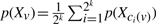, where 2^k is the number of child nodes of v and c_i(v) is v's i-th child node.

Repeating these steps allows one to recursively construct the KG given some initial node. Note that child nodes of different parent nodes are not necessarily distinct. For instance, if individual 6 is a sibling to individual 5 then the child nodes of (6, 6, 3, 3) are identical to the child nodes of (5, 5, 3, 3).

A terminal node of the KG is one where all GIDs of the node represent founders of the pedigree. At a terminal node t the PMF of X_t must be determined from the following boundary conditions:

• Boundary Condition 1: If at a terminal node t, all genes with the same GID are connected (i.e. they are all in a single connected component), then, letting S(t) be the IG such that genes with connected GIDs are IBD and genes with disconnected GIDs are not IBD, .

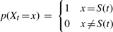• Boundary Condition 2: If a terminal node t has genes from a single founder that are not connected (i.e. they are not all in a single connected component), then, letting R be the IG defined by the connectedness of the GIDs at t, 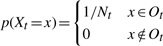, where O_t={identity graphs S ∣ genes in S from distinct founders are disconnected and S is compatible with R} and N_t=|O_t|.

In the second condition, we define an IG B as being compatible with A if all genes that are connected in A are also connected in B. These boundary conditions establish the PMF of X at the terminal nodes of the KG, which, in turn, are used to compute the PMFs at the parents of the terminal nodes using Step 3 above. This process is repeated iteratively until the distribution at the desired node is known. Further explanations of the KG and the equivalence of the algorithm proposed here to the recursive algorithms of Weeks and Lange 1988, as well as examples of the boundary conditions and the construction of a KG are given in the Supplementary Materials.

3 DISCUSSION

The graphical algorithm for computing generalized kinship coefficients described here allows for computational advantages over the more traditional recursive methods (Harris, 1964; Karigl, 1981; Lange and Sinsheimer, 1992; Weeks and Lange, 1988). For instance, it is possible to compute all the generalized kinship coefficients essentially simultaneously. That is, in the traditional approach a recursion must be done for each desired kinship coefficient. As n increases, the number of kinship coefficients can quickly grow to enormous sizes (Thompson, 1974), resulting in highly burdensome computations. With the algorithm proposed here, the recursion to construct the KG is done only once, at which time all kinship coefficients are computed. Nevertheless, finding an efficient algorithm for traversing the KG is itself a non-trivial problem. In particular, when either the pedigree or the number of genes becomes large, the size of the KG can become bigger than what may easily be stored in computer memory. The current software implementation considers the four-genes case and uses a depth-first search strategy to recursively traverse the graph. A hash table is used to store information from visited nodes with nodes that have not been recently referenced discarded in favor of newly visited nodes, if a specified amount of memory is exceeded. It is likely, however, that more efficient dynamic programming algorithms could be used.

The algorithm is implemented in the software package IdCoefs, is written in ISO C, and should compile on any platform that has a compliant compiler. The software has been tested on both 32-bit and 64-bit Mac and Linux platforms. The package computes the condensed identity coefficients for pairs of individuals by finding all generalized kinship coefficients for four autosomal genes. Extensions to more genes or sex-linked genes is straightforward but not currently implemented. We tested the current version of IdCoefs, which uses the algorithm described here, against an older version based on the recursion relations of Karigl, 1981. The test used a 13 generation pedigree comprising 3028 individuals and computed the identity coefficients for all pairs of 10 individuals (55 pairs). The current version of IdCoefs took 2 min 13 s on a Macintosh with a 2 GHz G5 processor, while the old version took 29 min 49 s, both versions were allowed to use 1 GB of RAM. The current software has been used to compute the identity coefficients for all pairs of 3555 individuals in a single 13 generation Hutterite pedigree (6 320 790 pairs) which have been used to estimate covariances and, hence, heritabilities of quantitative traits (e.g. Weiss et al., 2006) and to test Hardy–Weinberg equilibrium (Bourgain et al., 2004). Additionally, the software has been used in other populations with large pedigrees (Angius et al., 2008; McArdle et al., 2007), and has been adapted into an R package by Na Li (http://cran.r-project.org/web/packages/identity/index.html).

Funding: National Institutes of Health (HG02899).

Conflict ot Interest: none declared.

REFERENCES

- Angius A, et al. Patterns of linkage disequilibrium between SNPs in a sardinian population isolate and the selection of markers for association studies. Hum. Hered. 2008;65:9–22. doi: 10.1159/000106058. [DOI] [PubMed] [Google Scholar]
- Bourgain C, et al. Testing for Hardy-Weinberg equilibrium in samples with related individuals. Genetics. 2004;168:2349–2361. doi: 10.1534/genetics.104.031617. [DOI] [PMC free article] [PubMed] [Google Scholar]
- Cheng E, et al. Scalable computation of kinship and identity coefficients on large pedigrees. In: Markstein P, Xu Y, editors. Proceedings of the Computational Systems Bioinformatics 2008 Conference. Vol. 7. London: Imperial College Press; 2008. pp. 27–36. [PubMed] [Google Scholar]
- Gillois M. La relation d'identité en génétique. Ann. Inst. Henri Poincaré B. 1964;2:1–94. [Google Scholar]
- Harris DL. Genotypic covariances between inbred relatives. Genetics. 1964;50:1319–1348. doi: 10.1093/genetics/50.6.1319. [DOI] [PMC free article] [PubMed] [Google Scholar]
- Karigl G. A recursive algorithm for the calculation of identity coefficients. Ann. Hum. Genet. 1981;45:299–305. doi: 10.1111/j.1469-1809.1981.tb00341.x. [DOI] [PubMed] [Google Scholar]
- Lange K, Sinsheimer JS. Calculation of genetic identity coefficients. Ann. Hum. Genet. 1992;4:339–346. doi: 10.1111/j.1469-1809.1992.tb01162.x. [DOI] [PubMed] [Google Scholar]
- McArdle PF, et al. Homozygosity by descent mapping of blood pressure in the old order amish: evidence for sex specific genetic architecture. BMC Genet. 2007;8:66. doi: 10.1186/1471-2156-8-66. [DOI] [PMC free article] [PubMed] [Google Scholar]
- Thompson EA. Gene identities and multiple relationships. Biometrics. 1974;30:667–680. [PubMed] [Google Scholar]
- Weeks DE, Lange K. The affected-pedigree-member method of linkage analysis. Am. J. Hum. Genet. 1988;42:315–326. [PMC free article] [PubMed] [Google Scholar]
- Weiss LA, et al. The sex-specific genetic architecture of quantitative traits in humans. Nat. Genet. 2006;38:218–222. doi: 10.1038/ng1726. [DOI] [PubMed] [Google Scholar]
- Wright S. Coefficients of inbreeding and relationship. Am. Nat. 1922;56:330–338. [Google Scholar]