Assessing phylogenetic motif models for predicting transcription factor binding sites

Abstract

Motivation: A variety of algorithms have been developed to predict transcription factor binding sites (TFBSs) within the genome by exploiting the evolutionary information implicit in multiple alignments of the genomes of related species. One such approach uses an extension of the standard position-specific motif model that incorporates phylogenetic information via a phylogenetic tree and a model of evolution. However, these phylogenetic motif models (PMMs) have never been rigorously benchmarked in order to determine whether they lead to better prediction of TFBSs than obtained using simple position weight matrix scanning.

Results: We evaluate three PMM-based prediction algorithms, each of which uses a different treatment of gapped alignments, and we compare their prediction accuracy with that of a non-phylogenetic motif scanning approach. Surprisingly, all of these algorithms appear to be inferior to simple motif scanning, when accuracy is measured using a gold standard of validated yeast TFBSs. However, the PMM scanners perform much better than simple motif scanning when we abandon the gold standard and consider the number of statistically significant sites predicted, using column-shuffled ‘random’ motifs to measure significance. These results suggest that the common practice of measuring the accuracy of binding site predictors using collections of known sites may be dangerously misleading since such collections may be missing ‘weak’ sites, which are exactly the type of sites needed to discriminate among predictors. We then extend our previous theoretical model of the statistical power of PMM-based prediction algorithms to allow for loss of binding sites during evolution, and show that it gives a more accurate upper bound on scanner accuracy. Finally, utilizing our theoretical model, we introduce a new method for predicting the number of real binding sites in a genome. The results suggest that the number of true sites for a yeast TF is in general several times greater than the number of known sites listed in the Saccharomyces cerevisiae Database (SCPD). Among the three scanning algorithms that we test, the MONKEY algorithm has the highest accuracy for predicting yeast TFBSs.

Contact: j.hawkins@imb.uq.edu.au

1 INTRODUCTION

An important goal in current molecular biology research is to understand the cellular systems that regulate gene expression. One part of this goal lies in identifying the binding locations of transcription factors (TFs)—proteins that bind to DNA segments and regulate the expression of nearby genes. Due to the difficulty in accurately assaying protein–DNA interactions on a large scale, we have only a small amount of high-quality experimental data regarding the location of these binding sites. Hence, we require good computational tools for identifying the remaining sites.

Unfortunately, attempts to construct accurate binding site predictors have been frustrated by the small size of the binding sites, which means that DNA regions identical to functional binding sites occur by chance with high frequency. As a result, standard probabilistic motif search using a position weight matrix (PWM) suffers from overwhelming numbers of false positive predictions (Wasserman and Sandelin, 2004). In order to produce better predictors, researchers have turned to other sources of information.

The biological reality is that many components of the cellular system cooperate to produce a protein–DNA binding event. For example, TFs tend to bind in groups to form macro-molecular complexes, and the binding is thus stabilized by the presence of other TFs (Levine and Tjian, 2003). Furthermore, there is emerging evidence that a range of epigenetic factors contribute to the binding of TFs (Guccione et al., 2006; Kouzarides, 2007; Liu et al., 2006). Computational tools have been constructed that make use of TF protein complex information (Berman et al., 2002) and epigenetic DNA modifications (Narlikar et al., 2007; Whitington et al., 2008).

An alternative source of information, which is not exploited by the cell itself, comes from comparative genomics. We expect that important features in biological sequences tend to evolve more slowly than the neutral rate. This assumption has been exploited to identify functional regions by comparative genomics techniques such as phylogenetic footprinting (Gumucio et al., 1992) and shadowing (Boffelli et al., 2003). The assumption of evolutionary conservation has also been utilized by a class of motif scanning algorithms based on what we call phylogenetic motif models (PMMs). These models extend the popular PWM motif models used in computational biology to represent and identify sequence features such as TF binding sites (TFBSs), splice junctions and binding domains in DNA, RNA and protein molecules, respectively (GuhaThakurta, 2006; Stormo, 2000). Whereas a PWM computes the probability of given region in a single genome being an instance of a motif, a PMM computes the probability of an ungapped region in a multiple alignment being comprised of instances of the motif that evolved independently from an ancestral instance.

PMM scanning algorithms are an extension of simple PWM scanning algorithms. Instead of scanning a single sequence, however, a PMM algorithm scans a multiple alignment of orthologous sequences, usually produced by a tool such as ClustalW (Chenna et al., 2003), MAFFT (Katoh et al., 2002), MULTIZ (Blanchette et al., 2004) or Multi-LAGAN (Brudno et al., 2003). The PMM scanning approach also requires an explicit model of nucleic acid substitution and a phylogenetic tree describing the relationship and evolutionary distances among the species from which the orthologous sequences are taken. Several TFBS prediction algorithms have been implemented that use PMMs. These include the Monkey algorithm (Moses et al., 2004), a variant called rMonkey (Moses et al., 2006), and Motiph, which is available as part of the MEME Suite (http://meme.nbcr.net).

Surprisingly, earlier attempts to demonstrate that these PMM scanning algorithms are superior to simple PWM scanners failed to show any significant difference (Hawkins and Bailey, 2008). In that work, we evaluated the algorithms using TF motifs, multiple alignments and known TFBSs from yeast (Saccharomyces cerevisiae). In addition to indicating that simple PWM scanning might be as accurate (at least in yeast) as PMM scanning, the accuracy of PMM scanners at predicting the known binding sites was orders of magnitude less than it should theoretically be, assuming that binding sites are not lost and that the multiple alignments are reasonably accurate.

One explanation for why the accuracy of PMM scanners appeared no better than that of simple PWM scans in previous work is that the gold standard might be biased against more sensitive scanning methods. One way in which this could happen is if the experimental methods used in creating the sets of known TFBSs systematically leave out weakly binding sites. Such weak sites will tend to have low PWM scores, and be missed by PWM scanners. However, weak sites are known to be important biologically (Gertz et al., 2008), so they will tend to be conserved, causing PMM scanners to detect them. If weak sites are systematically more likely to be missing from the gold standard, PMM scanners will appear to be less accurate (due to larger numbers of apparent false positive predictions—the weak-but-real sites) than simple PWM scanners.

Missing functional sites in the gold standard would also explain some, but not all, of the discrepancy between the theoretical and empirical accuracy of PMM scanners. Our earlier simplifying assumption that binding sites have not been lost in some of the orthologous species in the multiple alignment is clearly false (Moses et al., 2006). Relaxing this assumption in the theoretical model would lower the theoretically achievable prediction accuracy because loss-of-site events make real sites harder to distinguish from background sequence. Errors in the multiple alignments of orthologous species would also account for some of the discrepancy in accuracy, and the assumption that the multiple alignments correctly align orthologous positions is clearly overly optimistic.

The contributions of the present work are 4-fold. First, we extend our previous study of the empirical accuracy of PMM-based scanners using a set of known sites (a ‘gold standard’), confirming the apparent paradox noted above. Secondly, we show that the paradox disappears when we adopt an alternative evaluation approach that uses column-shuffled (‘random’) motifs, rather than a set of known sites, to measure prediction accuracy. Under this metric, PMM scanners are more accurate than a simple PWM scan, and heuristics for locally correcting errors in the multiple alignments are beneficial. Thirdly, we extend our theoretical model of PMM scanner accuracy to allow for site loss and and show that it more accurately fits the available data for yeast. Finally, we show how theoretical models of prediction accuracy can be used to estimate the number of functional binding sites of a TF in a genome, and provide such estimates for 21 yeast TFs.

2 MATERIALS AND METHODS

2.1 TFBS prediction algorithms

All the binding site prediction algorithms in this study use a matrix representation of a motif, M, in which the rows represent each of the four possible nucleic acids and the columns correspond to positions within the motif. Each matrix entry is the probability of seeing the given residue in the specified position. The algorithms all make use of a background distribution of nucleic acids, B, a single vector that contains the overall frequencies of the nucleic acids in the target genome. The PMM algorithms also require a phylogenetic tree with distances (in substitutions per site), relating the species in the alignments of orthologous regions that they scan.

Scoring a site using a PMM involves computing a log-likelihood ratio of an alignment column σ of N sequences given evolutionary models of the motif and background θ_M and θ_B, respectively. Under the assumption that the columns of the motif model are independent, the log-likelihood scores are additive; hence, the scoring function generalizes easily to the score for an alignment of length L by summing the scores of the individual columns. When aligned with the j-th position in the motif, the log-likelihood score for this column is written as

(1)

where θ_M^j refers to the motif model for the j-th position in the motif and T is a phylogenetic tree containing the evolutionary distances between the species. The two models θ_M and θ_B incorporate the frequencies in the position-specific probability matrix of the motif, M, the background frequencies of the residues, B, different substitution rates for the two models R_M and R_B, respectively, and an evolutionary model for calculating the substitution probabilities. We use the HKY (Hasegawa et al., 1985) model with the Halpern–Bruno modification (Halpern and Bruno, 1998) (HKY+HB) with all PMM scanning algorithms in this study.

The PMM scanning algorithms that we test differ primarily in how they handle gaps. The Motiph algorithm simply ignores regions with gaps. The MONKEY (Moses et al., 2004) and rMonkey (Moses et al., 2006) algorithms treat gaps as mistakes in the multiple alignment. MONKEY removes gaps locally, creating an ungapped local alignment for each position in the reference species. Each of these re-alignments can only use positions that are close to each other in the original multiple alignment. The rMonkey algorithm uses a slightly different heuristic for fixing gaps. Using the PWM model, it identifies the highest scoring site in the reference sequence, and then realigns it (without gaps) to the other sequences. Only regions that overlap the reference match by at least one base pair in the original multiple alignment are considered in the realignment. This process is repeated for the remaining binding-site free intervals in the reference sequence until no single species match remains that passes a significance threshold.

2.2 Measuring prediction accuracy

We measure the accuracy of TFBS prediction methods using false discovery rate (FDR), which expresses the proportion of the predictions that are false positives. We report accuracy as either FDR at a given sensitivity level or at a given number of predictions. In general, we are interested in knowing what the FDR is when we choose a particular score as a threshold for deciding which positions in the genome are predicted to be binding sites. Without loss of generality, assume that a prediction algorithm assigns a score, s, to a position in a genome, and that larger values of s indicate higher confidence that the position is a binding site.

When we evaluate prediction accuracy using a gold standard set of known sites, we define the FDR for each score threshold t such that there is at least one position with score t or larger as

(2)

where #S{s ≥ t} is the total number of positions in the genome whose score s, is at least t, and #N{s ≥ t} is the number of ‘negatives’ (non-binding positions) in the genome with score at least t.

When we evaluate prediction accuracy without reference to a set of known sites, we replace the numerator in Equation (2) with the expected number of negative predictions with score t or greater. This is simply np_t, where n is the total number positions scored, and p_t is the P-value of the score threshold. We estimate the P-value of score t using the empirical null score distribution we construct as described below in Section 2.4. This gives an (estimated) FDR of

(3)

We also make use of the q-value, a quantity closely related to FDR. The q-value is defined as the minimum FDR at which a score is deemed significant (Storey, 2002). Assuming, as before, that higher scores are more significant, the q-value of score t is therefore

(4)

2.3 Estimating prediction accuracy using known sites

The most straightforward way to compare binding site prediction algorithms is by estimating their ability to discriminate a known set of binding sites from non-binding sites. The Saccharomyces cerevisiae Database (SCPD) (Zhu and Zhang, 1999) contains sets of known binding sites in the S.cerevisiae genome for a number of TFs. We use only the 21 TFs whose sets contain at least five known sites. We build motifs for each of these TFs to measure the accuracy (FDR) of the scanning algorithms in a cross-validation setup. Using the set of sites for a single TF, we build a set of motifs in which, for each motif, exactly one of the sites is removed. Using each motif independently, we scan multiple alignments of all intergenic regions of four species of yeast, ignoring predictions for the sites we used in building that motif. We then compute the FDR at a given sensitivity level (percentage of positives predicted) of the combined predictions made using all of the motifs for the given TF, assuming that all positions not listed in the set of known sites are negatives (non-binding sites).

In our experiments, we use the multiple alignments and phylogenetic tree given in Kellis et al. (2003). The alignments cover all the intergenic regions in S.cerevisiae aligned with the orthologous regions in S.paradoxus, S.mikatae and S.bayanus. The Newick-formatted species tree (with distances in substitutions per site) is (((Scer:0.146, Spar:0.105):0.077, Smik:0.216):0.086, Sbay:0.333). The background frequencies are derived from the yeast data and are A=3.235e-01, C=1.778e-01, G=1.770e-01 and T=3.217e−01. To all motifs we add a pseudo count of 0.01 to ensure non-zero probabilities. We apply the PMM scanners Motiph, Monkey and rMonkey. We also run Motiph as a simple PWM scanner to scan just the S.cerevisiae intergenic regions, ignoring the multiple alignment and evolutionary tree.

2.4 Estimating prediction accuracy using column-shuffled motifs

An alternative way to estimate the prediction accuracy of a PMM or PWM scanning algorithm, that does not require a set of known sites, is to estimate the score distribution of the ‘negatives’ (non-binding positions). Using this null score distribution, we can compute the P-value of any score threshold t,

which we then use to compute the FDR at that score threshold [Equation (3)]

To estimate the null distribution of scores for a given motif, we extend an approach that was developed for measuring the prediction accuracy of regular expression motifs (Kheradpour et al., 2007). The basic idea is to use a set of ‘random’ (control) motifs as input to the scanning algorithm and count the number of times each score occurs. The estimate of the probability of each score is then gotten by normalizing these counts so that the total probability sums to one. Summing the probabilities of all scores greater than or equal to t gives the P-value, p_t.

The challenge in this approach is to create control motifs whose score distributions are similar to the true null distribution we wish to estimate. In a nut shell, we create a set of 20 control motifs by first creating 100 column-shuffled versions of the original motif, and then selecting 20 motifs that are least similar to known yeast TF motifs, and are as dissimilar from each other as possible. In selecting the motifs, we also enforce a few additional constraints, as discussed below.

The process begins with the generation of 100 candidate control motifs by shuffling the columns of the target motif. In generating our shuffled motifs, we use the additional constraint that columns within the motif can only be exchanged if the information content of the two columns differs by less than a certain threshold, which we set at 0.4, exactly one-fifth of the maximal information content of a column.

We use the set of 100 shuffled motifs as input to the prediction algorithm to scan the yeast intergenic region multiple alignments. We also scan using the real motif. Using the scan results, we filter out all candidate control motifs that do not yield a number of ‘hits’ within ±20% of the real motif, where a hit is defined as a score with P-value at most 0.001. (Each of the algorithms tested provides estimates of score P-values.) We then use the software described in Kheradpour et al. (2007) to perform the following steps. First, we cluster the remaining set of potential motifs, along with all the known yeast TF motifs (from SCPD), and eliminate any clusters that contain one or more known motifs. Then, we randomly select one representative control motif from each remaining cluster. The 20 representative motifs that are least similar to any known motif comprise our set of control motifs, and we use the scores from scans using them to estimate the null score distribution of the real motif, as described above.

2.5 Theoretical accuracy of PMM scanning allowing site loss

In order to quantify the predictive power of PMM scanning algorithms, we previously developed a method to estimate the distributions of PMM scores of binding sites and non-binding sites (Hawkins and Bailey, 2008). This approach allows us to estimate the probability of any score, s, under either the motif model,

(5)

or under the background model,

(6)

We can thus give estimates of true positive rates and false positive rates for any PMM score.

Our previous work was based on the simplifying assumption that binding sites are not lost during evolution. Since it is well-known that binding sites are frequently lost in one or more lineages (Doniger and Fay, 2007), we now present a method for calculating PMM score distributions under a theoretical model that allows sites to be lost independently in any lineage. Note that we do not permit a site to be regained once it has been lost.

We assume that the instantaneous probability of the loss of a site is independent of how long it has been conserved and does not change over time. Hence, the appropriate probability density function is a continuous exponential distribution of the form f(t)=λe^−λt where λ is the single parameter that governs the rate of loss. To compute the cumulative probability that a given site is lost in time t, we integrate f(t) over the interval [0, t] that gives the cumulative probability distribution

(7)

Once a site loss occurs, the evolutionary model switches permanently from the site model (θ_M) to the background model (θ_B).

For our theoretical models, we use a phylogenetic tree with star topology and equal branch lengths. D. Following Eddy (2005), we place the target (first) genome in the center of the star. This placement allows a dynamic programming solution that computes the score probability distribution in time linear in the motif parameters. We have previously verified that for small evolutionary distances, this approach produces extremely accurate estimates of the score distribution calculated using real phylogenetic trees (Hawkins and Bailey, 2008).

Two assumptions of independence simplify the process of calculating the probability distributions required in computing the distribution of the log-likelihood scores, s. First, the assumption of a phylogenetic star with the target genome in the center means that each genome evolves from the target independently; hence, the probability of N genomes is the probability of the first N−1 genomes times the probability of seeing the N-th genome. Second, the assumption of independence between the positions within the motif implies that the probability distribution for the score considering only the first m columns in the multiple alignment is the probability of seeing the first m−1 columns times the probability of the m-th column.

These assumptions allow us to apply dynamic programming to calculate a discretized approximation to the score probability distributions (Staden, 1990). We calculate the distribution under both the assumption that we are dealing with a conserved motif, and under the assumption that we are dealing with a neutral sequence. We are then able to generate the cumulative distributions under each model and determine the false positive and false negative rates at each possible score.

We use the HKY (Hasegawa et al., 1985) substitution model to calculate the substitution probabilities for both the background and the motif evolutionary models. (Our analysis allows any of the standard substitution models, and our implementation incorporates the Jukes-Cantor, Kimura 2-parameter, F81, F84, HKY and Tamura-Nei models.) We use the parameter settings of the HKY model employed in MONKEY (Moses et al., 2004, 2006), so that the transition–transversion ratio is set to 3.8, and the background distribution, B, is set to B_A=B_T=0.3 and B_C=B_G=0.2. These values are very similar to the ones employed by (Eddy, 2005) in his numerical verification of his phylogenetic footprinting study using an HKY-generated sample.

When the tree has a uniform star topology with the target genome in the center, the score function [Equation (1)] can be rewritten as

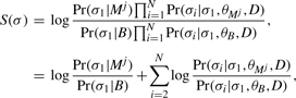(8)

where Pr(σ_i|σ₁,θ,D) is the probability of seeing the letter σ_i in the i-th genome given the symbol σ₁ in the target, given evolutionary distance D separating the target from each of the other genomes, and given the evolutionary model θ. (Note that the first term in Equation (8) is just the PWM score of the position in target genome.)

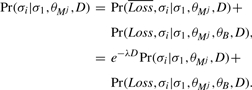
We compute the probability under the background evolutionary model, Pr(σ_i|σ₁, θ_B, D), using the ‘pruning algorithm’ of Felsenstein (1981). The same is true for evolution under the motif model, Pr(σ_i|σ₁, θ_M, D), when we do not allow site loss. When sites can be lost, however, this probability is the sum of two cases—either there is no site loss event, or there is exactly one. Letting Loss be a Boolean variable indicating whether such an event occurs, we can rewrite the probability as

(9)

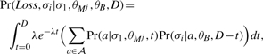
The first term in the sum in Equation (9) is the probability of no loss event [1−F(D), Equation (7)] times the probability under the no-loss model, which can be computed using the pruning algorithm. The second term in the sum in Equation (9), Pr(σ_i, Loss|σ₁, θ_M^j, θ_B, D), is the probability that a loss occurred sometime over the period D and symbol σ_i in the i-th genome ‘evolved’ from residue σ₁ in the target genome given that prior to the loss it evolved according to the motif model, k θ_M, and after the loss event it evolved according to the background model, θ_B. This term can be computed by integrating over all times, t, where the loss event might have occurred, and over all symbols, a, that might have been present at the time of the loss,

(10)

where 𝒜 is the DNA alphabet. To compute Equation (10), we numerically approximate the integral using the rectangle method with the midpoint rule, computing each of the probabilities using the pruning algorithm. We validated the effectiveness of this approach by empirically generating multiple alignments in which motif sites were lost with a frequency determined by our exponential loss function. The numerical approximations produced probabilities correct to three decimal places.

2.6 Estimating the number of TFBSs in a genome

One way to estimate the number of binding sites in a genome is to choose the smallest number of sites such that our theoretical model of PMM score distributions predicts a higher (better) sensitivity (number of predictions) at all q-values than we observe when measuring empirical accuracy using column-shuffled motifs. This is motivated by the assumption that the theoretical model provides an (estimated) upper bound on prediction accuracy, so the empirical accuracy estimates should not exceed the theoretical accuracy estimates. As described in Section 3.4, we find that the requirement that the theoretical sensitivity be higher at all q-values is too strict. Therefore, we instead estimate the smallest number of sites such that the requirement is met on the q-value interval [0, Q]. We study the behavior of this estimate as we vary Q.

To compute our estimate of the true number of binding sites, b, for a given TF, we first use the shuffled-motif method to compute empirical estimates of, for each observed score, s, the q-value of the score, Q_E(s) and the observed number of predictions with that score or better, C_E(s). We then use our theoretical model of PMM score distributions to compute the equivalent (theoretical) values Q_T(s, b) and C_T(s, b), each of which depends on an assumed number of true binding sites, b. To describe our requirement that the theoretical accuracy always be better than the empirical at all q-values, we need to define functions that map q-values to scores. Because more than one score may have the same q-value, we define the inverse functions as the minimum score with a given q-value,

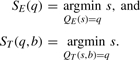Finally, we search for the minimum value of b, , such that the requirement that the observed number of predictions, C_E(s), is always less than the expected number of predictions under the theoretical model, C_T(s, b) for all values of q in the range [0, Q],

(11)

For each value of Q, gives an estimate of the true number of sites.

In order to get our theoretical estimates of the q-values and numbers of predictions at different scores, we proceed as follows. Given that there are b true binding sites and n−b non-binding sites, we expect that there will be TP(s, b)=bP_M(s) true positive predictions and FP(s, b)=(n−b)P_B(s) false positive predictions at a score threshold of s, where P_M(s) and P_B(s) are as defined in Equations (5) and (6), respectively. The expected theoretical FDR of score s is the proportion of false positive predictions:

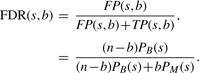Plugging this estimate of FDR into Equation (4) gives us Q_T(s, b), our theoretical score to q-value mapping function. The theoretical score to number of predictions map is just the sum of the numbers of true and false positives, C_T(s, b) = TP(s,b)+FP(s,b).

For comparison, we apply a previously described statistical technique which assumes that the observed score distribution is a mixture of two distinct distributions. One distribution characterizes the real sites (alternative distribution), and the other characterizes the background sites (null distribution). The values π₀ and π₁ are defined as the fraction of scores drawn according to the null and alternative distributions, respectively. To estimate these two values, we use an implementation of the bootstrapping method described by Storey (2002). This method selects an optimal P-value threshold, , and then estimates π₀ as

where n is the total number of P-values. Using this approach, the estimate of the number of real sites is

3 RESULTS AND DISCUSSION

3.1 PMM scanners perform worse than a simple PWM scan at predicting known TFBSs

We first show that using a gold standard of known yeast TFBSs in a cross-validated experiment indicates that there is no advantage in prediction accuracy with PMM scanners compared with a standard PWM scan. Actually, the opposite appears true, as shown in Table 1. At a sensitivity level of 50%—when half of the known binding sites are detected—the simple PWM scan has better accuracy (lower cross-validated FDR) than all three PMM scanners tested for 14 out of the 21 TF motifs. The apparent superiority of simple PWM scanning persists over all sensitivity levels (data not shown).

Table 1.

Evaluation of PWM and PMM scanners using a gold standard

TF name	False discovery rate at 50% sensitivity
	PWM	Motiph	Monkey	rMonkey
ABF1	76.6	069.2a	70.2	71.3
BAS1	88.2	76.2	51.6a	55.9
GAL4	0.0a	31.5	29.6	24.2
GCN4	76.5a	84.8	80.8	79.0
HAP1	75.0a	94.3	96.2	94.6
HSE,HSTF	63.2a	82.3	69.9	71.7
MATalpha2	68.1a	95.1	98.7	97.0
MCM1	31.8a	83.0	75.4	78.6
MIG1	85.5a	99.4	99.5	99.5
PDR1	0.0a	55.4	99.2	98.7
PHO4	81.7a	87.5	90.6	89.3
RAP1	55.9a	91.8	86.9	58.8
REB1	94.1	91.1	88.5	88.2a
repressor_of_CAR1	90.4a	97.7	97.8	97.1
ROX1	86.6	20.0b	20.0b	20.0b
SWI5	89.4a	95.9	92.1	89.9
TBP	99.0	96.8	96.3	95.2a
UASH	99.0a	100.0	99.9	99.6
UASPHR	99.9	100.0	99.9	99.3a
UIS	72.7a	83.3	89.0	89.1
URS1H	29.0	25.0a	40.0	40.0
Wins	14	2	1	3
Ties	0	1	1	1

The cross-validated FDR (%) at a sensitivity of 50% of a simple PWM scanner and three different PMM scanning algorithms evaluated on a gold standard set of yeast TFBSs is shown. Column headings give the name of the program. All PMM-based scans use the HKY+HB evolutionary model. Each row gives FDR when predicting the gold standard sites of the named TF.

^aThe best for values (lowest) in their row.

^bValues tied for the best FDR. Total number of wins and ties for each method is shown at bottom.

The differences in accuracy are often substantial. For one TF (PDR1), the PWM scan of just the S.cerevisiae genome achieves a 0% FDR, while the three PMM algorithms, which scan multiple alignments of four yeast genomes, have false discovery rates of at least 55% and up to 99%. In the few cases where the simple PWM scan does not outperform the other methods, its FDR is often quite close to that of the other algorithms. The one exception is the TF ROX1, where the phylogenetic algorithms achieve much lower FDR than the single sequence scan (20% versus 87%). In general, however, this experiment fails to demonstrate any substantial benefit to using phylogenetic motif scanning.

Several explanations are possible for the apparent failure of the phylogenetic motif scanners in this test. Errors in the multiple alignments of the intergenic regions could be causing conserved sites to receive poor scores. This explanation is supported by the observation that the rMonkey algorithm, which performs extensive re-alignment of the sequences during scanning, does slightly better than Motiph, which simply ignores gapped regions. Re-alignment strategies used by Monkey and rMonkey can also recover sites that have ‘drifted’–the original site is not conserved but a new site has emerged nearby. Both algorithms restrict re-alignments to very narrow windows, however, and neither can correct for sites that have drifted to the opposite strand. These limitations may partially explain the fact that Monkey and rMonkey do not perform substantially better than Motiph, which has no re-alignment strategy. (Careful examination of Table 1 shows that Motiph has lower FDR than both Monkey and rMonkey in 8 out of 21 cases.)

An alternative explanation for the apparent failure of the phylogenetic motif scanners is that errors within the gold standard are systematically biased against phylogenetic-based scanning. We expect that the gold standard is missing some, and possibly many, functional sites. These missing sites will be flagged as false positives, and can cause an algorithm that correctly detects them to have a larger (apparent) FDR. The sites missing from the gold standard are likely to be minor variants of the motif with slightly lower binding affinity, such that the experimental methods for identifying protein to DNA binding sites overlook them. If these sites are nevertheless highly conserved, then the phylogenetic scanners will score them much higher and appear to have a larger number of false positive predictions. This effect may be contributing to the apparent failure of the phylogenetic motif scanners to improve upon single sequence scanning. We provide evidence for this hypothesis in the next section.

3.2 PMM scanners are more accurate than PWM scanners

When we measure prediction accuracy without reference to gold standard sets of known sites, it becomes clear that PMM scanners are more accurate than simple PWM scans. The q-value (minimum FDR) of each of the scanners, estimated using the column-shuffled motif approach, is shown for the yeast TF motifs in Table 2. The table gives the prediction accuracy at two different levels of sensitivity— 20 and 50 total predicted sites. When making 50 binding site predictions, PMM scans have lower minimum FDR than PWM scans with 16 of the 21 yeast TF motifs used in this study. When 20 binding sites are predicted, PMM scans have lower minimum FDR for 17 out of 21 motifs. The improvement over the simple PWM scan of each of the PMM scanners is statistically significant according to a signed rank test (Motiph, p=0.013; Monkey, p=0.001; and rMonkey, p=0.008).

Table 2.

Evaluation of PWM and PMM scanners using a shuffled-motif control

TF name	q-value (min FDR) at 20 predictions				q-value (min FDR) at 50 predictions
	PWM	Motiph	Monkey	rMonkey	PWM	Motiph	Monkey	rMonkey
ABF1	20.1	19.5	7.4a	12.4	61.9	43.7	33.6a	37.8
BAS1	71.0	72.5	34.8a	35.0	92.8	75.7a	75.9	80.1
GAL4	60.4a	94.4	69.0	85.9	97.7	95.3	88.5a	97.2
GCN4	59.1	13.4a	19.6	26.2	78.1	51.5a	61.6	71.5
HAP1	66.5	27.7a	32.8	41.5	66.5	47.5	34.8a	46.1
HSE,HSTF	27.6	17.7a	29.0	25.5	42.9a	46.9	64.0	62.2
MATalpha2	75.7	58.1	53.4a	56.9	77.0	63.9	62.6a	66.2
MCM1	11.4a	22.1	25.5	19.5	30.8a	51.2	60.9	66.2
MIG1	43.5	35.0	25.8a	31.9	57.7	64.7	54.7a	60.1
PDR1	27.2a	31.8	61.1	58.9	41.2	33.9a	61.1	58.9
PHO4	41.5	25.5	18.3a	27.0	56.8	45.8	39.0a	46.7
RAP1	16.5a	30.0	27.5	21.0	48.9a	64.2	52.3	49.2
REB1	48.7	10.9	7.3a	9.0	48.7	24.9	17.7a	23.1
repressor_of_CAR1	20.5	10.7	8.0	7.7a	45.5a	57.0	55.5	57.8
ROX1	63.9	64.9	40.4a	48.5	79.3	67.3	60.2	54.6a
SWI5	72.8	76.0	64.0a	75.7	81.3	76.0	64.0a	75.7
TBP	13.3	0.0b	0.0b	6.8	13.3a	22.1	17.8	20.2
UASH	77.8	79.2	73.8a	73.9	79.4	79.2	77.1	73.9a
UASPHR	59.0	47.7a	64.0	50.5	70.8	70.2a	79.7	71.8
UIS	51.4	50.0	31.5a	45.0	73.0	70.6	54.4a	56.5
URS1H	3.2	7.0	1.0a	1.4	53.4	41.2	27.6a	31.3
Wins	4	4	11	1	5	4	10	2
Ties	0	1	1	0	0	0	0	0

The estimated q-value (minFDR %) of a simple PWM scanner and three different PMM scanning algorithms. Column headings give the name of the program. All PMM-based scans use the HKY+HB evolutionary model. Each row gives q-value (minFDR) estimated using shuffled motifs to estimate the null score distribution.

^a The best q-values in their row.

^bValues tied for the best q-value. Total number of wins and ties for each method at the given number of predictions is shown at bottom.

The systematic improvement of all phylogenetic motif scanners over the PWM scanner strongly supports the hypothesis that the gold standard data are systematically biased against the phylogenetic motif scanners. Therefore, these results suggest that not only do all of the models perform better than the gold standard indicates, but in many cases the PMMs provide a considerable advantage over PWM scanning.

The results in Table 2 also indicate that the different realignment strategies used by the three PMM scanners make a large difference. The approach used by the Monkey algorithm works best with the 21 yeast TF motifs studied here. Monkey has the best accuracy among all the prediction algorithms for 11 out of the 21 motifs at a sensitivity level of 20 predictions, and for 10 motifs at a sensitivity level of 50 predictions.

3.3 Incorporating site loss improves our theoretical estimate of the statistical power of PMM scanners

The extension of our earlier model of the statistical power of PMM scanners to allow loss-of-site events causes it to agree more closely with the observed power of PMM scanners on the yeast gold standard TFBS sets. We evaluate the accuracy of the theoretical model by comparing the ROC curves (Swets, 1988) it predicts with the ROC curves generated by our cross-validation experiments with the 21 yeast TF motifs. An example of the behavior of the theoretical model under five different assumptions of the probability of site loss events, ranging from no loss to up to 51% chance of loss in any lineage, is shown in Figure 1. Assuming 51% chance of loss shifts the theoretical ROC curve about an order of magnitude closer to the observed ROC curve. This plot is typical of the plots for all 21 TF motifs (data not shown).

Fig. 1.

Theoretical and empirical ROC curves for the ABF1 motif. The empirical ROC curves are shown as points, and are the results of the cross-validation experiment using the gold standard binding site set for ABF1. The theoretical curves are shown for different choices of the loss rate parameter, λ, and the corresponding percentage chance of a loss in any lineage is indicated.

The extended theoretical model also agrees well with empirical estimates of statistical power based on the shuffled-motif approach. Figure 2 shows that, if we assume that there are 51 real ABF1 binding cites in the yeast intergenic regions, the theoretical estimate of the statistical power of PMM scanning fits the empirical results using the Monkey scanning algorithm quite closely, except for very high q-values (low search specificity).

Fig. 2.

Theoretical and empirical statistical power curves for the ABF1 motif. The empirical curve (points) is computed using the shuffled-motif approach with the Monkey PMM scanning algorithm. The two theoretical curves are generated using the theoretical model with 51% chance of loss on any lineage and with the given estimates of the numbers of real sites (shown in parentheses).

In the extreme case where the probability of loss is 51%, the total probability that any particular site is conserved over all three comparative genomes (assuming independence) is equal to 12.5%. This value acts as a reasonable upper bound on the expected amount of site loss we would expect in this study, because estimates of the rate at which binding sites are perfectly conserved across three yeast genomes vary from 13% to 20% (Borneman et al., 2007; Tuch et al., 2008).

3.4 Estimating the number of TFBSs in yeast

Our procedure for predicting the number of real binding sites in S.cerevisiae results in estimates that are realistic, and in much greater agreement with the SCPD database than the estimates produced using the bootstrapping method, as shown in Table 3. We fit our theoretical model with individual site loss occuring at a probability of 51% to the empirical data. Our model-based procedure finds the minimum number of sites such that the theoretical model expects more predictions than we observe according to the empirical, for all q-values up to the threshold Q. The alternative method, called bootstrapping, uses P-values estimated using the shuffled-motif approach. The complete list of P-values for all positions scanned within the genome is used to estimate the proportion, π₁, of the P-values that do not belong to the null distribution, hence the number of real binding sites (Storey, 2002) (Section 2.6). We ran the bootstrapping method, with 10 000 bootstraps, 100 times, and we report the mean and SD of the estimate of true binding sites.

Table 3.

Estimated number of real binding sites for 21 yeast TFs

TF Name	SCPD	Model-based	Bootstrapping
	No. of sites	No. of sites	No. of sites	(SD)
ABF1	16	51	175	(62)
BAS1	5	15	117	(0)
GAL4	10	9	49770	(956)
GCN4	10	47	62587	(1957)
HAP1	5	44	56753	(2892)
HSE,HSTF	7	34	131	(0)
MATalpha2	12	20	0	(0)
MCM1	34	40	0	(0)
MIG1	9	37	739	(23)
PDR1	11	4	36	(0)
PHO4	8	36	1091	(82)
RAP1	16	24	42434	(1967)
REB1	17	105	59299	(709)
repressor_of_CAR1	12	42	51189	(990)
ROX1	8	18	46	(0)
SWI5	6	5	133	(0)
TBP	10	118	427	(8)
UASH	14	14	145	(31)
UASPHR	15	25	93	(9)
UIS	5	21	1144	(127)
URS1H	13	48	176	(46)

The estimated number of real binding sites compared with the numbers present in SCPD. Two methods are used to produce the estimates: the bootstrapping method (Storey, 2002) and our model-based method that chooses the number of sites that insures that the theoretical statistical power of the scan is an upper bound on the empirical power. For our model-based method, we report .

The plot in Figure 3 illustrates the results of our model-based method with a typical example of the relationship between the q-value threshold, Q, and number of predicted real sites, , for the motif ABF1. We include in the plot the results for the theoretical model with and without binding site loss. In the plot allowing binding site loss, we have calibrated the parameters of the loss model to emulate the most pessimistic estimate in the literature (Tuch et al., 2008), such that a site has 51% probability of being lost on an individual branch of the tree. We observe that, for all motifs, the estimated number of sites undergoes a phase transition at high q-values. Up to some value of Q, the no-loss estimate tends upwards on a slight slope. However, when we use the loss model, the estimate remains much flatter throughout the first two-thirds of the plot. We also observe that, for all motifs, the estimated number of sites at a q-value threshold of 0.5 is stable across a considerable range of q-values (data not shown). To produce a final estimate of the number of real binding sites, shown in Table 3, we found the minimum number of real binding sites for which the theoretical loss model dominated the empirical results up to a q-value of Q=0.5. The flatness of the plot using the site loss model demonstrates that the theoretical data fit the empirical data best using an approximately constant estimate of the number of binding sites, indicating that it is a better model of binding site evolution.

Fig. 3.

Effect of different values of Q on the model-based estimate of the number of real sites for the ABF1 motif. The curves show our model-based estimates, , of the number of real binding sites for the ABF1 motif, as a function of Q Equation (11). The model-based estimates are based on scans using the Monkey algorithm, and two different values of the theoretical loss rate parameter, corresponding to 0% and 50% loss in any lineage.

4 CONCLUSION

We have demonstrated that measuring the accuracy of binding site predictors using collections of known sites may be dangerously misleading because such collections may be missing ‘weak’ sites, which are exactly the type of sites needed to discriminate among predictors. When we abandon the gold standard and consider the number of statistically significant sites predicted, using column-shuffled ‘random’ motifs to measure significance, the PMM scanners perform much better than the PWM.

Due to the assumptions embedded in the development of any null model, we cannot be certain that the relative performance statistics reported in this work are a perfect reflection of the prediction on the true set of binding sites. Nevertheless, the observation that all PMMs perform similarly and with statistically significant improvement over the PWM suggests that the results are not an aberration. Among the three scanning algorithms that we test, the MONKEY algorithm has the highest accuracy for predicting yeast TFBSs.

We also introduce a novel theoretical model of binding site evolution that includes loss-of-site events. This model provides a better fit to the observed empirical performance than our original theoretical model of PMM statistical power (Hawkins and Bailey, 2008).

Statistical algorithms for estimating the proportion of samples that do not belong to the null distribution are of immense importance in data mining. However, our experiments with the bootstrapping procedure suggest that this method is unreliable for small values of π₁. We implement an alternative approach to estimating the number of binding sites that makes use of an explicit theoretical model of the expected performance of the predictor. The results we produce using this procedure conform to our expectations and appear to be a reasonable estimate of the number of true binding sites within the yeast genome, and are in most cases several multiples of the number of known sites listed in the SCPD.

REFERENCES

- Berman BP, et al. Exploiting transcription factor binding site clustering to identify cis-regulatory modules involved in pattern formation in the Drosophila genome. Proc. Natl Acad. Sci. USA. 2002;99:757–762. doi: 10.1073/pnas.231608898. [DOI] [PMC free article] [PubMed] [Google Scholar]
- Blanchette M, et al. Aligning multiple genomic sequences with the threaded blockset aligner. Genome Res. 2004;14:708–715. doi: 10.1101/gr.1933104. [DOI] [PMC free article] [PubMed] [Google Scholar]
- Boffelli D, et al. Phylogenetic shadowing of primate sequences to find functional regions of the human genome. Science. 2003;299:1391–1394. doi: 10.1126/science.1081331. [DOI] [PubMed] [Google Scholar]
- Borneman AR, et al. Divergence of transcription factor binding sites across related yeast species. Science. 2007;317:815–819. doi: 10.1126/science.1140748. [DOI] [PubMed] [Google Scholar]
- Brudno M, et al. Lagan and multi-lagan: efficient tools for large-scale multiple alignment of genomic DNA. Genome Res. 2003;13:721–731. doi: 10.1101/gr.926603. [DOI] [PMC free article] [PubMed] [Google Scholar]
- Chenna R, et al. Multiple sequence alignment with the clustal series of programs. Nucleic Acids Res. 2003;31:3497–3500. doi: 10.1093/nar/gkg500. [DOI] [PMC free article] [PubMed] [Google Scholar]
- Doniger SW, Fay JC. Frequent gain and loss of functional transcription factor binding sites. PLoS Comput. Biol. 2007;3:e99. doi: 10.1371/journal.pcbi.0030099. [DOI] [PMC free article] [PubMed] [Google Scholar]
- Eddy SR. A model of the statistical power of comparative genome sequence analysis. PLoS Biol. 2005;3:e10. doi: 10.1371/journal.pbio.0030010. [DOI] [PMC free article] [PubMed] [Google Scholar]
- Felsenstein J. Evolutionary trees from DNA sequences: a maximum likelihood approach. J. Mol. Evol. 1981;17:368–376. doi: 10.1007/BF01734359. [DOI] [PubMed] [Google Scholar]
- Gertz J. Analysis of combinatorial cis-regulation in synthetic and genomic promoters. Nature. 2008;457:215–218. doi: 10.1038/nature07521. [DOI] [PMC free article] [PubMed] [Google Scholar]
- Guccione E. Myc-binding-site recognition in the human genome is determined by chromatin context. Nat. Cell Biol. 2006;8:764–U225. doi: 10.1038/ncb1434. [DOI] [PubMed] [Google Scholar]
- GuhaThakurta D. Computational identification of transcriptional regulatory elements in DNA sequence. Nucleic Acids Res. 2006;34:3585–3598. doi: 10.1093/nar/gkl372. [DOI] [PMC free article] [PubMed] [Google Scholar]
- Gumucio DL, et al. Phylogenetic footprinting reveals a nuclear protein which binds to silencer sequences in the human gamma and epsilon globin genes. Mol. Cell Biol. 1992;12:4919–4929. doi: 10.1128/mcb.12.11.4919. [DOI] [PMC free article] [PubMed] [Google Scholar]
- Halpern AL, Bruno WJ. Evolutionary distances for protein-coding sequences: modeling site-specific residue frequencies. Mol. Biol. Evol. 1998;15:910–917. doi: 10.1093/oxfordjournals.molbev.a025995. [DOI] [PubMed] [Google Scholar]
- Hasegawa M, et al. Dating of the human-ape splitting by a molecular clock of mitochondrial DNA. J. Mol. Evol. 1985;22:160–174. doi: 10.1007/BF02101694. [DOI] [PubMed] [Google Scholar]
- Hawkins JC, Bailey TL. The statistical power of phylogenetic motif models. In: Vingron M, Wong L, editors. 12th Annual International Conference on Computational Biology. Springer; 2008. pp. 112–126. RECOMB 2008. [Google Scholar]
- Katoh K, et al. Mafft: a novel method for rapid multiple sequence alignment based on fast fourier transform. Nucleic Acids Res. 2002;30:3059–3066. doi: 10.1093/nar/gkf436. [DOI] [PMC free article] [PubMed] [Google Scholar]
- Kellis M, et al. Sequencing and comparison of yeast species to identify genes and regulatory elements. Nature. 2003;423:241–254. doi: 10.1038/nature01644. [DOI] [PubMed] [Google Scholar]
- Kheradpour P, et al. Reliable prediction of regulator targets using 12 Drosophila genomes. Genome Res. 2007;17:1919–1931. doi: 10.1101/gr.7090407. [DOI] [PMC free article] [PubMed] [Google Scholar]
- Kouzarides T. Chromatin modifications and their function. Cell. 2007;128:693–705. doi: 10.1016/j.cell.2007.02.005. [DOI] [PubMed] [Google Scholar]
- Levine M, Tjian R. Transcription regulation and animal diversity. Nature. 2003;424:147–151. doi: 10.1038/nature01763. [DOI] [PubMed] [Google Scholar]
- Liu X. Whole-genome comparison of Leu3 binding in vitro and in vivo reveals the importance of nucleosome occupancy in target site selection. Genome Res. 2006;16:1517–1528. doi: 10.1101/gr.5655606. [DOI] [PMC free article] [PubMed] [Google Scholar]
- Moses AM, et al. MONKEY: identifying conserved transcription-factor binding sites in multiple alignments using a binding site-specific evolutionary model. Genome Biol. 2004;5:R98. doi: 10.1186/gb-2004-5-12-r98. [DOI] [PMC free article] [PubMed] [Google Scholar]
- Moses AM, et al. Large-scale turnover of functional transcription factor binding sites in drosophila. PLoS Comput. Biol. 2006;2:e130. doi: 10.1371/journal.pcbi.0020130. [DOI] [PMC free article] [PubMed] [Google Scholar]
- Narlikar L, et al. A nucleosome-guided map of transcription factor binding sites in yeast. PLos Comput. Biol. 2007;3:e215. doi: 10.1371/journal.pcbi.0030215. [DOI] [PMC free article] [PubMed] [Google Scholar]
- Staden R. Searching for patterns in protein and nucleic acid sequences. Methods Enzymol. 1990;183:193–211. doi: 10.1016/0076-6879(90)83014-z. [DOI] [PubMed] [Google Scholar]
- Storey JD. A direct approach to false discovery rates. 2002 [Google Scholar]
- Stormo GD. DNA binding sites: representation and discovery. Bioinformatics. 2000;16:16–23. doi: 10.1093/bioinformatics/16.1.16. [DOI] [PubMed] [Google Scholar]
- Swets JA. Measuring the accuracy of diagnostic systems. Science. 1988;240:1285–1293. doi: 10.1126/science.3287615. [DOI] [PubMed] [Google Scholar]
- Tuch BB, et al. The evolution of combinatorial gene regulation in fungi. PLoS Biol. 2008;6:e38. doi: 10.1371/journal.pbio.0060038. [DOI] [PMC free article] [PubMed] [Google Scholar]
- Wasserman WW, Sandelin A. Applied bioinformatics for the identification of regulatory elements. Nat. Rev. Genet. 2004;5:276–287. doi: 10.1038/nrg1315. [DOI] [PubMed] [Google Scholar]
- Whitington T, et al. High-throughput chromatin information enables accurate tissue-specific prediction of transcription factor binding sites. Nucleic Acids Res. 2008;37:14–25. doi: 10.1093/nar/gkn866. [DOI] [PMC free article] [PubMed] [Google Scholar]
- Zhu J, Zhang MQ. SCPD: a promoter database of the yeast Saccharomyces cerevisiae. Bioinformatics. 1999;15:607–611. doi: 10.1093/bioinformatics/15.7.607. [DOI] [PubMed] [Google Scholar]