Prediction of sub-cavity binding preferences using an adaptive physicochemical structure representation

Abstract

Motivation: The ability to predict binding profiles for an arbitrary protein can significantly improve the areas of drug discovery, lead optimization and protein function prediction. At present, there are no successful algorithms capable of predicting binding profiles for novel proteins. Existing methods typically rely on manually curated templates or entire active site comparison. Consequently, they perform best when analyzing proteins sharing significant structural similarity with known proteins (i.e. proteins resulting from divergent evolution). These methods fall short when used to characterize the binding profile of a novel active site or one for which a template is not available. In contrast to previous approaches, our method characterizes the binding preferences of sub-cavities within the active site by exploiting a large set of known protein–ligand complexes. The uniqueness of our approach lies not only in the consideration of sub-cavities, but also in the more complete structural representation of these sub-cavities, their parametrization and the method by which they are compared. By only requiring local structural similarity, we are able to leverage previously unused structural information and perform binding inference for proteins that do not share significant structural similarity with known systems.

Results: Our algorithm demonstrates the ability to accurately cluster similar sub-cavities and to predict binding patterns across a diverse set of protein–ligand complexes. When applied to two high-profile drug targets, our algorithm successfully generates a binding profile that is consistent with known inhibitors. The results suggest that our algorithm should be useful in structure-based drug discovery and lead optimization.

Contact: izharw@cs.toronto.edu; lilien@cs.toronto.edu

1 INTRODUCTION

The ability to identify and exploit patterns of protein–small-molecule interaction is a critical component of protein function prediction, pharmacophore inference, molecular docking and protein design (Halperin et al., 2002; Langer and Hoffmann, 2006; Powers et al., 2006; Sousa et al., 2006). In most cases, the protein–ligand interface is characterized by a number of geometric and/or chemical features (Dror et al., 2006). This characterization is facilitated by mining high-resolution experimental structures where, ideally, a single protein would be observed interacting with several different bound ligands. Unfortunately, for most proteins, this type of multiple-binding information is not available (Berman et al., 2000). To avoid this problem, we chose to focus on sub-cavities within an active site with the assumption that structurally similar sub-cavities are likely to exhibit similar binding profiles. It is important to emphasize the definition of sub-cavity utilized in this work. We define a sub-cavity to be a small region of the traditionally described active site capable of interacting with a single chemical group (e.g. phenyl, hydroxyl and carboxyl). That is, an active site is generally composed of 5–20 sub-cavities. By considering protein–ligand interactions at the sub-cavity level, we can utilize binding information from structurally and functionally distinct proteins. A pair of proteins whose active sites differ significantly when compared in their entirety may still share similarity at the sub-cavity level. In this work, we decompose a target active site into a set of sub-cavities, identify structurally similar sub-cavities within other proteins and then use this information to construct a binding profile. This approach enables inference when no global receptor similarity is available.

There are several existing approaches to analyzing an active site's protein–ligand binding preference. In most cases, these methods aim to predict protein function which differs from our aim of identifying the local binding patterns of sub-cavities. A result of these different goals is that a direct comparison between our work and the described methods using a common dataset is not feasible. State-of-the-art methods can be classified into three groups:

Template-based methods: these methods (Laskowski et al., 2005; Stark and Russell, 2003; Wallace et al., 1997) accept a template structure as input (e.g. catalytic triad in serine proteases) and query a given structural database for matching patterns. Their reliance on the provided input template makes them particularly useful for studying or predicting relations to an already known pattern. The strength of the template-based methods is their speed. The lightweight template representation (usually, a set of amino acid residues) allows rapid queries against large databases; however, the templates are often overly simplistic and are incapable of capturing the rich physicochemical variations among binding pockets. Further, templates are often manually generated and are therefore restricted in their complexity. These limitations make general binding site analysis with template-based methods difficult.

Binding site similarity methods: these methods compare entire binding sites and retrieve sets of proteins which share globally similar binding patterns. They are commonly used for protein function prediction where similar binding patterns imply similar catalytic functionality. Several approaches utilize active site geometry (i.e. amino acid backbone, solvent accessible surface or active site volume) (Kuhn et al., 2006; Morris et al., 2005), while other methods exploit both geometry and the chemical function of the amino acid residues flanking the binding site (Najmanovich et al., 2008; Schmitt et al., 2002; Shatsky et al., 2005). A slightly different approach combines sequence alignment with subsequent spatial pattern matching of the defined active site surface (Binkowski et al., 2003). These methods infer patterns using a variety of techniques to identify similarity such as sub-graph isomorphism, geometric hashing, multiple structural alignment and clique detection (Kinoshita and Nakamura, 2003; Leibowitz et al., 2001; Pennec and Ayache, 1998; Shulman-Peleg et al., 2008). Unlike the template-based methods, the binding site similarity methods often utilize an elaborate model that includes both geometrical constraints and chemical profile. While these methods are suitable for comparing whole binding sites, they are less effective when considering functionally similar proteins which only share local ‘hot-spots’ within their binding pockets. They are also less useful when analyzing proteins with novel structure and function. These novel proteins are unlikely to match any patterns derived from known active sites.

Local binding site similarity methods: recently methods that search for local similarities within binding sites have emerged. These methods allow inference when global active site similarity is poor. They characterize local interaction patterns within the binding site cavity. The latter is particularly useful for structure-based drug discovery, where the interaction between a ligand's chemical group and the flanking amino acids can be separately studied outside the context of the binding site. In (Kupas et al., 2007), the Klebe group defines a set of functional pseudo-centers for each amino acid and pairs each pseudo-center with an associated surface-patch (Schmitt et al., 2002). Each surface-patch reflects the chemical function and location of its corresponding residue. A wavelet representation of the surface-patches allows fast structural comparison with adjustable resolution. A slightly different approach (Ramensky et al., 2007) associates each sub-cavity with its occupying ligand fragment. Using the ligand fragments as anchor points, the sub-cavities are aligned and a similarity is computed using the spatial and chemical overlap of the neighboring residues. Local similarity methods suffer from two major shortcomings. First, existing methods define sub-cavities using an arbitrary fixed distance threshold from either the associated residue or the ligand fragment. Second, the inclusion of apo proteins potentially reduces the quality of identified templates. Selecting a threshold that is too large results in the inclusion of irrelevant and potentially confusing residues. Conversely, a threshold that is too small results in a partial model that ignores relevant residues; proteins frequently undergo moderate structural changes upon ligand binding. Methods which ignore the holo structure are likely to infer a biased view of the binding profile.

2 APPROACH

We have developed a sub-cavity-based approach to characterizing protein–small-molecule binding patterns. Our algorithm deconstructs the active site into a set of potentially overlapping sub-cavities and then infers the binding profile of each sub-cavity. The deconstruction allows us to exploit the sub-cavity similarity that often exists between structurally diverse proteins. The binding profile of the entire active site can then be constructed by joining the information gleaned from each sub-cavity. The approach differs from previous work in several important ways: first, we analyze only protein–small-molecule complexes. The current abundance and diversity of holo structures allows us to avoid inclusion of apo structures during learning. This design decision removes binding site localization from the inference problem and ensures that analyzed sub-cavities are indeed involved in binding. We discuss the possibility of relaxing this restriction in Section 4.4. Second, we divide each binding site into sub-cavities according to the chemical groups of the bound ligand. This separation enables us to identify sub-cavities that are likely to form interactions, and more importantly, to label each sub-cavity with the chemical group to which it is bound (i.e. its functionality). Third, we model sub-cavities by combining the shape of the binding site (i.e. its solid 3D volume) with the chemical profile of its flanking residues to form a single physicochemical representation. This allows us to benefit from the accuracy of modeling the shape of the active site while still accounting for the chemical properties of the surrounding residues. Furthermore, this representation allows us not only to avoid matching the flanking residues directly but also to account for their cumulative effects at any location within the sub-cavity. Finally, we allow the algorithm to iteratively cluster sub-cavities with the same function and to reshape sub-cavities. The iterative sub-cavity reshaping procedure is unique to our approach and provides an advantage over simply including all residues within a distance cutoff. Reshaping increases the within-class similarity (i.e. sub-cavities with the same function become more similar) while reducing the between-class similarity. This procedure not only improves the classification results (Section 4) but also produces optimized sub-cavity structures.

In the context of this article, we define the following terms: (i) a chemical group is a group of atoms that characterize a chemical moiety. Like a set of building blocks, a limited set of chemical groups can specify the structure of virtually all small molecules. We utilize a set of 47 chemical groups (e.g. phenyl, hydroxyl, carboxyl) inspired by (Chen et al., 1999). (ii) A function type is the mapping of a chemical group to its corresponding chemical interaction type. We utilize six functional types: hydrophobic, aromatic, acid, base, hydrogen-bond donor (HBD) and hydrogen-bond acceptor (HBA) (McGregor, 2007). Because some chemical groups correspond to more than one function type (i.e. HBD and HBA) the mapping is one-to-many. In practice, each of our 47 chemical groups can be described by one of only 9 sets of function types.

In this framework, a small molecule can be considered a spatial arrangement of active chemical groups connected by inert bridging fragments. We propose that within a sub-cavity, the function types of the protein residues specify a set of preferred ligand fragments (i.e. chemical groups) with which to bind. Recent analysis of the binding site variations (Kahraman et al., 2007) as well as local binding site similarity methods (Kupas et al., 2007; Ramensky et al., 2007) provide evidence that such patterns do exist. Using the structures of solved protein complexes we can learn which sub-cavities (parametrized by shape and function type) preferentially associate with which ligand fragments (parametrized by chemical group). Using the occupying ligand fragments to define sub-cavities not only isolates properly configured sub-cavities but also pairs each sub-cavity with the bound chemical group. This information can then be used to infer a binding profile for a query potentially apo protein.

3 METHODS

The training of our algorithm can be divided into a sub-cavity generation stage (steps 1–4) and a sub-cavity comparison stage (steps 5–6). The process is summarized below and in Figure 1.

1. Dataset generation: (Section 3.1) generate a non-redundant set of protein–small-molecule complexes.

2. Ligand chemical analysis: (Section 3.2) identify the chemical groups of each bound ligand.

3. Shape identification and characterization of binding sites: Section (3.3) generate a 3D model of the binding site bounded by the solvent accessible surface. Assign the function types (Section 2) for each point in the volume based on the flanking residues.

4. Binding site division into sub-cavities: (Section 3.2) divide the model into sub-cavities corresponding to the identified chemical groups of the bound ligand.

5. Sub-cavity clustering: (Sections 3.5 and 3.6) compute the pairwise similarity of all sub-cavities and cluster.

6. Sub-cavity reshaping: (Section 3.6) identify outliers within each cluster (i.e. sub-cavities binding a ligand chemical group that is different than the plurality of sub-cavities in the cluster) and structurally reshape the inliers to increase their similarity.

After generating and clustering the sub-cavities (steps 1–6), we can perform functional inference on a novel sub-cavity with unknown function by assigning the sub-cavity the function type of its most similar cluster.

Fig. 1.

The algorithmic framework is divided of two stages: the sub-cavity generation stage where the sub-cavities are initially identified and the sub-cavity comparison stage where sub-cavities are clustered and reshaped.

3.1 Dataset generation

We developed the PSMDB database (Wallach and Lilien, 2009) explicitly to enable non-biased inference of binding patterns. The PSMDB provides sets of protein–small-molecule complexes that are ideally suited for the analysis in the present work. It includes only high-quality crystal structures that contain at least one non-covalently bound ligand. Furthermore, the PSMDB handles structural redundancy at both the protein and ligand levels and thus contains highly similar ligands interacting with different proteins and different ligands interacting with highly similar proteins. In contrast to other small-molecule databases, this feature provides multiple instances of sub-cavity–ligand interactions while reducing the bias toward any single pattern.

3.2 Ligand chemical analysis

The chemical groups contained within each ligand are used as anchoring points to define the sub-cavities. We identify chemical groups by first defining a template library of chemical groups [modeled after (Chen et al., 1999) and encoded using SMARTS patterns (James et al., 2000)] and then matching these templates against each ligand structure. Similar to the pseudo-center approach described in (Schmitt et al., 2002), we assign a location for each identified chemical group and label the group with up to six features (e.g. HBD, HBA,…) corresponding its functional type. This reduced ligand representation captures the functional type and arrangement of each chemical group while removing structural scaffolding that is not likely to form a significant interaction.

3.3 Shape identification and characterization of binding sites

We identify the binding site cavities and generate structural models that include the shape of the cavity and the function type of the amino acid residues that flank it. Since all input structures contain a bound ligand, we are able to easily identify the location of the binding site. We place the protein structure over a grid of 0.75Å (half the length of a carbon–carbon bond) consisting of grid cells with the center of each cell defined as a grid point. We then assign one of three labels (inner volume, binding surface and inner surface) to each grid cell/point. Starting with one of the ligand's atoms, we select the atom's corresponding grid cell and label it as inner volume. We then iterate over the neighboring grid cells. Inspired by the POCKET and SURFNET algorithms (Laskowski, 1995; Levitt and Banaszak, 1992), we define the solvent accessible surface by first checking for van der Waals clashes of protein atoms with a pseudo water molecule located at each grid point. If there is no clash, we mark the grid cell as an inner volume and recursively proceed to its neighbors. When a grid point clashes with a protein atom, we mark the cell as a binding surface cell, tentatively mark all its neighbors that have not yet been explored as inner surface and then backtrack. The inner surface points are either be relabeled to binding surface or inner volume as they or their neighbors are visited. In order to remain within the cavity, we stop and backtrack when a grid point reaches a distance of >5Å from all ligand atoms. We use a burial degree measurement to locate the mouth of the binding pocket (Schmitt et al., 2002). From each inner volume or surface point, we virtually project beams in the 26 canonical directions. The burial degree of a point is the number of beams that hit a binding surface grid point. We found, visually, that a burial degree of 15 is sufficient to identify binding pockets, thus points with a burial degree smaller than 15 are considered outside the binding pocket and are discarded. Once the shape of the binding site is identified, we locate the amino acid residues that flank it. Then, as in the ligand chemical analysis step, we identify the chemical groups of these residues and map each group to its corresponding functional types. A schematic of the general process is illustrated in Figure 2A.

Fig. 2.

A simplified illustration of the physicochemical analysis of a sub-cavity. (A) illustrates the binding site identification described in Section 3.3. Open square, circle and triangle correspond to inner volume, binding surface and inner surface grid points, respectively. Star corresponds to a chemical group of a flanking amino acid residue. The dashed axes represent the principal axes of the sub-cavity. (B) Illustrates the initialization of the sub-cavity similarity maximization stage described in Section 3.5. The sub-cavity is rigidly transformed such that its principle axes are aligned with the x and y axes and its center of mass is at the origin. The cumulative effect of each flanking functional group (illustrated by the shaded regions) is computed for every grid point in the new coordinate frame that overlaps the sub-cavity.

3.4 Binding site division into sub-cavities

Having identified the extent of the binding site as well as the chemical groups of the ligand, we then define sub-cavities that are likely to participate in binding. We define a sub-cavity to be the region of the binding site that surrounds a chemical group of the bound ligand (Fig. 5) and we label the sub-cavity with the chemical group's function type. We define an initial sub-cavity to be the set of binding site grid points that are closer than 3 Å to a ligand chemical group. We eliminate sub-cavities which have <20% of their surface in direct contact with the protein. At this point in the process, we do not yet know which grid points will define the final characterizing of the sub-cavity. Consequently, we are conservative and initially include a large set of grid points. In subsequent steps, we reshape the sub-cavity toward a more optimal conserved structure.

Fig. 5.

The structural scaffold common to many HIV protease inhibitors contains a central seven-member ring with seven peripheral R-groups (A). A sub-cavity is defined for each R-group. The binding site of HIV-1P 1HWR with its bound ligand is shown in (B). The extent of the binding site is illustrated as a blue mesh. A sub-cavity of one of the 1-butene groups is shown in red.

3.5 Sub-cavity similarity

The comparison of two sub-cavities requires a similarity function that accounts for both their shape and chemical features. We regard one sub-cavity as a reference and the other as a query. We place a grid over the reference and find the grid points that occupy its shape (i.e. the shape defined in Section 3.4). The three principal axes of the occupied grid points are determined by an eigenvalue decomposition of the covariance matrix. We then translate the sub-cavity center of mass to the origin and rotate the sub-cavity to align the three principal axes with the x, y and z axes, respectively (Fig. 2B). We next calculate a feature vector, defined as a chem-vector, for each grid point occupied by the reference structure. The chem-vector reflects the local cumulative effect of six functional types of the flanking residues (Fig. 2B). We pose the query sub-cavity over the reference's coordinate frame in the same manner. We then apply a similarity function (see below) which combines the degree of overlap between the shapes as well as the similarity between overlapping chem-vectors. We maximize the similarity score using the Nelder–Mead simplex optimization over the rigid transformations of the query (Nelder and Mead, 1965).

Formal definition: in the following, we formulate the similarity function referenced above.

Define Cⁱ={Cⁱ₁… Cⁱ_ni}, Cⁱ_k∈ℝ³ where Cⁱ_k are the coordinates of the k-th chemical group of functional type i∈{1… 6} in the sub-cavity.

For each point p∈ℝ³ we define a feature vector (chem-vector), v^p, which reflects the chemical profile in that location such that v^p=(v^p₁… v^p₆) where 0≤v^p_i≤1 and v_i^p indicates the effect of the i-th feature at location p. We define v_i^p as following:

Let d_kⁱp=‖ Cⁱ_k−p‖² be the Euclidean distance between the chemical group Cⁱ_k and the point p.

Let λ(ε, d_kⁱp)=‖d_kⁱp−ε‖² be a function that indicates the effect of a chemical group, Cⁱ_k, on the point p such that ε is the optimal distance for a maximal effect. We define:

where 𝒩(λ|μ=0,σ=2) is the probability density function and is a logistic-like function such that 0≤L(x)≤1. Using a logistic function allows us to define a maximal contribution for a given feature (functional type), thus a point cannot be dominated by any single chemical group. This reduces the chance that an outlying functional group will affect the total similarity. We regard each v_i^p as the cumulative influence of all chemical groups of functional type i at point p.

Given two points, p and q, we define their similarity using the Pearson correlation between the corresponding chem-vectors: S(p,q)=S(v^p, v^q) =max [0, P(v^p,v^q)] where P(v^p, v^q) is the Pearson correlation coefficient.

Given two sub-cavities, A₁ and A₂, we define N₁ and N₂ to be the sets of grid points defining their shapes, respectively. Assuming all points in N₁ and N₂ sets are uniformly distributed over the space defined by N₁∪N₂ the similarity function is:

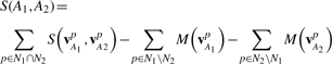Where v_A1^p and v_A2^p are chem-vectors of the same 3D coordinate from A₁ and A₂, respectively and .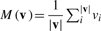

3.6 Sub-cavity clustering and reshaping

We now have a set of sub-cavities which are observed to participate in binding, extracted from a large diverse set of protein–ligand complexes and have specified a similarity function which accounts for sub-cavity shapes and chemical profiles. Using the similarity function, we alternate between clustering and reshaping the sub-cavities. Sub-cavity refinement addresses the fact that the initial sub-cavities naively include all points within a specified distance of a chemical group. Therefore, the sub-cavity may include many points that are neither relevant nor specific to binding. With a goal of accurate functional inference, we employ a reshaping process to increase the functional agreement among those sub-cavities that fall within the same cluster. This procedure is possible with the assumption (confirmed by our experiments) that in their initial state, two sub-cavities with the same label (i.e. associated with the same chemical group) will generally be more similar than two sub-cavities with different labels. Furthermore, we assume that this initial similarity exists because the sub-cavities share a similar substructure. Likewise, sub-cavities can be made more similar by removing the inconsistent structural variations.

The process starts by computing the pairwise similarity of all initial sub-cavities and clustering them using Affinity Propagation (Frey and Dueck, 2007). Following our previous assumption, there will typically be an overrepresented or dominant) label among the sub-cavities of each cluster. Within a cluster, the sub-cavities sharing the dominant label are considered inliers [or true positives (TP)] while the remaining sub-cavities are outliers [or false positives (FP)]. The number of outliers can be reduced by reshaping the inliers toward their maximal common substructure (MCS). We use the Random Sample Consensus algorithm (RANSAC) (Fischler and Bolles, 1981) to identify outliers. Intuitively, the RANSAC algorithm assumes that iterative random sampling of sets of sub-cavities from a cluster will result in an all-inlier subset and that the MCS computed from an all-inlier subset will be both large and consistent. Within the cluster, inconsistent sub-cavities are marked as outliers. The inliers are reshaped by retaining only the structures consistent with the MCS. Once reshaping is complete, we recalculate the new pairwise similarities and cluster again. The process terminates when the clusters no longer change or a maximal number of iterations has elapsed.

4 RESULTS AND DISCUSSION

The current work describes experiments using both simulated and real experimental data. In Section 4.1, we describe an experiment on simulated data in which we identified and clustered a set of generated sub-cavities. The experiments described in Section 4.2 were performed with real experimental data and explore sub-cavity label recovery for a set of functionally similar proteins. These experiments demonstrate the performance of our approach on real sub-cavities. In Section 4.3, we describe the results of an evaluation of a non-redundant set of over 300 protein–small-molecule complexes taken from the PSMDB. We analyze the predictive performance of the resulting clusters and highlight functional inference on the binding sites of HIV-1 Protease and Thrombin. Finally, in Section 4.4 we discuss design decisions, limitations and possible extensions of the presented work.

4.1 Simulated data

We began by evaluating the clustering and reshaping stages of our algorithm (Section 3.6). We tested the ability of our procedure to recover the structure of a sub-cavity template given a set of noisy instances of a template structure. We first randomly generated 20 sub-cavity templates according to the distribution of sub-cavity sizes, number of pseudo-centers and function types found in the sub-cavities extracted from 1754 non-redundant protein–ligand complexes in the PSMDB. For each template, we generated approximately 20 noisy instances or observed sub-cavities. This was done by randomly adding structure grid points adjacent to the sub-cavity surface and altering its pseudo-center locations. The number of random grid points that were added varied from 10% to 40% of the size of the initial sub-cavity. Each experiment was evaluated using the following parameters: (i) homogeneity—the percent of TP within each cluster; (ii) cluster coherence—a measure similar to homogeneity but which penalizes false negatives (FN) (missed relevant sub-cavities); and (iii) net cluster similarity—a measure of the compactness of each cluster. After refinement, 26 clusters (mean cluster size of 15) and 27 clusters (mean cluster size of 13) were found for the 10% and 40% noise experiments, respectively. The additional clusters were formed by splitting a single cluster with consistent labeling into two smaller clusters (data not shown). This is a consequence of Affinity Propagation's automatic selection of the number of clusters—a feature that is considered both an advantage and a disadvantage of the approach.

Homogeneity: we define the homogeneity score of a recovered cluster to be its precision, TP/(TP+FP). This measurement is particularly important when structurally distinct sub-cavities with identical labels are split into multiple clusters. Figure 3A shows the changes in homogeneity gained by each iteration of clustering and reshaping. We found the algorithm to yield a high homogeneity score (0.97–0.99) regardless the amount of noise. We saw a small decrease in the homogeneity of the clusters (<0.02) which can be attributed to the appearance of additional small clusters after reshaping. A single error in a small cluster significantly effects the homogeneity score thereby slightly pulling down the reported averages. This is supported by an increase in the SD of the homogeneity scores.

Fig. 3.

Results on 20 simulated template sub-cavity structures. While the homogeneity scores are fairly consistent during refinement (A) the outlier scores dramatically improve after the first iteration (B). The percentage improvement in net cluster similarity for each noise level is shown in (C). Significant improvement is not observed for the 10% noise experiments as the clusters are already extremely similar. A larger improvement in similarity is observed for experiments run with higher noise levels.

Cluster coherence: the RANSAC algorithm's ability to identify outliers (or FP) during the reshaping step refines the MCS and subsequently improves the cluster quality. The cluster coherence score is calculated as TP/(TP+FP+FN) and is similar to the homogeneity score with an added penalty for FNs. In the context of the simulated sub-cavities, a FN is a sub-cavity that should be included in a given cluster but which is not. The cluster coherence score is relevant primarily for simulated data in which the true number of clusters is known and the algorithm's ability to recover them is tested. Figure 3B illustrates the quality of outlier identification with respect to the reshaping iterations. We see that the reshaping process improves outlier identification regardless of the amount of noise in the data. It is interesting to note that there is almost no improvement in the score after the first reshaping iteration suggesting convergence to a locally optimal solution.

Net cluster similarity: we evaluated the net cluster similarity of the clustering process after each reshaping iteration. Using the cluster exemplar identified by Affinity Propagation, the net similarity is the sum of all similarities between each sub-cavity and its cluster's exemplar plus the sum of all exemplar preferences (Frey and Dueck, 2007). This indicated how well the objective function had been maximized. For example, if we had recovered the optimal structures, the net similarity of every cluster would be maximal. Figure 3C shows the change in net similarity with respect to the reshaping iterations. We see that the net similarity increased with the iterative reshaping process. This implies that the sub-cavities within each cluster became more similar to their exemplar and also to each other.

4.2 Clustering different protein classes

In the second experiment, we evaluated our algorithm on a set of experimentally solved protein–ligand complexes. We assembled a dataset of 80 protein–ligand complexes from the PSMDB database (482 sub-cavities) spanning 6 different enzyme classes. Each protein in the same enzyme class shares the same 3-number prefix of their Enzyme Classification (EC) number (Bairoch, 2000) and catalyzes a similar chemical reaction. We evaluated the recovered clusters by the homogeneity (Section 4.1) of the cluster's most common function type. Our algorithm returned 39 clusters with a mean cluster size of 12 sub-cavities. Figure 4 shows the distribution of cluster scores and demonstrates that most clusters have very high homogeneity.

Fig. 4.

The distribution of homogeneity scores by ligand function type for the six enzyme class experiments. The majority of clusters are highly homogeneous.

4.3 PDB sub-cavity analysis and inference

In order to establish the suitability of our algorithm for inferring protein–ligand interactions, we analyzed large non-redundant datasets of sub-cavities derived from complexes in the PSMDB. In these experiments, we trained our system using one set of protein–ligand complexes and then evaluated the performance of the system using a novel, independent test set. Although the complexes in the training and testing set were different, our prediction was that the complexes would share local or sub-cavity similarity which could then be used to infer sub-cavity binding preferences. Our experiments using two well-characterized protein systems, HIV Protease and Thrombin, confirmed this prediction and highlight the utility of this approach.

4.3.1 Sub-cavity analysis

We extracted 6573 sub-cavities from the PSMDB-25% dataset which contains protein–small-molecule complexes having no >25% protein sequence identity. From this initial set, we created five different random subsets each containing 650 sub-cavities. Each of the five sets was run through our algorithm to obtain clusters and corresponding exemplars. For each cluster we calculated a homogeneity score (similar to Section 4.2) that is the ratio between the highest number of occurrences of any function type and the size of the cluster. We labeled each cluster by the most frequent function type.

For each experiment, we randomly sampled a test set of 300 sub-cavities not included in the training set. Using the similarity function of Section 3.5, we identified the cluster with the most similar exemplar to the query. The homogeneity of the most similar cluster was compared to a set threshold. If the homogeneity score was above a threshold, we made a prediction and compared the label of the cluster to the known label of the sub-cavity. The percent of correctly predicted sub-cavities was reported as the precision of the experiment (Table 1). If a prediction is not made, it is not counted against the precision. Table 1 shows that the best predictions were made by clusters with high homogeneity. This effect became more pronounced if reshaping had been performed. Visual inspection revealed that some of the false predictions occurred when two different chemical groups were located in close proximity. In this situation, the function types' associated cavities were extremely similar and the algorithm had difficulty teasing the two apart. For example, a phenol group shows two proximate function types—a hydrophobic group arising from the benzene ring and a HBD group arising from the associated hydroxyl group. In this case, it is possible for the algorithm to confuse one binding pocket for another. This suggests that a single cluster may support interactions with multiple different chemical groups. A larger training set may provide disambiguation of these cases.

Table 1.

Inference success rate by homogeneity score cutoffs

Reshaping iteration	<0.5	0.5–0.75	0.75–1.00
0	0.61	0.73	0.72
1	0.62	0.73	0.75
2	0.61	0.73	0.84

Clusters having higher homogeneity scores demonstrate better inference precision. The iterative clustering–reshaping process increases the precision for clusters with a higher homogeneity scores. It supports the assumption that the similarity within a cluster comes from the sharing of a common substructure the— reshaping process uncovers this structure and increases prediction accuracy. Clusters with lower homogeneity scores are less likely to share common substructure and benefit less from the reshaping process.

4.3.2 Inference

Toward the goal of automatic sub-cavity-based pharmacophoric inference, we characterize the function type of each sub-cavity within a protein binding site. This was a challenging task for several reasons: any bound ligand may not exploit all possible interaction sites, different bound ligands may satisfy the same interaction site in alternate ways and the presence of a ligand chemical group in a sub-cavity does not necessarily imply that the chemical group is the ideal interaction partner for the associated sub-cavity. Despite these caveats, the set of known binding ligands provided arguably the best source of information for learning sub-cavity binding preferences.

We performed binding inference for two protein systems, HIV-1P and Thrombin. These systems were selected because they are high-profile drug targets for which multiple complex structures had been solved. Starting from the known ligand binding site, we predicted the function type of each sub-cavity and compared these predictions to a set of known binding ligands. We constructed a training set of approximately 650 sub-cavities in a manner similar to Section 4.3.1; however, most importantly, we removed any sub-cavity which originated from either test protein or their homologs.

We applied the algorithm over the training set to produce a set of clustered sub-cavities. Using the function prediction method described in Section 4.3.1 with homogeneity thresholds of 0.65, 0.75 and 0.85 the sub-cavities of the two test proteins were predicted. The predictions were compared to a set of ligands known to bind the specified sub-cavities.

Binding site prediction for HIV-1 Protease: HIV-1 Protease is an aspartic protease responsible for the cleavage of two HIV poly-protein chains into several distinct proteins including the protease itself. The PDB contains structures for a total of nine HIV protease inhibitors which use the structural scaffold illustrated in Figure 5A. For example, the ligand of 1HWR (Ala et al., 1998) contains two phenyl groups (hydrophobic and aromatic) (R3, R7), two 1-butene groups (hydrophobic) (R4, R6), two hydroxyl groups (HBD and HBA) (R1, R2) and one carbonyl group (HBA) (R5). In our experiment, the 1HWR PDB complex was used as the query protein. We extracted seven sub-cavities using three homogeneity score thresholds as shown in Table 2. For five of the seven sub-cavities, the predicted function types strongly agreed with the R-groups observed among the nine ligands. The nearest cluster for two of the sub-cavities had a homogeneity score below the three specified thresholds; therefore, a prediction was not made. None of the HIV-1P proteins or their homologs were used in training which supports the use of our method as a general approach.

Table 2.

Inference results for HIV-1 Protease active site

	R1	R2	R3	R4	R5	R6	R7
Prediction	HBD	HBD	Arom.	Arom.	–	–	Arom.
0.65	8/8	9/9	9/9	8/9	–	–	9/9
0.75	8/8	9/9	9/9	8/9	–	–	9/9
0.85	8/8	–	–	–	–	–	–

Sub-cavity inference results for the binding site of HIV-1 Protease. Using three different homogeneity score thresholds (0.65, 0.75 and 0.85), the predicted sub-cavity labels were compared to a set of nine ligands. R-groups refer to Figure 5A. The predictions made by our algorithm appear in the ‘Prediction’ row (Arom., aromatic). No prediction was made when the cluster's homogeneity score did not pass the set threshold (indicated by a ‘−’). An entry X/Y indicates X correct predictions made for the Y ligands with a corresponding R-group (i.e. not all ligands have a substituted chemical group at each R position).

Binding site prediction for Thrombin: Thrombin is a serine protease involved in the blood coagulation cascade. It catalyzes the conversion of inactive fibrinogen to an active fibrin and participates in activation of other coagulation factors. Consequently, it is a high-profile target for many anticoagulant drugs. The PDB contains the structures of nine thrombin complexes with ligands containing slight variations on a common scaffold. Similar to the HIV-1P example above, the thrombin ligands vary at five R-group positions. For example, the ligand of 3BIU (Gerlach et al., 2007) contains two carbonyl groups (HBA) (R3, R4), one 5-carbon ring group (hydrophobic) (R5), one phenyl group (hydrophobic and aromatic) (R2) and one amidine group (HBD) (R1). The 3BIU PDB complex was used as a query for this experiment. We extracted five sub-cavities corresponding to the five R-groups as shown in Table 3. For three of the five sub-cavities, the predicted function types strongly agree with the R-groups observed among the nine ligands. For each of the remaining two cavities, the nearest cluster had a homogeneity score below the three specified thresholds, thus a prediction was not made. Sub-cavity R1 corresponds to the well-known catalytic triad of Ser, His and Asp often seen in protease enzymes. Interestingly, the cluster containing the R1 sub-cavity had the highest homogeneity value demonstrating the algorithm's ability to learn a highly conserved local motif (i.e. observed across multiple different active sites). As in the previous experiments, no thrombin proteins or their homologs were used in training.

Table 3.

Inference results for Thrombin active site

	R1	R2	R3	R4	R5
Prediction	HBD+HBA	–	HBD+HBA	HBA	–
0.65	6/6	–	9/9	9/9	–
0.75	6/6	–	9/9	–	–
0.85	6/6	–	–	–	–

Sub-cavity inference results for the binding site of Thrombin. Using three different homogeneity score thresholds (0.65, 0.75 and 0.85), the predicted sub-cavity labels were compared to a set of nine ligands. The predictions made by our algorithm appear in the ‘Prediction’ row. No prediction was made when the cluster's homogeneity score did not pass the set threshold (indicated by a ‘−’). An entry X/Y indicates X correct predictions made for the Y ligands with a corresponding R-group (i.e. not all ligands have a substituted chemical group at each R position).

In summary, our algorithm represents a significant step toward fully automated binding site analysis. Using simulated data, we were able to recover known sub-cavity structure in the presence of up to 40% noise. We demonstrated the utility of the iterative clustering and reshaping stages to increase classification accuracy. When run against a set of 80 experimental protein–ligand complexes, our algorithm successfully generated a small number of clusters with high homogeneity. We tested the ability of the algorithm to perform binding inference by training on 650 experimental sub-cavities and then measuring the predictive accuracy on an independent set of 300 different sub-cavities. Our approach achieved a predictive accuracy of 84%. The ability of the algorithm to predict the functional group of a ligand observed to occupy a query sub-cavity should be interpreted in the appropriate context, however. The observation of a chemical group inside a sub-cavity does not necessarily imply a significant interaction. The predicted function type simply reflects the general binding preference of the sub-cavity as observed across a large number of protein–ligand complexes. The chemical groups of any one bound ligand may disagree slightly with the predicted function types providing possible opportunities for lead optimization. In practice, we expect that the predicted types will generally agree with a set of known substrates. This hypothesis was confirmed for both the HIV-1P and Thrombin proteins (Section 4.3.2). Working from this observation, a prediction should only be considered incorrect if the predicted function type is unlikely to interact with the receptor.

4.4 Extensions and limitations

Our method represents a step toward a complete and automatic system for characterizing an active site binding profile. One limitation of the current approach is our reliance on experimentally determined structures of bound protein–ligand complexes. Although these experimental structures provide the highest quality verified structural information on protein–ligand interactions, the number of available complexes is limited. To expand the dataset used in analysis, it may be possible to incorporate the use of experimental structures in the apo form. With respect to inference, it may be possible to predict the location of a protein's binding site (Hendlich et al., 1997; Weisel et al., 2007) and to divide it into hypothesized sub-cavities each of which can be clustered and reshaped using the approach of Section 3.6. A second limitation of our approach is the independence assumption between the binding profiles of neighboring sub-cavities (Pellecchia et al., 2002). We are currently working to incorporate such synergistic effects on binding. With respect to evaluating inference, it is possible we have been too conservative with reporting the performance of our independent training and testing experiments. A TP by our definition requires a known holo structure involving the specified chemical group. In practice, the inferred interaction may indeed be correct; however, there may simply be no experimentally solved structure that can verify it.

The experimental results suggest two final avenues for extension. First, we demonstrated the importance of sculpting sub-cavities toward their maximal common substructure; however, our results suggest that a more sophisticated MCS algorithm (Shatsky et al., 2006) may improve both classification accuracy and structure recovery. Second, although not explicitly discussed in this article, computational challenges may arise when our approach is scaled to include a larger structural dataset (such as the use of apo structures listed above). Accuracy and scalability may be maintained by approximating the similarity matrix of Section 3.5 with an appropriately computed sparse matrix. Fortunately, the affinity propagation clustering algorithm we employed should be consistent with such an approximation.

5 CONCLUSION

We have presented an algorithm that infers binding site patterns by utilizing local similarity among active site sub-cavities. The uniqueness of our approach lies not only in the consideration of sub-cavities, but also in the more complete structural representation of these sub-cavities, their parametrization and the method by which they are compared. We demonstrated the algorithm's ability to leverage previously unused structural information to perform binding inference for proteins that do not share significant structural similarity with known systems. Using HIV-1 Protease and Thrombin as test cases, we have taken the first step toward sub-cavity-based pharmacophore inference. We intend to extend our work toward fully automatic pharmacophore inference and protein function prediction. More specifically, we believe that an automatically generated pharmacophore map could be used for virtual docking, lead optimization and de novo drug design. An example of a lead optimization effort using this approach would be to apply predicted binding preferences to the replacement of chemical groups on a well-studied scaffold. Detailed knowledge of a pharmacophore map may also allow protein function prediction or provide support for human-generated binding hypotheses.

REFERENCES

- Ala PJ, et al. Molecular recognition of cyclic urea HIV-1 protease inhibitors. J. Biol. Chem. 1998;273:12325–12331. doi: 10.1074/jbc.273.20.12325. [DOI] [PubMed] [Google Scholar]
- Bairoch A. The ENZYME database in 2000. Nucleic Acids Res. 2000;28:304–305. doi: 10.1093/nar/28.1.304. [DOI] [PMC free article] [PubMed] [Google Scholar]
- Berman HM, et al. The Protein Data Bank. Nucleic Acids Res. 2000;28:235–242. doi: 10.1093/nar/28.1.235. [DOI] [PMC free article] [PubMed] [Google Scholar]
- Binkowski AT, et al. Inferring functional relationships of proteins from local sequence and spatial surface patterns. J. Mol. Biol. 2003;332:505–526. doi: 10.1016/s0022-2836(03)00882-9. [DOI] [PubMed] [Google Scholar]
- Chen X, et al. Automated pharmacophore identification for large chemical data sets1. J. Chem. Infor. Comput. Sci. 1999;39:887–896. doi: 10.1021/ci990327n. [DOI] [PubMed] [Google Scholar]
- Dror, et al. Predicting molecular interactions in silico: I. an updated guide to pharmacophore identification and its applications to drug design. Front. Med. Chem. 2006;3:551–584. doi: 10.2174/0929867043456287. [DOI] [PubMed] [Google Scholar]
- Fischler MA, Bolles RC. Random sample consensus: a paradigm for model fitting with applications to image analysis and automated cartography. Commun. ACM. 1981;24:381–395. [Google Scholar]
- Frey BJ, Dueck D. Clustering by passing messages between data points. Science. 2007;315:972–976. doi: 10.1126/science.1136800. [DOI] [PubMed] [Google Scholar]
- Gerlach C, et al. Thermodynamic inhibition profile of a cyclopentyl and a cyclohexyl derivative towards thrombin: the same but for different reasons. Angew. Chem. Int. Ed. 2007;46:8511–8514. doi: 10.1002/anie.200701169. [DOI] [PubMed] [Google Scholar]
- Halperin I, et al. Principles of docking: An overview of search algorithms and a guide to scoring functions. Proteins. 2002;47:409–443. doi: 10.1002/prot.10115. [DOI] [PubMed] [Google Scholar]
- Hendlich M, et al. Ligsite: automatic and efficient detection of potential small molecule-binding sites in proteins. J. Mol. Graph. Model. 1997;15 doi: 10.1016/s1093-3263(98)00002-3. [DOI] [PubMed] [Google Scholar]
- James AC, et al. Daylight Theory Manual-Daylight 4.71. Daylight Chemical Information Systems. 2000 Available at www.daylight.com. [Google Scholar]
- Kahraman A, et al. Shape variation in protein binding pockets and their ligands. J. Mol. Biol. 2007;368:283–301. doi: 10.1016/j.jmb.2007.01.086. [DOI] [PubMed] [Google Scholar]
- Kinoshita K, Nakamura H. Identification of protein biochemical functions by similarity search using the molecular surface database eF-site. Protein Sci. 2003;12:1589–1595. doi: 10.1110/ps.0368703. [DOI] [PMC free article] [PubMed] [Google Scholar]
- Kuhn D, et al. From the similarity analysis of protein cavities to the functional classification of protein families using cavbase. J. Mol. Biol. 2006;359:1023–1044. doi: 10.1016/j.jmb.2006.04.024. [DOI] [PMC free article] [PubMed] [Google Scholar]
- Kupas K, et al. Large scale analysis of protein-binding cavities using self-organizing maps and wavelet-based surface patches to describe functional properties, selectivity discrimination, and putative cross-reactivity. Proteins Struct. Funct. Bioinform. 2007;71:1288–1306. doi: 10.1002/prot.21823. [DOI] [PubMed] [Google Scholar]
- Langer T, Hoffmann RD. Pharmacophores and Pharmacophore Searches. 1st. Palo Alto: Wiley-VCH; 2006. [Google Scholar]
- Laskowski RAA, et al. Protein function prediction using local 3D templates. J. Mol. Biol. 2005 doi: 10.1016/j.jmb.2005.05.067. [DOI] [PubMed] [Google Scholar]
- Laskowski RA. SURFNET: a program for visualizing molecular surfaces, cavities, and intermolecular interactions. J. Mol. Graph. 1995;13:323–330. doi: 10.1016/0263-7855(95)00073-9. [DOI] [PubMed] [Google Scholar]
- Leibowitz N, et al. Automated multiple structure alignment and detection of a common substructural motif. Proteins Struct. Funct. Genet. 2001;43:235–245. doi: 10.1002/prot.1034. [DOI] [PubMed] [Google Scholar]
- Levitt DG, Banaszak LJ. Pocket: a computer graphics method for identifying and displaying protein cavities and their surrounding amino acids. J. Mol. Graph. 1992;10:229–234. doi: 10.1016/0263-7855(92)80074-n. [DOI] [PubMed] [Google Scholar]
- McGregor M. A pharmacophore map of small molecule protein kinase inhibitors. J. Chem. Inform. Model. 2007;47:2374–2382. doi: 10.1021/ci700244t. [DOI] [PubMed] [Google Scholar]
- Morris RJ, et al. Real spherical harmonic expansion coefficients as 3D shape descriptors for protein binding pocket and ligand comparisons. Bioinformatics. 2005;21:2347–2355. doi: 10.1093/bioinformatics/bti337. [DOI] [PubMed] [Google Scholar]
- Najmanovich R, et al. Detection of 3D atomic similarities and their use in the discrimination of small molecule protein-binding sites. Bioinformatics. 2008;24:i105–i111. doi: 10.1093/bioinformatics/btn263. [DOI] [PubMed] [Google Scholar]
- Nelder JA, Mead R. A simplex method for function minimization. Comput. J. 1965;7:308–313. [Google Scholar]
- Pellecchia M, et al. NMR in drug discovery. Nat. Rev. Drug Discov. 2002;1:211–219. doi: 10.1038/nrd748. [DOI] [PubMed] [Google Scholar]
- Pennec X, Ayache N. A geometric algorithm to find small but highly similar 3D substructures in proteins. Bioinformatics. 1998;14:516–522. doi: 10.1093/bioinformatics/14.6.516. [DOI] [PubMed] [Google Scholar]
- Powers R, et al. Comparison of protein active site structures for functional annotation of proteins and drug design. Proteins Struct. Funct. Bioinform. 2006;65:124–135. doi: 10.1002/prot.21092. [DOI] [PubMed] [Google Scholar]
- Ramensky V, et al. A novel approach to local similarity of protein binding sites substantially improves computational drug design results. Proteins. 2007;69:349–357. doi: 10.1002/prot.21487. [DOI] [PubMed] [Google Scholar]
- Schmitt S, et al. A new method to detect related function among proteins independent of sequence and fold homology. J. Mol. Biol. 2002;323:387–406. doi: 10.1016/s0022-2836(02)00811-2. [DOI] [PubMed] [Google Scholar]
- Shatsky M, et al. Research in Computational Molecular Biology (RECOMB). Berlin/Heidelberg: Springer; 2005. Recognition of binding patterns common to a set of protein structures; pp. 440–455. [Google Scholar]
- Shatsky M, et al. The multiple common point set problem and its application to molecule binding pattern detection. J. Comput. Biol. 2006;13:407–428. doi: 10.1089/cmb.2006.13.407. PMID: 16597249. [DOI] [PubMed] [Google Scholar]
- Shulman-Peleg A, et al. Prediction of interacting single-stranded rna bases by protein-binding patterns. J. Mol. Biol. 2008;379:299–316. doi: 10.1016/j.jmb.2008.03.043. [DOI] [PMC free article] [PubMed] [Google Scholar]
- Sousa SFF, et al. Protein-ligand docking: current status and future challenges. Proteins. 2006;65:15–26. doi: 10.1002/prot.21082. [DOI] [PubMed] [Google Scholar]
- Stark A, Russell RB. Annotation in three dimensions. PINTS: patterns in non-homologous tertiary structures. Nucleic Acids Res. 2003;31:3341–3344. doi: 10.1093/nar/gkg506. [DOI] [PMC free article] [PubMed] [Google Scholar]
- Wallace AC, et al. TESS: a geometric hashing algorithm for deriving 3D coordinate templates for searching structural databases. Application to enzyme active sites. Protein Sci. 1997;6:2308–2323. doi: 10.1002/pro.5560061104. [DOI] [PMC free article] [PubMed] [Google Scholar]
- Wallach I, Lilien R. The protein-small-molecule database, a non-redundant structural resource for the analysis of protein-ligand binding. Bioinformatics. 2009;25:615–620. doi: 10.1093/bioinformatics/btp035. [DOI] [PubMed] [Google Scholar]
- Weisel M, et al. Pocketpicker: analysis of ligand binding-sites with shape descriptors. Chem. Cent. J. 2007;1:7. doi: 10.1186/1752-153X-1-7. [DOI] [PMC free article] [PubMed] [Google Scholar]