A partition function algorithm for interacting nucleic acid strands

Abstract

Recent interests, such as RNA interference and antisense RNA regulation, strongly motivate the problem of predicting whether two nucleic acid strands interact.

Motivation: Regulatory non-coding RNAs (ncRNAs) such as microRNAs play an important role in gene regulation. Studies on both prokaryotic and eukaryotic cells show that such ncRNAs usually bind to their target mRNA to regulate the translation of corresponding genes. The specificity of these interactions depends on the stability of intermolecular and intramolecular base pairing. While methods like deep sequencing allow to discover an ever increasing set of ncRNAs, there are no high-throughput methods available to detect their associated targets. Hence, there is an increasing need for precise computational target prediction. In order to predict base-pairing probability of any two bases in interacting nucleic acids, it is necessary to compute the interaction partition function over the whole ensemble. The partition function is a scalar value from which various thermodynamic quantities can be derived. For example, the equilibrium concentration of each complex nucleic acid species and also the melting temperature of interacting nucleic acids can be calculated based on the partition function of the complex.

Results: We present a model for analyzing the thermodynamics of two interacting nucleic acid strands considering the most general type of interactions studied in the literature. We also present a corresponding dynamic programming algorithm that computes the partition function over (almost) all physically possible joint secondary structures formed by two interacting nucleic acids in O(n⁶) time. We verify the predictive power of our algorithm by computing (i) the melting temperature for interacting RNA pairs studied in the literature and (ii) the equilibrium concentration for several variants of the OxyS–fhlA complex. In both experiments, our algorithm shows high accuracy and outperforms competitors.

Availability: Software and web server is available at http://compbio.cs.sfu.ca/taverna/pirna/

Contact: cenk@cs.sfu.ca; backofen@informatik.uni-freiburg.de

Supplementary information: Supplementary data are avaliable at Bioinformatics online.

1 INTRODUCTION

Starting with the discovery of microRNAs (miRNAs) and the advent of genome-wide transcriptomics, it has become clear that RNA plays a large variety of important roles in living organisms that extend far beyond being a mere intermediate in protein biosynthesis (Storz, 2002). Several of these non-coding RNAs (ncRNAs) regulate gene expression post-transcriptionally through base pairing (and establishing a joint structure) with a target mRNA, as per the eukaryotic miRNAs and small interfering RNAs (siRNAs) (Bartel, 2004; Hannon, 2002; Zamore and Haley, 2005), antisense RNAs (Brantl, 2002; Wagner and Flardh, 2002) or bacterial small regulatory RNAs (sRNAs) (Gottesman, 2005). In addition to such endogenous regulatory ncRNAs, antisense oligonucleotides have been used as exogenous inhibitors of gene expression; antisense technology is now commonly used as a research tool as well as for therapeutic purposes. Furthermore, synthetic nucleic acids systems have been engineered to self-assemble into complex structures performing various dynamic mechanical motions (Seeman, 2005; Seeman and Lukeman, 2005; Simmel and Dittmer, 2005; Venkataraman et al., 2007; Yin et al., 2008).

Despite all the above advances, computational methods for predicting ncRNA–target mRNA interactions suffer from a low specificity (see below for an overview); this is possibly due to two technical reasons. First, several of these methods consider restricted versions of the problem (e.g. simplified energy functions or restricted types of interactions)—this is mostly for computational reasons. Second, a quantitative analysis of binding thermodynamics between oligonucleotides and target RNAs is often lacking. To determine the binding effectiveness, an accurate analysis of the thermodynamics of two interacting nucleic acid strands is necessary.

In this article, we aim to compute how likely two RNA or DNA strands are to interact, and to predict base-pairing probability of any two bases—which we then use to quantitatively measure the strength, probability and stability of the joint structure established by the interacting strands (Mathews, 2004). To correctly calculate those probabilities, it is necessary to compute the partition function over the whole ensemble of possible individual and joint secondary structures. The partition function is a scalar value from which various thermodynamic quantities can be derived (Landau and Lifshitz, 1969). For instance, one can compute the equilibrium concentration of each complex nucleic acid species from their partition functions. Also, the partition function can be used to predict the melting temperature of interacting nucleic acids.

Although algorithms for predicting the most likely (the lowest total free energy) joint structure that can be formed by two interacting RNA strands are available [see, for example, Alkan et al. (2006)], previous little work has been done for computing the partition function of interacting RNA strands. It is important to note that designing an algorithm to compute the partition function is more challenging than that to predict the minimum free energy secondary structure: a partition function algorithm should guarantee that every joint structure is considered exactly once.

In this article, we present an O(n⁶) time algorithm to compute the partition function over the type of interactions that Alkan et al. (2006) considered.¹ We extend the standard energy model for a single RNA model to an energy model for the joint secondary structure of interacting strands by considering new types of (joint) structural components. We verify our algorithm (and the associated software we developed) by computing the melting temperature for RNA pairs available (Diamond et al., 2001; Mathews and Turner, 2002; Xia et al., 1998) and the equilibrium concentration for OxyS–fhlA complexes for wild-type fhlA and four other mutants reported in the literature (Argaman and Altuvia, 2000). In both experiments, our algorithm shows high accuracy and outperforms existing alternatives.

1.1 Related work

During the last few decades, several computational methods emerged to study the secondary structure thermodynamics of a single nucleic acid strand. Nearest neighbor thermodynamic model has become the standard energy model for a nucleic acid secondary structure (Mathews et al., 1999). The standard energy model is based on the assumption that stacking base pairs and loop entropies contribute additively to the free energy of a nucleic acid secondary structure. More recently, the standard energy model has been extended for pseudoknots (Cao and Chen, 2006; Dirks and Pierce, 2003). Based on additivity of the energy, efficient dynamic programming algorithms for predicting the minimum free energy secondary structure (Nussinov et al., 1978; Rivas and Eddy, 1999; Waterman and Smith, 1978; Zuker and Stiegler, 1981) and computing the partition function of a single strand (Dirks and Pierce, 2003; McCaskill, 1990) have been developed.

Some previous attempts to analyze the thermodynamics of multiple interacting strands concatenate input sequences in some order and consider them as a single strand. For example, pairfold (Andronescu et al., 2005) and RNAcofold from Vienna package (Bernhart et al., 2006) concatenate the two input sequences into a single strand and predict its minimum free-energy structure. Dirks et al. (2007) present a method, as a part of NUPack, that concatenates the input sequences in some order, carefully considering symmetry and sequence multiplicities, and computes the partition function for the whole ensemble of complex species. However, concatenating the sequences is not accurate at all as even if pseudoknots are considered, some useful interactions are excluded while many physically impossible interactions are included (e.g. physically impossible crossing interactions).

Alternatively, several methods avoid internal base-pairing in either strand, and compute the minimum free energy secondary structure for their hybridization under this constraint [RNAhybrid (Rehmsmeier et al., 2004), UNAFold (Dimitrov and Zuker, 2004; Markham and Zuker, 2008), and RNAduplex from Vienna package (Bernhart et al., 2006)]. These approaches naturally work only for simple cases involving typically very short strands.

A third set of methods predict the secondary structure of each individual RNA independently, and predict the (most likely) hybridization between the unpaired regions of the two molecules. More sophisticated alternatives view interaction as a multi-step process (Busch et al., 2008; Mückstein et al., 2006; Walton et al., 2002): (i) unfolding of the two molecules to expose bases needed for hybridization, (ii) the hybridization at the binding site and (iii) restructuring of the complex to a new minimum free-energy conformation.

In addition to the above approaches, a number of studies aimed to compute the minimum total energy joint structure between two interacting strands under energy models with growing complexity. For instance, Pervouchine devised a dynamic programming algorithm to maximize the number of base pairs among interacting strands (Pervouchine, 2004). A follow-up work by Kato et al. (2009) proposed a grammar-based approach to RNA–RNA interaction prediction. More generally, Alkan et al. (2006) studied the joint secondary structure prediction problem under three different models: (i) base pair counting, (ii) stacked pair energy model and (iii) loop energy model. Alkan et al. (2006) proved that the general RNA–RNA interaction prediction under all three energy models is an NP-hard problem. Therefore, they suggested some natural constraints on the topology of possible joint secondary structures that are satisfied by all examples of complex RNA–RNA interactions in the literature. The resulting algorithms compute the minimum free energy secondary structure among all possible joint secondary structures that do not contain (internal) pseudoknots, crossing interactions (i.e. external pseudoknots) and zigzags (see Section 2.1 for the exact definition).

2 METHODS

2.1 Preliminaries

Throughout this article, we denote the two nucleic acid strands by R and S. Strand R is indexed from 1 to L_R, and S is indexed from 1 to L_S both in 5^′ to 3^′ direction. Note that the two strands interact in opposite directions, e.g. R in 5^′ → 3^′ with S in 3^′ ← 5^′ direction. Each nucleotide is paired with at most one nucleotide in the same or the other strand. We refer to the i-th nucleotide in R and S by i_R and i_S, respectively. The subsequence from the i-th nucleotide to the j-th nucleotide in a strand is denoted by [i, j].

An intramolecular base pair between the nucleotides i and j in a strand is called an arc and denoted by a bullet i•j. An intermolecular base pair between the nucleotides i_R and i_S is called a bond and denoted by a circle i_R○i_S. An arc i_R•j_R covers a bond l_R○k_S if i_R<l_R<j_R. We call i_R•j_R an interaction arc if there is a bond l_R○k_S covered by i_R•j_R. A kissing arc is an interaction arc that directly covers a bond. More precisely, we call i_R•j_R a kissing arc if it covers a bond l_R○k_S such that if i_R′•j_R′ covers the same bond l_R○k_S, then i_R′≤i_R and j_R≤j_R′. A subsequence [i_R,j_R] contains a direct bond, l_R○k_S, if i_R≤l_R≤j_R and no arc within [i_R,j_R] covers l_R○k_S. Assuming i_R<j_R, two bonds i_R○i_S and j_R○j_S are called crossing bonds if i_S<j_S. An interaction arc i_R•j_R in a strand subsumes a subsequence [i_S,j_S] in the other strand if for all bonds l_R○k_S, if i_S≤k_S≤j_S then i_R<l_R<j_R. Two interaction arcs are equivalent if they subsume one another. Two interaction arcs i_R•j_R and i_S•j_S are part of a zigzag, if neither i_R•j_R subsumes [i_S,j_S] nor i_S•j_S subsumes [i_R,j_R].

In this article, we assume there are no pseudoknots in individual secondary structures of R and S, and also there are no crossing bonds and zigzags between R and S.

2.2 Interaction energy model

An unpseudoknotted secondary structure s of a single nucleic acid, in the standard energy model (Mathews et al., 1999), is decomposed into loops, and a free energy is associated with every loop in s. The total free energy G_s is the sum of loop free energies. The standard model consists of the following loop types: (i) hairpin, (ii) interior, which can be stack, bulge or internal loop and (iii) multiloop whose energies are denoted by G^hairpin, G^interior and G^multi, respectively.

In an interaction, secondary structure of two strands under our assumptions (remember we do not allow pseudoknots, crossing bonds and zigzags in this work), new kinds of components can appear. We extend the standard energy model by defining those new kinds of interaction components. Similar to the standard case, an interaction secondary structure s can be decomposed into intramolecular loops and the new interaction components such that the total free energy G_s is sum of the free energies of loops and interaction components. Figure 1 shows the decomposition of OxyS–fhlA pair secondary structure into the interaction components (Argaman and Altuvia, 2000). These components and their free energy contributions are

• Hybrid: G^hybrid_{{kⁱR○kⁱS}} is the free energy of a joint secondary structure consisting of a series of bonds, kⁱ_R○kⁱ_S, i=1,…, m, with no intramolecular base pairing or branching. We call such a component hybrid. We define the energy associated with a hybrid component by

  (1)

  in which β₁ is the penalty for the formation of the hybrid, and σ ≤ 1 is the ratio of the free energy of intermolecular to that of intramolecular interior loops [as suggested by Alkan et al. (2006)] (Fig. 2). Note that with β₁=0, σ=1, G^hybrid is identical to the energy proposed by RNAhybrid, first introduced by Rehmsmeier et al. (2004), which considers only one hybrid component for mRNA/target duplexes and does not allow any intramolecular structure.
• Kissing: G^kissing_U^k,B^k is the energy of an intramolecular loop (hairpin, interior or multiloop) that makes interaction with the other strand. Such component is called a kissing loop. The energy associated with a kissing loop is given by

  (2)

  in which B^k is the number of loops and U^k the number of unpaired bases in the kissing loop (Fig. 3). Note that in our model we use different β₁ and σ values for a hybrid component covered by a kissing loop.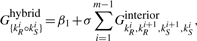

• Inter-hybrid: G^inter-hybrid is the energy of an intermolecular loop bounded by two bonds belonging to two consecutive hybrid components. Bases in either sequence facing this kind of loop might be the end points of only arcs and not bonds. We call such a component inter-hybrid loop. In this work, the energy contribution of an inter-hybrid loop is assumed to be 0.

Fig. 1.

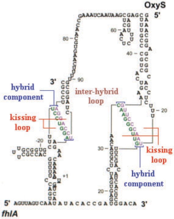
Interaction components of OxyS–fhlA pair presented in Argaman and Altuvia (2000).

Fig. 2.

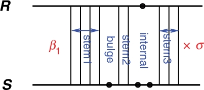
A hybrid component between the two strands whose free energy is G^hybrid=β₁+σ(G^stem₁+G^bulge+G^stem₂+G^internal+G^stem₃).

Fig. 3.

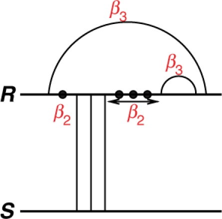
A kissing loop in R that interacts with the other strand S. In this case, the free energy of the kissing loop is G^kissing=4β₂+2β₃.

2.3 Interaction partition function

The partition function is a weighted sum over the set of all possible secondary structures S

(3)

where R is the universal gas constant and T is the temperature.

Efficient algorithms for computing the partition function for a single strand have been given. McCaskill (1990), gave the first partition function algorithm for a single unpseudoknotted nucleic acid strand and Dirks and Pierce (2003) gave a partition function algorithm for a single strand allowing pseudoknots. However, computing the partition function for multiple interacting strands has not been properly addressed. In previous attempts, multiple strands are concatenated in some order and partition function for the resulting single strand is computed (Bernhart et al., 2006; Dimitrov and Zuker, 2004; Dirks et al., 2007). That approach is not accurate as even if pseudoknots are considered, some useful interactions are excluded while many physically impossible interactions are included (e.g. physically impossible crossing interactions). On the other hand, considering all possible secondary structures makes the problem NP-hard (Alkan et al., 2006). Therefore, we only consider those secondary structures that do not contain pseudoknots, crossing bonds and zigzags.

Interaction partition function (IPF) problem

Given a pair of nucleic acid strands R and S, and a temperature T, compute the partition function, QI(T), over SI the set of all possible single or duplex secondary structures that do not contain pseudoknots, crossing bonds and zigzags.

Input: nucleic acid strands R and S.

Output:

We give a recursive algorithm, called Partition function for InteRacting Nucleic Acids (piRNA), for the IPF problem. In all of our recursions, the considered cases are disjoint. This fact shows that every possible secondary structure is reached by exactly one trajectory in the recursion process. Our algorithm guarantees to consider all possible secondary structures exactly once. Since our algorithm covers so many cases, we do not include all the details here. A comprehensive description of our algorithm is available in our Supplementary Material.

We present our algorithm using recursion diagrams (Dirks and Pierce, 2003; Rivas and Eddy, 1999). Our algorithm computes two types of recursive quantities: (i) the partition function of a subsequence [i, j] in one strand, and (ii) the joint partition function of subsequences [i_R, j_R] and [i_S,j_S]. A region is the domain over which a partition function is computed. Terminal bases are the boundaries of a region. For the first type, region is [i, j] with i and j terminal bases. For the second type, region is [i_R,j_R] × [i_S,j_S] with i_R, j_R, i_S and j_S terminal bases. The length pair of region [i_R,j_R] × [i_S,j_S] is (l_R=j_R − i_R + 1, l_S=j_S − i_S + 1). Our algorithm starts with (l_R = 1, l_S = 1) and considers all length pairs incrementally up to (l_R = L_R, l_S = L_S). For a fixed length pair (l_R, l_S), recursive quantities for all the regions [i_R, i_R + l_R − 1] × [i_S, i_S+l_S − 1] are computed.

For computing the partition function of a subsequence in one strand we use McCaskill's (1990) algorithm. McCaskill's algorithm is shown in Figure 4, in which Q_i,j is the partition function for the subsequence [i, j]. Throughout this article, a horizontal line indicates the phosphate backbone, a solid curved line indicates an arc and a dashed curved line encloses a region and denotes its two terminal bases that may be paired or unpaired. Letter(s) within a region specify a recursive quantity. White regions are recursed over and blue regions indicate those portions of the secondary structure that are fixed at the current recursion level and contribute their energy to the partition function as defined by the energy model. Green and red regions have the same recursion cases as the corresponding white regions, except that for the green regions multiloop energy and for red regions kissing loop energy is applied, i.e. the corresponding penalties for each unpaired base and base pair should be applied.

Fig. 4.

McCaskill's algorithm: recursion for Q_i,j, the partition function for the subsequence [i, j]. Above, Q^b_i,j is the partition function for the subsequence [i, j] assuming i and j are base paired, and Q^bz_i,j is the partition function for the subsequence [i, j] assuming there is at least one arc in the region.

In Figure 4, the first case of Q_i,j corresponds to an empty structure (that constitutes no base pairs) whose free energy is assumed to be 0, thus its contribution to the partition function is e^{−Gempty_{i, j}/RT}=1. In the other case, there exists at least one arc and the leftmost one is k₁•k₂. It contributes Q^b_k1,k2Q_k2+1,j to the partition function, therefore,

(4)

The second line shows the cases of Q^b_i,j which is the partition function for the subsequence [i, j] assuming i and j are base paired. The arc i • j can close different substructures: hairpin, interior or multiloop. The energy contribution of each substructure is calculated based on the standard thermodynamics energy model. The third line shows cases of Q^bz_i,j which is the partition function for the subsequence [i, j] assuming the region constitutes at least one arc. A region tagged by bz and colored by green is contained in a multiloop and the penalty of multiloop should be applied to it. Explicit equations for Q^b_i,j and Q^bz_i,j are given in the Supplementary Material.

In the following, we present all cases of Q^I_iR,jR,iS,jS which is the interaction partition function for the region [i_R,j_R] × [i_S,j_S]. A solid vertical line indicates a bond, a dashed vertical line denotes two terminal bases of a region which may be base paired or unpaired and a dotted vertical line denotes two terminal bases of a region which are assumed to be unpaired. For the interaction partition functions, gray regions indicate a reference to the partition functions for the single sequences. Figure 5 shows the cases of Q^I: (i) there is no bond between the two subsequences, (ii) the leftmost bond is a direct bond in both subsequences and (iii) the leftmost bond is covered by an arc in at least one subsequence. Therefore,

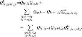(5)

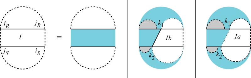
in which Q^Ib_k1,jR,iS,k2 is the interaction partition function for the region [k₁, j_R] × [i_S, k₂] assuming k₁ ○ k₂ is a bond, and Q^Ia_k1,jR,iS,k2 is the interaction partition function for the region [k₁, j_R] × [i_S, k₂] assuming that the leftmost bond in the region is covered by an arc in at least one subsequence. Figures 6 and 8 show the recursion for Q^Ib and Q^Ia where b stands for bond and a stands for arc.

Fig. 5.

Cases of the interaction partition function Q^I_iR,jR,iS,jS. The first case constitutes no bonds. In the second case, the leftmost bond is a direct bond on both subsequences. In the third case, the leftmost bond is covered by an interaction arc in at least one subsequence.

Fig. 6.

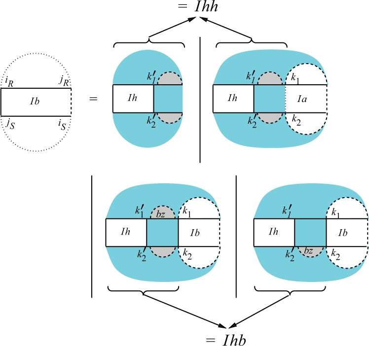
Recursion for Q^Ib_iR,jR,iS,jS assuming i_R○j_S is a bond. We show a version of the recursion that contains two split points in each sequence for simplicity reasons. However, this would increase the complexity and can easily be resolved by introducing two additional matrices Q^Ihh and Q^Ihb for the region [i_R,k₁] × [k₂, j_S] as indicated by the arrows (see Supplementary Material for a full definition).

Fig. 8.

Cases of Q^Ia_iR,jR,iS,jS, for which we assume at least one of i_R and j_S is the end point of an interaction arc.

Figure 6 shows the recursion for Q^Ib_iR,jR,iS,jS, the interaction partition function for the region [i_R, j_R] × [i_S, j_S] assuming i_R○j_S is a bond. Since we have a β₁ penalty for each hybrid component, the recursion for Q^Ib has to determine whether the region contains one or several hybrid components. In all cases, Q^Ih contains the full hybrid component containing the bond i_R○j_S (see Fig. 7 for Q^Ih recursion). The first possibility reflects the case where we have only one hybrid component. In the other cases, we have always at least two hybrid components. The subsequent intermolecular bond starts a new hybrid component iff (i) it is not direct in at least one subsequence, i.e. it is covered by an arc in the associated regions (Case 2 of the Q^Ib recursion), or (ii) there is at least one arc between the two successive intermolecular bonds (Cases 3 and 4 of the Q^Ib recursion). Using the additional matrices Q^Ihh and Q^Ihb, we get

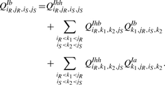(6)

Fig. 7.

Cases of Q^Ih_iR,jR,iS,jS the interaction partition function for a single hybrid component.

Figure 7 shows the cases of Q^Ih: (i) there is no bond other than i_R○j_S and i_S○j_R in the region, and (ii) there exist more bonds between i_R○j_S and i_S○j_R, the leftmost of which is k₁○k₂.

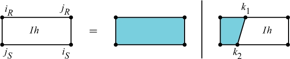
Figure 8 shows the cases of Q^Ia_iR,jR,iS,jS for which at least one of i_R and j_S is the end point of an interaction arc: (i) i_R•k₁ subsumes [k₂, j_S] and k₂ is not base paired with j_S, (ii) k₂•j_S subsumes [i_R, k₁] and i_R is not base paired with k₁ and (iii) i_R•k₁ and k₂•j_S are equivalent. If just one of i_R and j_S is the end point of an interaction arc while the other one is the end point of a bond, then the interaction arc subsumes the other subsequence. If both i_R and j_S are end points of interaction arcs, then one of the arcs subsumes the other one or they are equivalent. Therefore,

(7)

in which Q^Is_iR,k1,k2,jS is the interaction partition function of [i_R, k₁] × [k₂, j_S] assuming i_R•k₁ is an interaction arc that subsumes [k₂, j_S], Q^Is′_iR,k1,k2,jS is the symmetric counterpart of Q^Is and Q^Ie_iR,k1,k2,jS is the interaction partition function of [i_R, k₁] × [k₂, j_S] assuming i_R•k₁ and k₂•j_S are equivalent interaction arcs.

For Q^Ie, it does not make any difference which one of the covering arcs, i_R•j_R and i_S•j_S, is extracted first. We first extract the covering arc from S (Fig. 9). Extracting the covering arc, the remaining subsequence of S contains either at least one direct bond, in which case kissing loop penalty should be applied, or multiple interaction arcs, in which case multiloop penalty should be applied. Hence, Figure 9 is appropriately colored by green and red to remind the type of penalty.

Fig. 9.

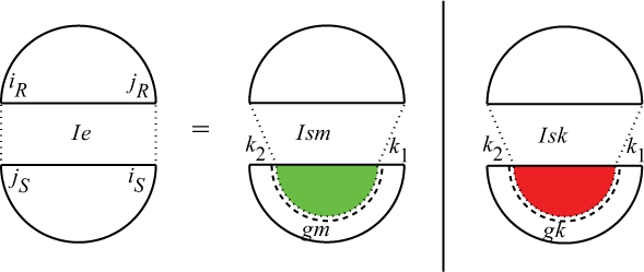
Cases of Q^Ie_iR,jR,iS,jS, for which i_R•j_R and i_S•j_S are equivalent interaction arcs.

Note that Q^gk_i,d,e,j and Q^gm_i,d,e,j are the partition functions for [i, j] excluding the gap [d, e] assuming i and j are base paired. For Q^gk, the gap is assumed to contain a direct bond, and for Q^gm the gap is assumed to contain multiple interaction arcs (Fig. 10). The only difference between Q^gk and Q^gm is in the penalty type. For both Q^gk and Q^gm, there are two cases: (i) there is no more spanning interaction arc in the region, and (ii) there is at least another innermost spanning interaction arc k₁•k₂. In both groups, there could be some additional intramolecular structure in the region. The quantity Q^g_i,k1,k2,j is the partition function for the subsequence [i, j] excluding the gap [k₁, k₂] assuming i•j and k₁•k₂. The gap partition function Q^g is similar to Q^g in Dirks–Pierce's (2003) algorithm. See our Supplementary Material for the details of Q^gk, Q^gm and Q^g.

Fig. 10.

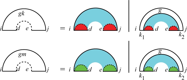
Recursion for Q^gk_i,d,e,j and Q^gm_i,d,e,j, the partition functions for [i, j] excluding the gap [d, e], assuming i and j are base paired. The gap in Q^gk is assumed to contain a direct bond hence the red color, and the gap in Q^gm is assumed to contain multiple interaction arcs hence the green color. In both cases, i<k₁≤d and e≤k₂<j.

The union of the cases of Q^Isk and Q^Ism comprises the cases of Q^Is. Similar to the cases of Q^Ie, we extract the covering arc from Q^Isk and Q^Ism to obtain Q^Imm, Q^Imk, Q^Ikm and Q^Ikk, where k stands for kissing (or equivalently containing a direct bond) and m for multiple interaction arcs. Note that all four terminal bases of the region of these four quantities are paired, i.e. each terminal base is either the end point of a bond or of an interaction arc. These four quantities have complicated cases. Due to lack of space, we explain them in our Supplementary Material.

3 EXPERIMENTS

Here, we report our implementation of the algorithm and two types of experiments we performed to test the predictive power of our algorithm:

1. Predicting the melting temperature of RNA duplexes is an important application of the partition function for interacting nucleic acid pairs (Dimitrov and Zuker, 2004); our first experiment tests how accurately our algorithm predicts the melting temperature of RNA pairs collected from several sources in the literature with respect to the accuracy of available alternatives, RNAcofold from Vienna package v1.7.2 (Bernhart et al., 2006) and UNAFold v3.6 which is a new version of former mfold (Markham and Zuker, 2008). We remind the reader that RNAcofold concatenates the two RNA strands and computes the partition function for the resulting single strand. Therefore, it does not consider many cases that our algorithm considers. UNAFold v3.6, on the other hand, simplifies the problem by forbidding intramolecular base pairing. It computes the partition function of the two strands over just hybridization structures. As can be expected, our algorithm consistently outperforms the alternatives in all three datasets.

2. A novel experiment (which, to our knowledge has not been performed successfully by any other program to date) uses our algorithm to predict the equilibrium concentration of an RNA–RNA complex, in particular the OxyS–fhlA interaction (Argaman and Altuvia, 2000).² We successfully predicted the equilibrium concentrations for OxyS with wild-type fhlA and four other fhlA mutants.

Note that the parameters used by our program in the above experiments have been manually optimized as computational learning methods for fine tuning the parameters require prohibitive computational resources. It may be possible to improve the accuracy of our program through a better selection of parameters.

3.1 Implementation

We remind the reader that the time and space complexity of our algorithm are O(n⁶) and O(n⁴), respectively; here n=max(L_R, L_S) is the maximum length of the two input strands. We implemented our algorithm in C++, and used the energy functions and energy parameters of UNAFold v3.6 for a single strand (Markham and Zuker, 2008). The parameters used by our program for our own interaction energy model are given in the next section. As per Section 2.2, we use a different β₁ penalty and σ for a hybrid component that is covered by a kissing loop. The parameters for a hybrid component that is not covered by a kissing loop is denoted by β′₁ and σ′. We add an Adenine-Uracil base pair (AU) penalty to the energy of a hybrid component per each terminal AU base pair; this penalty is motivated by Xia et al. (1998). Similar to RNAhybrid, the interior loops in a hybrid component are restricted to a constant maximum length, in either sequence, which is set to 15 in this work.

Since our algorithm considers many more possible secondary structures in comparison to alternative methods, our program has a higher running time. Fortunately, our algorithm can be easily parallelized as the dynamic programming tables computed by our program on subsequence pairs depend only on their (proper) subregions. We parallelized our program using OpenMP 3.0. Our experiments were performed on a large-scale shared memory parallel platform with 64 PPC 1.9 GHz processors with 256 GB RAM. We ran our program for strands of length between 5 nt to 120 nt. The running time of our program for short strands (∼20 nt) was < 1 m—for longer strands (∼ 120 nt) it was ∼ 10 h.

3.2 Datasets

The first dataset that we used for predicting melting temperature contains all nine different RNA pairs reported in Table 3 of Xia et al. (1998). It contains almost complementary 5- to 7- nt RNA pairs that were designed to optimize the thermodynamic parameters for terminal base pairs. Their melting temperatures vary from 29.8^○C to 53.7^○C.

Table 3.

Experimental and predicted melting temperatures for the set of RNA pairs reported in Mathews and Turner (2002)

Pairs	Experiment		piRNA		RNAcofold		UNAFold
	Tl	Tc
G-GC-G/C-C	45.4	46	56.81		37		21.4
G-GC-G/CaC	51.8	52.2	56.84		37		27.15
G-GC-G/Ca2C	55.9	56	56.86		37		27.12
G-GC-G/Ca3C	58.4	57.3	56.85		37		25.73
G-GC-G/CauaC	57.3	56.9	56.84		37		24.35
G-GC-G/Ca4C	56.7	57.1	56.85		37		25.06
GaGC-G/C-C	51.2	49.3	56.94		37.1		21.25
GaGC-G/CaC	55.2	54.7	56.96		41		21.44
GaGC-G/Ca2C	56.1	55.6	56.98		41		21.46
GaGC-G/Ca3C	56.1	54.9	56.97		41		21.44
GaGC-G/CauaC	54.8	54.3	56.98		37.06		21.47
GaGC-G/Ca4C	55.3	54.8	56.98		37		21.39
Ga2GC-G/C-C	55.1	52.9	57		50.17		36.04
Ga2GC-G/CaC	57	56.4	57.03		48.01		36.8
Ga2GC-G/Ca2C	55.6	55.4	57.05		41.84		36.91
Ga2GC-G/Ca3C	55	54.7	57.03		41.84		36.19
Ga2GC-G/CauaC	55.3	54.5	57.3		52.17		36.74
Ga2GC-G/Ca4C	54.1	53.9	57.05		48.01		34.22
Ga2GCaG/C-C	56.6	56.6	57.18		47.01		36.01
Ga2GCaG/CaC	58.7	58.9	57.18		44.1		36.81
Ga2GCaG/Ca2C	58	58.8	57.2		44.1		36.13
Ga2GCaG/Ca3C	56.5	57.5	57.15		44.1		36.96
Ga2GCaG/CauaC	57.2	56.9	57.48		43		35.92
Ga2GCaG/Ca4C	57.9	57.9	57.17		44.1		34.66
Ga2GCa2G/C-C	56	56.9	57.19		37.17		36.14
Ga2GCa2G/CaC	58.7	59.1	57.2		44.1		36.94
Ga2GCa2G/Ca2C	59.7	59.6	57.19		44.1		36.22
Ga2GCa2G/Ca3C	58.6	58.7	57.16		44.1		35.89
Ga2GCa2G/CauaC	57	57.3	57.74		37		35.03
Ga2GCa2G/Ca4C	57.5	58.1	57.18		44.1		34.93
G-UA-G/C-C	50.4	50.8	56.82		46.26		21.53
G-UA-G/CaC	54.3	55.8	57.88		61.42		34.47
G-UA-G/Ca2C	56.6	57.8	57.89		61.42		41.68
G-UA-G/Ca3C	57.6	58.5	57.88		61.42		40.84
G-UA-G/CauaC	57.9	58.7	57.87		61.41		40.96
G-UA-G/Ca4C	58.6	58.5	57.88		61.43		40.64
GaUA-G/C-C	51.6	51.8	56.96		49.18		21.42
GaUA-G/CaC	55.6	55.7	57.01		37.07		30.98
GaUA-G/Ca2C	56.7	57.4	57.04		50.31		31.46
GaUA-G/Ca3C	56.8	56.9	57		44.17		29.91
GaUA-G/CauaC	57	57.1	56.99		37.07		29.98
GaUA-G/Ca4C	56.8	56.8	57.01		50.31		29.29
G-CG-GC-G/C-C	64.8	65.2	57.24		37		21.38
G-CG-GC-G/CaC	58.8	60.4	57.22		37		21.44
G-CG-GC-G/Ca2C	55.6	56.4	57.35		37		21.38
G-CG-GC-G/Ca3C	55.4	55.3	57.32		37		21.56
G-CG-GC-G/Ca4C	53.9	53	57.19		37		21.38
GaCG-GC-G/C-C	57.3	58.7	57.2		37		21.71
GaCG-GC-G/CaC	59.7	61.2	57.21		37		21.76
GaCG-GC-G/Ca2C	55.4	57.2	57.19		37		21.45
GaCG-GC-G/Ca3C	55.2	56.5	57.11		37		21.42
GaCG-GC-G/CauaC	55.2	55.8	57.09		37		21.38
GaCG-GC-G/Ca4C	55	55.3	57.14		37		21.47
GaCG-GCaG/C-C	58.1	58.8	56.9		37		21.54
GaCG-GCaG/CaC	59.3	59.7	56.99		37		21.76
GaCG-GCaG/Ca2C	57.5	59.4	56.89		37		63.08
GaCG-GCaG/Ca3C	57.9	58.2	56.95		37		21.44
GaCG-GCaG/CauaC	58.9	58.3	56.93		37		21.53
GaCG-GCaG/Ca4C	57.3	58.1	56.84		37		21.46
Ga2CGa2GCa2G/C-C	54.4	55.5	57.12		47.17		67.28
Ga2CGa2GCa2G/CaC	55	56.6	57.04		44.01		67.23
Ga2CGa2GCa2G/Ca2C	55.3	57.2	57.12		51.31		66.09
		Tl	Tl	Tc	Tl	Tc	Tl	Tc
Avg. difference		0.7	1.87	1.95	14.27	14.41	26.5	26.56
Spearman rank corr.		0.92	0.25	0.35	−0.04	−0.04	0.2	0.28

Each pair is referred to by an identifier. Please refer to our Supplementary Material or Mathews and Turner (2002) to see the exact sequences of each pair. All values, except Spearman's rank correlation, are in degree centigrade. Bold entries are the most accurate predictions. In other words, they have the least difference from experimental measurements.

The second dataset that we used for computing melting temperature contains all 12 different RNA pairs reported in Table 1 of Diamond et al. (2001). These RNA pairs are designed to optimize the thermodynamic parameters for three-way multi loops. In each pair of this dataset, the first RNA has ∼20 nt and the second one has ∼10 nt. The experimental melting temperatures were determined from heat absorbance measurements by two different methods that are explained as ‘Method 3’ and ‘Method 4’ in Puglisi and Tinoco (1989). Although these pairs are very similar, the average difference of the two methods for this dataset is 2.49^○C. This suggests that there may exist RNA pairs with exceptional features in this set.

Table 1.

Experimental and predicted melting temperatures for the first dataset [see Section 3.2 and Xia et al. (1998)]

Pairs	Experiment	piRNA	RNAcofold	UNAFold
ACGCA/UGCGU	29.8	29.41	42.64	46.14
GCACG/CGUGC	37.5	36.07	46.61	43.91
AGCGA/UCGCU	30.2	30.38	42.68	45.15
GCUCG/CGAGC	37.2	36.88	47.75	44.71
ACUGUCA/UGACAGU	48.2	44.91	56.8	57.59
GUCACUG/CAGUGAC	51.1	49.4	58.44	55.91
AGUCUGA/UCAGACU	45.7	45.47	56.4	56.68
GACUCAG/CUGAGUC	52	49.96	59.11	56.25
GAGUGAG/CUCACUC	53.7	49.97	59.07	56.00
Avg. error		1.48	9.35	8.55
Spearman rank corr.		0.97	0.97	0.57

All values, except Spearman's rank correlation, are in degree centigrade. Bold entries are the most accurate predictions. In other words, they have the least difference from experimental measurements.

The third dataset that we used for computing melting temperature contains all 62 different RNA pairs reported in Tables 3 and 4 of Mathews and Turner (2002). These pairs are designed to optimize the thermodynamic parameters for three- and four-way multi loops. In each pair of this dataset, the first RNA has 22–40 nt and the second one has 10–14 nt. Again, the experimental melting temperatures were determined by two different methods. This dataset is large enough with longer sequences, and the average difference of the two methods for this dataset is 0.7^○C, smaller than that for the second dataset. Moreover, the variance and maximum of the difference is smaller than those of the second dataset. Overall, this dataset is more reliable than the previous one. These three datasets are all we were able to collect from the literature.

3.3 Melting temperature

As mentioned before, predicting the melting temperature of RNA duplexes is one of the most important applications of the partition function for interacting nucleic acid pairs (Dimitrov and Zuker, 2004). Table 1 shows the melting temperatures computed by our program, RNAcofold, and UNAFold v3.6 for the first dataset. In this set, the strands are short, and as we expected, our algorithm is highly accurate with only 1.48^○C absolute difference from experimental values on average. It can be seen that RNAcofold and UNAFold perform relatively poorly, and their predicted melting temperatures differ from the experimental values by about 9^○C on average.

Table 2 shows the melting temperatures predicted by the three programs for the second dataset. Each pair is referred to by an identifier (A, B,…, L). Please refer to our Supplementary Material or Diamond et al. (2001) to see the exact sequences of each pair. As mentioned before, the experimental melting temperatures were determined from heat absorbance measurements by two different methods which are explained as ‘Method 3’ and ‘Method 4’ in Puglisi and Tinoco (1989). We refer to the melting temperature values computed by ‘Method 3’ and ‘Method 4’ by T_c and T_l, respectively. RNAcofold accuracy obviously dropped in this case, whereas UNAFold accuracy did not change much in comparison to the results for the first dataset. The accuracy of our method has also dropped a bit, which may be because of some RNA pairs with exceptional features.

Table 2.

Experimental and predicted melting temperatures for the set of RNA pairs reported in Diamond et al. (2001)

Pairs	Experiment		piRNA		RNAcofold		UNAFold
	Tl	Tc
A	28.7	30.3	32.44		50.99		21.52
B	19	20.5	31.55		52.55		33.22
C	33.6	33.6	32.94		53.11		39.77
D	33.9	36	32.43		51.02		26.85
E	23	24.4	31.66		52.48		32.22
F	34.9	36.9	33.28		54.7		39.91
G	32.4	33.6	32.76		49.76		64.27
H	16.1	18.9	36.41		57.92		29.76
I	29	32.3	32.32		50.99		29.18
J	32.3	37.1	37.01		56.92		28.8
K	23.4	30.7	31.45		49.36		26.18
L	33.5	35.4	32.61		50.51		28.01
		Tl	Tl	Tc	Tl	Tc	Tl	Tc
Avg. difference		2.49	5.53	4.19	24.21	21.72	8.86	9.38
Spearman rank corr.		0.87	0.36	0.45	−0.05	0	0.16	0.03

Each pair is referred to by an identifier (A, B,…, L). Please refer to our Supplementary Material or Diamond et al. (2001) to see the exact sequences of each pair. All values, except Spearman's rank correlation, are in degree centigrade. Bold entries are the most accurate predictions. In other words, they have the least difference from experimental measurements.

Table 3 presents the melting temperatures predicted by the three programs for the third dataset. As you can see, our program has high accuracy and performs significantly better than RNAcofold and UNAFold for this dataset. As we argued before, the third dataset is the largest and the most reliable of the three datasets. It is important to note that RNAcofold and UNAFold both perform poorly either in this case or the two previous cases. Therefore, neither RNAcofold nor UNAFold is as reliable as our program for melting temperature prediction.

The running time of our program for the first dataset was about a few seconds, for the second dataset about 10 min and for the third dataset ∼72 h on a Linux PC with Pentium-D 3.6 GHz CPU and 4 GB of RAM. Note that we did not use any learning methods for tuning our six interaction energy parameters because of the running time of our program. Our interaction energy parameters in melting temperature experiments are β₁ = 5.1, β₂ = β₂ = 0.1, σ = 0.92, β₁′ = 4.1 and σ′ = 0.95, which were manually optimized using only the first data set. The second and the third datasets were used as test sets.

3.4 Equilibrium concentration

Our second set of experiments, to the best of our knowledge, have not been successfully performed by the use of any available program to date. Here we predict the equilibrium concentrations for OxyS with wild-type fhlA and four other fhlA mutants. OxyS is a small untranslated RNA (109 nt) that is induced in response to oxidative stress in Echerichia coli. It acts as a regulator affecting the expression of multiple genes. In particular, OxyS represses the translation of fhlA, a transcriptional activator for formate metabolism, by binding to it. Argaman and Altuvia (2000) carried out a series of experiments to measure equilibrium dissociation constants for OxyS with wild-type fhlA and its mutants. To measure the equilibrium dissociation constants, they measured the concentration of OxyS–fhlA complex for a fixed initial OxyS concentration (2 nM) and various initial concentrations of fhlA. Their plots are reported in Figure 8 and Table 2 of Argaman and Altuvia (2000). Those plots can be predicted from the partition functions for OxyS, fhlA, OxyS–OxyS, fhlA–fhlA and OxyS-fhlA. To validate our algorithm, we computed these partition functions using our program, and predicted the equilibrium concentrations of OxyS–fhlA complex. Our results are compatible with experimental measurements, as we had expected.

Figure 11 shows the experimental measurements and our results. Interestingly, our algorithm predicted the equilibrium concentration of OxyS–fhlA complex quite accurately for the wild-type fhlA and all of its mutants. We also experimented with RNAcofold and UNAFold in this case. Both RNAcofold and UNAFold predict that the percentage of OxyS in complex is approximately 0 in all five cases for the considered fhlA concentrations. This is probably not very surprising as correctly predicting the equilibrium concentrations is a very difficult task and is highly sensitive to the accuracy of the partition functions. We describe below how to compute the concentrations from partition functions, and why it is difficult to correctly predict those equilibrium concentrations.

Fig. 11.

Experimental and computational determination of equilibrium constants for pairs of OxyS with wild-type and mutated fhlA. Horizontal axis denotes the initial concentration of fhlA, and the vertical axis denotes the percentage of OxyS in OxyS–fhlA complex. Initial concentration of OxyS was 2 × 10⁻⁹ M (Argaman and Altuvia, 2000). Both RNAcofold and UNAFold predict that the percentage of OxyS in complex is approximately 0 for the considered fhlA concentrations.

Given two nucleic acid strands R and S, we can compute the equilibrium concentrations of R, S, RR, SS and RS species, denoted by N_R, N_S, N_RR, N_SS and N_RS, respectively, from their partition functions (Dimitrov and Zuker, 2004). In the equilibrium, the free energy of a closed system at constant temperature, volume and pressure tends toward a minimum (Landau and Lifshitz, 1969). Equilibrium concentrations are computed from the chemical equilibrium constants

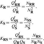(8)

under the constraint N_RS = N⁰_R − 2N_RR − N_R=N⁰_S − 2N_SS − N_S, in which N⁰ are the initial concentrations of single strands. We noticed that Q_R and Q_S computed by the three programs are very close because they use the same algorithm for a single strand (i.e. McCaskill's algorithm). Therefore based on (8), a method can compute equilibrium concentrations correctly only if it computes each individual Q^I accurately. As one can observe in Figure 11, our program has been able to predict OxyS–fhlA complex concentrations accurately, thus we can conclude that our program computes all Q^I accurately.

As mentioned above, the parameters used by our program on this dataset have been manually optimized. Our energy parameters in this experiment are β₁ = 6.6, β₂ = β₂ = 0.1, σ = 0.9, β′₁ = 4.5 and σ′ = 0.9.

4 CONCLUSION AND FUTURE WORK

In this article, we present piRNA, an efficient algorithm to compute a partition function of two interacting nucleic acid strands. Our algorithm considers almost all physically possible secondary structures that do not contain pseudoknots, crossing interactions and ‘zigzag's. In order to specify the free energy of a joint structure established by interacting strands, we extend the standard nearest neighbor single-strand thermodynamic energy model to an energy model for two interacting strands by introducing three new components: (i) hybrid component, (ii) kissing loop and (iii) inter-hybrid loops that are modified versions of hybridization, multi loop and pseudoknot energy models. We verified our algorithm by computing the melting temperature for RNA pairs available in the literature and the equilibrium concentration for OxyS-fhlA complex. In both experiments our algorithm provides high accuracy and outperforms available alternatives.

We computed the melting temperature for RNA pairs in (Diamond et al., 2001; Mathews and Turner, 2002; Xia et al., 1998) (Tables 1–3). On average, the predicted melting temperature by our program is ∼2^○C different from experimental values. Our program is >10^○C more accurate than the alternatives, RNAcofold and UNAFold, on average. It is important to note that RNAcofold and UNAFold both perform poorly in at least one of the three datasets, while our program is consistently accurate across all three datasets. Therefore, neither RNAcofold nor UNAFold is as reliable as our program for melting temperature prediction. In addition, our algorithm is able to compute the OxyS–fhlA complex equilibrium concentrations for wild-type and mutated fhlA accurately. Both RNAcofold and UNAFold predict those equilibrium concentrations to be approximately 0, which does not even roughly follow the experimental measurements.

Although our algorithm is fairly efficient, improving the generality and complexity of our algorithm will be one of our priorities in the near future. In particular, we aim to explore whether it is possible to cover more general interactions without increasing the computational complexity of the algorithm.

Funding: Bioinformatics for Combating Infectious Diseases (BCID) initiative (to H.C.). MITACS Research Grant (to R.S.). Michael Smith Foundation for Health Research Career Award (to S.C.S.). German Research Foundation (DFG grant BA 2168/2-1 SPP 1258), and from the German Federal Ministry of Education and Research (BMBF grant 0313921 FRISYS) (to R.B.).

Conflict of Interest: none declared.

REFERENCES

- Alkan C, et al. RNA-RNA interaction prediction and antisense RNA target search. J. Comput. Biol. 2006;13:267–282. doi: 10.1089/cmb.2006.13.267. [DOI] [PubMed] [Google Scholar]
- Andronescu M, et al. Secondary structure prediction of interacting RNA molecules. J. Mol. Biol. 2005;345:987–1001. doi: 10.1016/j.jmb.2004.10.082. [DOI] [PubMed] [Google Scholar]
- Argaman L, Altuvia S. fhlA repression by OxyS RNA: kissing complex formation at two sites results in a stable antisense-target RNA complex. J. Mol. Biol. 2000;300:1101–1112. doi: 10.1006/jmbi.2000.3942. [DOI] [PubMed] [Google Scholar]
- Bartel BP. MicroRNAs: genomics, biogenesis, mechanism, and function. Cell. 2004;116:281–297. doi: 10.1016/s0092-8674(04)00045-5. [DOI] [PubMed] [Google Scholar]
- Bernhart S, et al. Partition function and base pairing probabilities of RNA heterodimers. Algorithms Mol. Biol. 2006;1:3. doi: 10.1186/1748-7188-1-3. [DOI] [PMC free article] [PubMed] [Google Scholar]
- Brantl S. Antisense-RNA regulation and RNA interference. Bioch. Biophys. Acta. 2002;1575:15–25. doi: 10.1016/s0167-4781(02)00280-4. [DOI] [PubMed] [Google Scholar]
- Busch A, et al. IntaRNA: efficient prediction of bacterial sRNA targets incorporating target site accessibility and seed regions. Bioinformatics. 2008;24:2849–2856. doi: 10.1093/bioinformatics/btn544. [DOI] [PMC free article] [PubMed] [Google Scholar]
- Cao S, Chen S. Predicting RNA pseudoknot folding thermodynamics. Nucleic Acids Res. 2006;34:2634–2652. doi: 10.1093/nar/gkl346. [DOI] [PMC free article] [PubMed] [Google Scholar]
- Diamond J, et al. Thermodynamics of three-way multibranch loops in RNA. Biochemistry. 2001;40:6971–6981. doi: 10.1021/bi0029548. [DOI] [PubMed] [Google Scholar]
- Dimitrov RA, Zuker M. Prediction of hybridization and melting for double-stranded nucleic acids. Biophys. J. 2004;87:215–226. doi: 10.1529/biophysj.103.020743. [DOI] [PMC free article] [PubMed] [Google Scholar]
- Dirks RM, et al. Thermodynamic analysis of interacting nucleic acid strands. SIAM Review. 2007;49:65–88. [Google Scholar]
- Dirks RM, Pierce NA. A partition function algorithm for nucleic acid secondary structure including pseudoknots. J. Comput. Chem. 2003;24:1664–1677. doi: 10.1002/jcc.10296. [DOI] [PubMed] [Google Scholar]
- Gottesman S. Micros for microbes: non-coding regulatory RNAs in bacteria. Trends Genet. 2005;21:399–404. doi: 10.1016/j.tig.2005.05.008. [DOI] [PubMed] [Google Scholar]
- Hannon GJ. RNA interference. Nature. 2002;418:244–251. doi: 10.1038/418244a. [DOI] [PubMed] [Google Scholar]
- Hjalt T, Wagner E. Bulged-out nucleotides in an antisense RNA are required for rapid target RNA binding in vitro and inhibition in vivo. Nucleic Acids Res. 1995;23:580–587. doi: 10.1093/nar/23.4.580. [DOI] [PMC free article] [PubMed] [Google Scholar]
- Kato Y, et al. A grammatical approach to RNA-RNA interaction prediction. Pattern Recognit. 2009;42:531–538. [Google Scholar]
- Landau LD, Lifshitz EM. Statistical Physics. Oxford, UK: Pergamon; 1969. [Google Scholar]
- Markham N, Zuker M. UNAFold: software for nucleic acid folding and hybridization. Methods Mol. Biol. 2008;453:3–31. doi: 10.1007/978-1-60327-429-6_1. [DOI] [PubMed] [Google Scholar]
- Mathews D. Using an RNA secondary structure partition function to determine confidence in base pairs predicted by free energy minimization. RNA. 2004;10:1178–1190. doi: 10.1261/rna.7650904. [DOI] [PMC free article] [PubMed] [Google Scholar]
- Mathews D, et al. Expanded sequence dependence of thermodynamic parameters improves prediction of RNA secondary structure. J. Mol. Biol. 1999;288:911–940. doi: 10.1006/jmbi.1999.2700. [DOI] [PubMed] [Google Scholar]
- Mathews D, Turner D. Experimentally derived nearest-neighbor parameters for the stability of RNA three- and four-way multibranch loops. Biochemistry. 2002;41:869–880. doi: 10.1021/bi011441d. [DOI] [PubMed] [Google Scholar]
- McCaskill J. The equilibrium partition function and base pair binding probabilities for RNA secondary structure. Biopolymers. 1990;29:1105–1119. doi: 10.1002/bip.360290621. [DOI] [PubMed] [Google Scholar]
- Mü#ckstein U, et al. Thermodynamics of RNA-RNA binding. Bioinformatics. 2006;22:1177–1182. doi: 10.1093/bioinformatics/btl024. [DOI] [PubMed] [Google Scholar]
- Nussinov R, et al. Algorithms for loop matchings. SIAM J. Appl. Math. 1978;35:68–82. [Google Scholar]
- Pervouchine D. IRIS: intermolecular RNA interaction search. Genome Inform. 2004;15:92–101. [PubMed] [Google Scholar]
- Puglisi J, Tinoco I. Absorbance melting curves of RNA. Meth. Enzymol. 1989;180:304–325. doi: 10.1016/0076-6879(89)80108-9. [DOI] [PubMed] [Google Scholar]
- Rehmsmeier M, et al. Fast and effective prediction of microRNA/target duplexes. RNA. 2004;10:1507–1517. doi: 10.1261/rna.5248604. [DOI] [PMC free article] [PubMed] [Google Scholar]
- Rivas E, Eddy S. A dynamic programming algorithm for RNA structure prediction including pseudoknots. J. Mol. Biol. 1999;285:2053–2068. doi: 10.1006/jmbi.1998.2436. [DOI] [PubMed] [Google Scholar]
- Seeman N. From genes to machines: DNA nanomechanical devices. Trends Biochem. Sci. 2005;30:119–125. doi: 10.1016/j.tibs.2005.01.007. [DOI] [PMC free article] [PubMed] [Google Scholar]
- Seeman NC, Lukeman PS. Nucleic acid nanostructures: bottom-up control of geometry on the nanoscale. Rep. Prog. Phys. 2005;68:237–270. doi: 10.1088/0034-4885/68/1/R05. [DOI] [PMC free article] [PubMed] [Google Scholar]
- Simmel F, Dittmer W. DNA nanodevices. Small. 2005;1:284–299. doi: 10.1002/smll.200400111. [DOI] [PubMed] [Google Scholar]
- Storz G. An expanding universe of noncoding RNAs. Science. 2002;296:1260–1263. doi: 10.1126/science.1072249. [DOI] [PubMed] [Google Scholar]
- Venkataraman S, et al. An autonomous polymerization motor powered by DNA hybridization. Nat. Nanotechnol. 2007;2:490–494. doi: 10.1038/nnano.2007.225. [DOI] [PubMed] [Google Scholar]
- Wagner E, Flardh K. Antisense RNAs everywhere? Trends Genet. 2002;18:223–226. doi: 10.1016/s0168-9525(02)02658-6. [DOI] [PubMed] [Google Scholar]
- Walton S, et al. Thermodynamic and kinetic characterization of antisense oligodeoxynucleotide binding to a structured mRNA. Biophys. J. 2002;82:366–377. doi: 10.1016/S0006-3495(02)75401-5. [DOI] [PMC free article] [PubMed] [Google Scholar]
- Waterman MS, Smith TF. RNA secondary structure: A complete mathematical analysis. Math. Biosc. 1978;42:257–266. [Google Scholar]
- Xia T, et al. Thermodynamic parameters for an expanded nearest-neighbor model for formation of RNA duplexes with Watson-Crick base pairs. Biochemistry. 1998;37:14719–14735. doi: 10.1021/bi9809425. [DOI] [PubMed] [Google Scholar]
- Yin P, et al. Programming DNA tube circumferences. Science. 2008;321:824–826. doi: 10.1126/science.1157312. [DOI] [PubMed] [Google Scholar]
- Zamore PD, Haley B. Ribo-gnome: the big world of small RNAs. Science. 2005;309:1519–1524. doi: 10.1126/science.1111444. [DOI] [PubMed] [Google Scholar]
- Zuker M, Stiegler P. Optimal computer folding of large RNA sequences using thermodynamics and auxiliary information. Nucleic Acids Res. 1981;9:133–148. doi: 10.1093/nar/9.1.133. [DOI] [PMC free article] [PubMed] [Google Scholar]