Speeding up HMM algorithms for genetic linkage analysis via chain reductions of the state space

Abstract

We develop an hidden Markov model (HMM)-based algorithm for computing exact parametric and non-parametric linkage scores in larger pedigrees than was possible before. The algorithm is applicable whenever there are chains of persons in the pedigree with no genetic measurements and with unknown affection status. The algorithm is based on shrinking the state space of the HMM considerably using such chains. In a two g-degree cousins pedigree the reduction drops the state space from being exponential in g to being linear in g. For a Finnish family in which two affected children suffer from a rare cold-inducing sweating syndrome, we were able to reduce the state space by more than five orders of magnitude from 2⁵⁰ to 2³². In another pedigree of state-space size of 2²⁷, used for a study of pituitary adenoma, the state space reduced by a factor of 8.5 and consequently exact linkage scores can now be computed, rather than approximated.

Contact: dang@cs.technion.ac.il

Supplementary information: Supplementary data are available at Bioinformatics online.

1 INTRODUCTION

Genetic linkage analysis seeks to locate genomic regions that are likely to contain genes that increase the probability of traits such as heredity diseases. The input to such analysis are pedigrees of families that segregate a disease, marker information such as SNP readings, and affection status of some or all family members. The main idea is that markers which are found in the same vicinity on the chromosome are more likely to stay together during meiosis. Thus, based on the topology of the pedigree and the marker readings, it is possible to compute how likely it is for a predisposing gene to be located on the chromosome nearby each of the markers (Elston and Stewart, 1971; Lander and Green, 1987; Lange, 1997; Ott, 1999).

There are several scoring methods commonly used for linkage analysis. They differ in how the scoring function depends on the probability of the possible inheritance patterns in the pedigree. Examples of such functions are S_all, S_pairs and log of odds (LOD) scores (Kruglyak et al., 1996). As the number of such inheritance patterns grows exponentially in the number of markers and roughly in the number of persons in the pedigree, computationally sophisticated methods were proposed for this task. A common structure shared by most exact scoring methods is a hidden Markov model (HMM) (Rabiner and Juang, 1986) backbone, which is in fact a factored HMM with a state space defined by a set of variables called selectors that determine the inheritance pattern in the pedigree (Abecasis et al., 2002; Gudbjartsson et al., 2000, 2005; Ingolfsdottir and Gudbjartsson, 2005; Kruglyak and Lander, 1998; Kruglyak et al., 1995, 1996; Lander and Green, 1987; Markianos et al., 2001). Other techniques based, sometimes implicitly, on Bayesian networks (Lauritzen, 1996; Pearl, 1988) focus on larger pedigrees with fewer measurements (Cottingham et al., 1993; Elston and Stewart, 1971; Fishelson and Geiger, 2002; O'Connell and Weeks, 1995; Silberstein et al., 2006; Sobel and Lange, 1996; Thompson, 1994).

Whenever the pedigree is too complex, and the number of selectors needed to determine the inheritance in the pedigree is too large, current methods can not utilize the HMM backbone, and exact computation of the linkage scores is not computationally feasible. In this article, we describe a method to reduce the state space for HMMs via a partition of the state space into equivalence classes, which consequently reduces the amount of computations needed in these models without sacrificing the exact solution. We specify two conditions a partition needs to satisfy in order to allow for such a reduction, and prove that whenever they hold, computations in the original and the reduced models yield the same results.

A partition which is of particular interest for the HMM used for linkage analysis models is based on reducing chains of individuals in pedigrees where genetic information cannot distinguish among individuals in the chain. In such chains, it is possible to cluster together selector variables that control the inheritance from a founder allele in the pedigree, indicating only if the allele is transmitted to the individual at the end of the chain or, if not, what is the number of selectors that block its inheritance. For r selectors (meiosis), this clustering reduces the state space from 2^r to r + 1 states.

To demonstrate the usefulness of the state-space reduction, we provide several examples of pedigrees in which computations are significantly easier once the reduction is used. For a Finnish family in which two affected children suffer from a rare cold-inducing sweating syndrome (Knappskog et al., 2003), we were able to reduce the state space of the internal inbreeding loop by over 9-folds, and to reduce the state space for the entire pedigree by more than five orders of magnitude from 2⁵⁰ to 2³². For another pedigree, recently used for the study of pituitary adenoma (Vierimaa et al., 2006), we were able to reduce the state space from 2²⁷ to 60 · 2¹⁸, by a factor of more than 8.5. Previously, only approximate scores could be computed for this pedigree on a standard PC and software for exact linkage computations such as Merlin (Abecasis et al., 2002) failed as reported by Albers et al. (2008). Our space reduction enables exact linkage computations and we demonstrate order of magnitude experimental speedups when performing computations across 6000 genomic locations, as used by standard SNP panels for linkage analysis.

2 STATE REDUCTION IN HMMS

Consider an HMM with hidden variables S_i and observed variables X_i, i = 1,…, L (Rabiner and Juang, 1986). The (hidden) state space is the set S of possible values for S_i. The state space is identical for every slot i. The likelihood of data (x₁,…, x_L) for L slots is specified via two main components. The single slot likelihood of data P(x_i|s_i) at slot i given a state s_i for S_i and the transition probabilities P(S_i = s_i|S_i−1 = s_i−1) from a state at slot i − 1 to slot i.

(1)

The time complexity of computing this sum grows quadratically with the size of the state space |S| and linearly in the number of slots L. The time complexity is O(L|S|² + cL|S|) where c is an upper bound for computing the single slot likelihood P(x_i|s_i). We note that in many HMM applications, including linkage analysis, the goal is to compute the marginal probabilities P(S_i|x₁,…, x_L) for all i = 1,…, L rather than to compute the likelihood of data. This task can be completed using the junction-tree algorithm with only twice the computational cost (Lauritzen and Spiegelhalter, 1988). We show experimental results for both tasks, but restrict the discussion to computation of the likelihood to simplify the presentation.

We focus on applications where S is possibly very large such as for linkage analysis where it grows exponentially in, roughly, the number of persons in the pedigree. In such cases, the dominating factor |S|² can be reduced substantially if the state space S can be partitioned into equivalence classes [s] for which the likelihood of data is constant. This effectively changes the sum over the state space at each slot to a sum over equivalence classes. The dominating complexity will now depend on the number of equivalence classes rather than on the number of states in S.

The likelihood is computed for one representative of each equivalence class via

(2)

where the prior for a class [s] is the sum over the priors of its constituent states, namely, P([s]) = ∑_s∈[s]P(s). Note that [s_i] is used to denote the class containing s_i, as in s_i∈[s_i], and also a representative from the class containing state s_i, as in S_i=[s_i].

The equivalence of Equations (1) and (2) stems from two general conditions. Explicating these conditions facilitates the discovery of novel equivalence classes that reduce the computational cost of likelihood computations, as we show for genetic linkage analysis.

Condition I: —

the single-slot likelihood given a hidden state s is equal for all states in the equivalence class [s], namely, P(x_i|s) = P(x_i|s′) for all s and s′ in the same equivalence class. Hence, we can safely define the single-slot likelihood given an equivalence class via P(x_i|[s]) = P(x_i|s).

Condition II: —

denote by P([s]|s′) = ∑_s∈[s]P(s|s′) the transition probability from state s′ to an equivalence class [s]. The condition is that this transition probability does not distinguish between two states in the same equivalence class, namely, P([s]|s′) = P([s]|s″) for all s′ and s″ in the same equivalence class. Hence, we can safely define the transition probabilities between equivalence classes via P([s]|[s′]) = P([s]|s′).

These two natural conditions are sufficient to ensure that Equations (1) and (2) are equivalent due to the following reasoning. We first rewrite the right most sum in Equation (1). The following equality is due to Condition I.

The latter sum is further rewritten,

where the final equality is due to Condition II. Proceeding with these steps over decreasing indices L, L − 1,…, 1 transforms Equation (1) to Equation (2) where in the last step P([s₁]) is set to ∑_s1∈[s1]P(s₁).

3 STATE-SPACE REDUCTION IN FACTORED HMMS

Factored HMMs (Ghahramani and Jordan, 1997) are HMMs in which the hidden variable is a vector S_i = (S_i¹,…, S_i^k) with values drawn from a Cartesian product H₁ × ··· × H_k and with a transition probability defined component by component for i = 2,…, L via

(3)

and for the first slot, P(S₁ = (s₁¹,…, s₁^k)) = ∏_j=1^k P_j(s₁^j). When all the component transition probabilities P_j are equal for all j, we term the resulting HMM a homogeneously factored HMM.

Factored HMMs offer computational benefits when computing the likelihood of data. Ghahramani and Jordan (1997) show how specifying the probabilities P(S_i|S_i−1) via a product as in Equation (3) reduces the time complexity to O(L|S|log|S| + cL|S|). Their algorithm is a special case of bucket elimination (Dechter, 1998). We note that computing the L marginal probabilities P(S_i|x₁,…, x_L) in a factored HMM can be performed with only twice the amount of computations using the junction-tree algorithm (Lauritzen and Spiegelhalter, 1988).

We offer state-space reductions for homogeneously factored HMMs that maintain these benefits and further reduce the computational complexity. For simplicity of notation, we assume that H_i = {0, 1} and so each S_i^j is a binary variable, which we call a selector, and the state-space size is 2^k. The state-space reductions are formed by clustering the selectors and partitioning the states of each cluster so that Conditions I and II are satisfied.

Assuming the choice of clusters is such that Conditions I and II are satisfied, we now explicate how the likelihood of data computations are carried out in the reduced state space, and examine the reduction in time and space complexity of the computation. In particular, starting with Equation (1), we need to show how the computation of each sum is done when the state space is in a factored form. Suppose ℬ = {B₁,…, B_m} is a set of disjoint clusters of all selectors for some slot i with r₁,…, r_m selectors, respectively, and suppose 𝒜 = {A₁,…, A_m} is a set of disjoint clusters of all selectors for the previous slot where S_i^j ∈ B_l iff S_i^j−1 ∈ A_l. Let a_l and b_l denote vectors of zeros and ones of length r_l. Then the final sum in Equation (1), denoted by Σ_L, can be written as follows.

Due to Condition I, we get,

Due to Condition II, the last sum equals P([b_m]|[a_m]). Incorporating these two modifications sequentially for the indices m, m − 1,…, 1 yields

(4)

This sum is carried out right to left, summing over [b_m], then over [b_m−1] and finally over [b₁]. The result is a conditional probability table Σ_L = λ(x_L|[a₁],…, [a_m]). This conditional probability table is carried to the L − 1's sum of Equation (2), and this process is repeated L times, once per slot. Hence, the likelihood depends on the cluster states and not on the states of individual selectors.

We now define a specific choice of clusters and prove that it satisfies Condition II. In the next section, we specify additional domain-specific restrictions in order for this choice to also satisfy Condition I, as needed in order to achieve computational savings. For simplicity, we assume a symmetric transition probability table so that a transition from state 0 at slot i to state 1 and from state 1 to 0 are equal and are denoted by θ_i. Note that the results can be easily extended beyond binary domains H_i = {0, 1} and without assuming symmetric transition probability tables, but this extension is not needed for genetic linkage analysis. A selector can have two complement states: on and off. For a cluster C with r selectors, a state [j] of the reduced state space of C is the equivalence class which contains all vectors of size r that have j entries being on and r − j being off. So, we have c(j, r) = r!/j!(r − j)! vectors in state [j] for j = 0,…, r. This set of r + 1 equivalent classes is called the counting partition.

Theorem 1. —

Let S = (S¹,…, S^k) be a vector of selectors and let 𝒞={C₁,…, C_m} be a set of disjoint clusters with r₁,…, r_m selectors, respectively, in each cluster, where k = ∑_j=1^m r_j. Then a factored HMM in which the hidden variable has values drawn from the Cartesian product [𝒞] = [C₁] × ··· × [C_m], where [C_l] is the set of equivalence classes of cluster C_l generated by using the counting partition, satisfies Condition II.

PROOF. —

To prove that Condition II holds for the counting partition, we consider a single cluster C ∈ 𝒞 with r selectors. The transition probability for switching from a state of C with j positions on to any one state with i positions on is developed below. Let θ be the probability of switching from state on to state off and of switching from state off to state on. The other two transitions have probability 1 − θ. The probability of switching from a state where j selectors are on to the state [i] in which some arbitrary i selectors are on is given by

where t is the number of selectors that are on both in [i] and in the state . Since this formula does not depend on which j selectors are on, it follows that . This is exactly Condition II for one cluster of r selectors. These definitions of the transition probability tables apply separately to each of the clusters C₁,…, C_m. Consequently, the conditional probabilities P([s]|s′) satisfy Condition II via

where c_l is the component of state s for the selectors associated with C_l, and where c_l′ and c_l″ are the components for the selectors C_l of the two equivalent states s′ and s″. ▪

The counting partition reduces the state space of each cluster with r selectors from 2^r to r + 1 states. Thus, the complexity of computing Equation (4) for this partition is the following. Suppose the k selectors are divided into m equally sized clusters each corresponding to k/m selectors and having d = 1 + k/m states. Then summing over [b_m] yields a probability table λ(x_L|[b₁],…, [b_m−1], [a_m]). The next sum yields a table λ(x_L|[a₁],…, [b_m−2], [a_m−1], [a_m]). Finally, the conditional probability table Σ_L = λ(x_L|[a₁], […, [a_m]) is created. Since each λ table has m dimensions, each step involves O(d^m+1) arithmetic operations. This step is repeated m times, and therefore O(md^m+1) arithmetic operations are used. The entire process is repeated L times, once per slot, and so the overall complexity is O(Lm(1 + k/m)^m) where 1 ≤ m ≤ k. For example, if m = k, each cluster contains one selector, the complexity is O(Lk2^k+1) as suggested by Ghahramani and Jordan (1997) and used in all the current HMM-based linkage analysis programs (Kruglyak and Lander, 1998; Markianos et al., 2001). On the other extreme, when all selectors are clustered together, namely m = 1, then the complexity is merely O(L(1 + k)).

Examples of utilizing the counting partition and obtaining significant speed up in real genetic applications are discussed in the next two sections.

4 APPLICATION IN GENETIC LINKAGE ANALYSIS

The purpose of genetic linkage analysis is to score the human genome in such a way that produces high scores for areas that harbor genes that predispose to a disease under study. The means are pedigrees of families that segregate the disease and genetic information such as SNP data measured on individual members of these families. There are various scoring methods for linkage analysis, some are called parametric and some non-parametric, but all scoring methods share the backbone of a common HMM. This HMM is in fact a homogeneously factored HMM and its state space is defined by a set of selectors precisely as discussed in the previous section. The data at slot i are the measurements of the individuals' genetic material at the i-th location.

In this section, we provide the needed background to describe the meaning of the transition probabilities, define precisely the likelihood P(x_i|s_i) of data at slot i given a hidden state and provide clustering methods that generate the state-space reductions via the counting partition as studied in the previous section.

4.1 HMM for linkage analysis

A pedigree is a directed acyclic graph (V, E) with a set V of n vertices of two possible types called male and female and a set of directed edges E ⊆ V × V such that for each vertex v there is at most one directed edge (u, v) for which the type of u is male and at most one edge for which the type of u is female. When a vertex has in-degree 0, it is called a founder. A vertex that is not a founder is called a non-founder. Each vertex in a pedigree is classified either as typed (measured) or untyped (not measured).

Semantically, each vertex in a pedigree represents a person and each directed link represents a parent–child relationship. When a vertex has in-degree 1, it means that one parent is specified in the pedigree and the other is not. A typed vertex represents a person whose genetic material has been measured. Such person is also said to be typed.

Definition. —

A potential descent graph for a pedigree (V, E) is a directed acyclic graph (V′, E′) such that for every vertex v_i ∈ V, there are two vertices m_i (termed the maternal vertex) and p_i (termed the paternal vertex) in V′, and for every edge (v_i, v_j) ∈ E there are two edges in E′ as follows: if the type of vertex v_i is male, then the edges (m_i, p_j) and (p_i, p_j) are in E′ and if the type of vertex v_i is female, then the edges (m_i, m_j) and (p_i, m_j) are in E′. If a vertex v_i ∈ V is typed, then both m_i and p_i are typed and if v_i is not typed then both m_i and p_i are untyped.

Semantically, the meaning of a pair of vertices (m_j, p_j) is the maternally inherited and paternally inherited genetic information of person j at some genomic location. A parent i contributes either m_i or p_i to each child j.

Definition (Sobel and Lange, 1996). —

A descent graph D = (V″, E″) of a potential descent graph (V′, E′) is a subgraph of (V′, E′) such that V″ = V′ and for every pair of edges {(m_i, p_j), (p_i, p_j)} in E′ exactly one is in E″ and for every pair of edges {(m_i, m_j), (p_i, m_j)} in E′ exactly one is in E″. Vertices that are classified as typed in V′ remain typed in V″ and the other remain untyped.

Note that for a pedigree with n non-founders there are 2²ⁿ descent graphs, since there is a binary choice of genetic material twice for every person that is not a founder. For each choice from a pair of edges, we assign a binary variable called a selector whose values are 0 if the first edge from a pair is chosen and 1 otherwise. The vector of selectors, which is called the inheritance vector, can get 2²ⁿ assignments and each assignment s defines a descent graph denoted by D[s]. Each assignment s is called an inheritance state.

Each descent graph specifies how each of the founding alleles is inherited. That is, given a descent graph of a pedigree and an assignments of alleles a = (a₁,…, a_2f) to the maternal and paternal variables of its f founders, every maternal and paternal variable is assigned a specific founding allele. In other words, each descent graph consists of 2f directed trees, two for each founder, called descent trees and each descent tree specifies how one founder allele is assigned to the maternal and paternal vertices that constitute that tree.

A label of a typed person v_i is an unordered pair of letters {a_i, a_j} from a finite set A. An element of A is called an allele. The label is also termed the genotype of person v_i (at some genomic location). The marker data at some genomic location are a vector of genotypes—one for each typed person.

In the case of SNP marker data, there are only two letters in A and hence each label has three options: {{0, 0}, {0, 1}, {1, 1}}. In the case of simple tandem repeats (STR) markers, there are r letters in A and therefore possible labels of the form {a_i, a_j}. If the genotype of a person is (a′, a″) then either its maternal allele is a′ and its paternal allele is a″ or the converse. The marker data are a vector of unordered pairs and does not distinguish which allele is the maternal and which is the paternal. Each typed person v_i adds a constraint on the possible alleles for (m_i, p_i).

Definition. —

A vector of founder alleles a is said to be consistent with marker data x_i and a descent graph D[s] iff x_i can be obtained by inheritance via D[s] from a. This consistency statement is denoted by a ↦ x_i ∧ s.

The HMM for linkage analysis can now be defined as in Sobel and Lange (1996). The likelihood of a marker data vector x_i given a state s of the inheritance vector is specified by

(5)

where P(a) equals the probability of the founders having a vector of founder alleles a = (a₁,…, a_2f). The product form is justified by the common assumption that the founders are random persons from a population and their two alleles are randomly sampled as well (called Hardy–Weinberg equilibrium). As written, this sum is exponential in the number of founders. However, Sobel and Lange (1996) devised an efficient polynomial algorithm for this sum using founder graphs. The transition probabilities are given by

where P_j(s_i^j|s_i−1^j) = θ_i if s_i^j ≠ s_i−1^j. The biological meaning of the statement s_i^j ≠ s_i−1^j is that a recombination has occurred in the j-th meiosis, namely, in one genomic location a maternal allele of a parent is transmitted to a child and in the next location the paternal allele of the same parent is transmitted to the same child.

The specified model is a homogeneously factored HMM and therefore any clustering of the selectors using the counting partitioning satisfies Condition II, as shown in Theorem 1. The remaining challenge is to define clusters that also satisfy Condition I and for this the properties of the likelihood P(x_i|s) [Equation (5)] must be studied in detail.

4.2 Chain reductions

The main idea for identifying useful clusters is to find chains in the pedigree such that either the chain is on, meaning that an allele is transmitted from the start of the chain to its end, or the chain is off, in which case a random allele is transmitted to the end of the chain. Clusters of such chains only depend on the number of selectors that block the transmission of that allele. This idea is made precise as follows.

Definition. —

A chain of length l in a pedigree is a sequence of edges (v_i, v_i+1), i = 1,…, l, such that nodes v₁,…, v_l are each untyped and have one incoming edge and one outgoing edge in the pedigree, and node v_l+1 has one incoming edge (but may or may not be typed and may have any number of children).

A chain of length l in a pedigree translates to a set of 2l edges in the potential descent graph of the pedigree connecting the maternal and paternal nodes of person v_i to the paternal node of person v_i+1 when v_i is a male, and connecting them to the maternal node of v_i+1 when v_i is a female. In the potential descent graph, we define the maternal node m₁ to be the source of the chain if the parent of person v₁ in the pedigree is a female and define the paternal node p₁ as the source, if the parent of person v₁ is a male. Similarly, we define the sink of the chain to be node m_l+1 if person v_l is a female, and define node p_l+1 as the sink, if person v_l is a male.

There is one descent graph in which the source of the chain is connected by a directed path to the sink of the chain. Let S¹,…, S^l be the selectors associated with the l choices of these edges and define an on state as the choice of an edge on the directed path from source to sink, and by off a choice that disconnects this path.

In practice, before searching for chains in a given pedigree, we transform the pedigree to a normalized form by using the following two operations repeatedly until they no longer apply. First, remove an untyped person that has no children. Second, remove an untyped founder that has one child. It can be shown that the likelihood of marker data remains unchanged under these transformations. Furthermore, it can be assumed that the pedigree is specified in a normalized form. This normalization procedure is merely a rule that tells the geneticist when there is no need to add more persons to the pedigree specification, which, in principle, can expand endlessly to various directions. The normalization procedure can create more chains and consequently facilitates larger state-space reductions.

For example, consider Pedigree I depicted in Figure 1 with three typed children D_t, E_u and F_z who are distant cousins. The parents of individuals along the chains D, E and F are not specified in the normalized pedigree.

For each chain C_j, we define a cluster which we denote also by C_j. The cluster C_j consists of the selectors associated with the chain C_j. Such a chain cluster with l selectors can get one of l + 1 values, corresponding to the number of selectors that are on. This reduction is the counting partition, defined in Section 3. The following theorem states that such chain reductions do not change the likelihood of data. The proof is given in the appendix of the Supplementary Material.

Fig. 1.

A normalized pedigree with two founders (A and B) and three typed distant cousins (D_t, E_u and F_z, with genotypes g₁, g₂ and g₃ respectively). The chains D, E and F can be reduced from a collection of selectors to one cluster each with number of states linear in the chain's length. In Pedigree II, the collection of the selectors in the two chains, can be reduced to a single cluster with number of states linear in the sum of lengths of the two chains.

Theorem 2. —

Let S¹,…, Sⁿ be the selectors for a pedigree (V, E) and let C be a chain in (V, E) such that S¹,…, S^l are the selectors associated with the edges of C. Let S^C be a variable with a value equal to the number of selectors S^j that are on for 1 ≤ j ≤ l. Then the likelihood of data can be computed by summing over the states of S^C, S^l+1,…, Sⁿ.

This chain reduction can be repeated for every chain in the pedigree yielding considerable reduction in the state space. For example, the full-inheritance state space of Pedigree I in Figure 1 corresponds to 4 + t + u + z informative meiosis yielding a state space of size¹ N = 2^t+u+z+4. The reduced state space uses the fact that the likelihood of data does not depend on the exact state of the selectors along the chains D, E and F that connect the typed cousins to the two founders, but only on whether they point toward a common ancestor, and if not, how many selectors do not point to the common ancestor. In other words, how many selectors are off. Consequently, for each W-chain, where W ∈ {D, E, F} of length w, it is possible to cluster the w − 1 selectors from W₂ along the chain into a single variable with w states. Thus, the total reduced state space is now N′ = 2⁷ · t · u · z yielding an exponential reduction of the state space.

5 EXPERIMENTAL RESULTS

We demonstrate the power of the state space reduction in factored HMMs for genetic linkage analysis problems via the pedigree depicted in Figure 2. This pedigree was recently used for the study of pituitary adenoma (Vierimaa et al., 2006). Since the state-space size of the pedigree is 2²⁷, exact linkage scores could not be computed and heuristics were used (Albers et al., 2008). Reducing the chains marked in the figure, of lengths 2, 3 and 4, reduces the state space to 2¹⁸ × 3 × 4 × 5 by an overall factor of 8.5. Consequently, exact linkage scores can now be computed, rather than approximated.

Fig. 2.

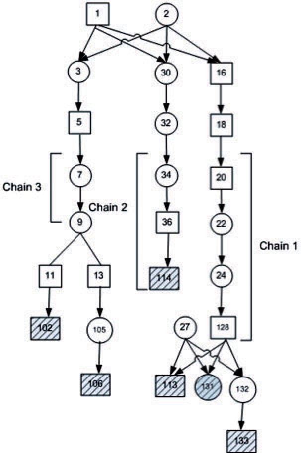
A normalized pedigree used by Vierimaa et al. (2006) for the study of pituitary adenoma. There are six typed individuals in the pedigree that are marked in black stripes. We use chains 1, 2 and 3 to reduce the state space by a factor of 8.5 and speedup computations.

We implemented an algorithm that computes the probabilities P(S_i|data) for every location i, which facilitates the computations of parametric and non-parametric linkage scores. Our implementation supports the factored HMM model for genetic linkage analysis with and without the state-space reduction. We used this software to compare the runtime of computations in the reduced model with the runtime of the original model across 6000 markers, for variable lengths of the chain marked as ‘Chain-1’. Figure 3 shows the runtime in hours for the two models for lengths m = 0,…, 4. For m = 3 and m = 4 the time it takes to perform computations on the original model has been extrapolated from running the software for this model across 150 locations and multiplying by 40. It is evident from the figure that the runtime grows linearly in m in the new model, while it is exponential in m in the original model. The probabilities computed are the same in both models. In addition, Figure 4 plots the runtime of the two models for m = 0 as a function of the number of markers for the computation of the likelihood of data and the inheritance probabilities at all loci given the data. As can be seen, the runtime is linear in the number of markers for both models and the runtime ratio is maintained regardless of the length of the model, as expected. In addition, as predicted from complexity analysis, the runtime of computing probabilities at all loci is twice that of computing the likelihood of data.

Fig. 3.

Runtime comparison for computations using the original model and the reduced state-space model for the pedigree in Figure 2, as a function of the length m of Chain 1.

Fig. 4.

Runtime comparison for computations using the original model and the reduced state-space model for the pedigree in Figure 2 across 6000 markers, where Chain 1 is of length 0.

6 DISCUSSION

In this article, we described two general conditions which, when satisfied, allows one to reduce the state space of HMMs and factored HMMs. We also described when these conditions can be applied to linkage analysis problems which yields a new method for performing exact linkage computations at a potentially reduced cost. In general, when our method reduces the size of the state space it yields a computational savings and, for linkage problems, these savings are exponential.

The computation of exact linkage scores (LOD or non-parametric) in linkage analysis is of great importance. Having an exact linkage scores provides researchers confidence to proceed with the often expensive and time-consuming fine-mapping process. The use of approximate linkage score methods typically yields no guarantees or loose bounds that do not enable a researcher to draw conclusions regarding the linkage score. In addition, for stochastic-based Monte Carlo techniques, researcher must rely on approximate tests of convergence.

Our state-space reduction method does not yield a computational benefit for all pedigrees, but, as we describe herein, it can yield a significant reduction of the computational cost. This reduction can be crucial for some pedigrees, turning a previously intractable computation into one that is tractable, and beneficial for others. In addition, the identification of the potential cost savings of our method is easy and can even be done by manual inspection of the pedigree.

The general idea of collapsing states into equivalence classes is a natural one, yet its realization in genetic linkage analysis is far less obvious because the standard way to represent linkage problems uses redundant selector variables. Identifying these redundancies and using them to speed computations is one of our novel contributions.

In our method, we focus on reducing the state space by the quotient of the subspace that arise from chains in a pedigree, where no genetic information is available for individuals on the chain. For a chain that consists of r selectors the state space reduces from 2^r to r + 1. Although such chains are the most common structure that enables the space reduction, there are cases when more reductions are possible such as combing two chains together. Consider Pedigree II depicted in Figure 1 within the dashed rectangle with two affected distant cousins D_t and E_u. Here, the full-inheritance state-space size equals N = 2^t+u+2. In the reduced state space, the likelihood of data depends only on the combined number of selectors that are off in chains D and E combined. Consequently, it is possible to cluster the t + u selectors into a single counting variable with t + u + 1 states. The total reduced state space is now N′ = 2² · (t + u + 1) yielding an exponential reduction of the state space and, for this example, an algorithm that grows quadratically in the number of persons in the chains and linearly in the number of markers. Without combining the two chains, the reduction would be smaller yielding a total reduced state space of N″ = 2² · (t + 1)(u + 1).

As another example consider the internal inbreeding loop of the family shown in Figure 5 which connects the two parents of the affected individuals. We retain four selectors for the two affected children and one selector for a child of the common founder. All other 13 selectors for the two chains are replaced with a single counting variable with 14 states that replaces both chains, rather than having one cluster per chain. The state space reduces from 2¹⁸ = 252, 144 to merely 14 × 2⁵ = 448, by a factor of 64/7. When considering contracting chains in the entire pedigree, the total state space dropped from 2⁵⁰, which is completely infeasible, to a state space of 2³², a reduction of more than five orders of magnitude.

Fig. 5.

The Finnish family studied by Knappskog et al. (2003), which includes two affected individuals that suffer from cold-inducing sweating syndrome (marked in black).

HMMs and factored HMMs are widely used in various applications, thus speeding up common algorithms in these models, as done via the state-space reduction, can be proved useful for other domains as well. We note that the challenge in applying the reduction to other domains lies in finding a suitable partition of the state space, which satisfies Conditions I and II. Once these conditions are satisfied, the computational savings are automatic and do not require a special analysis. Finally, we note that our state-space reductions are also immediately applicable to other methods for linkage analysis such as Silberstein et al. (2006), Sobel and Lange (1996) and Thompson (1994).

REFERENCES

- Abecasis GR, et al. Merlin-rapid analysis of dense genetic maps using sparse gene flow trees. Nat. Genet. 2002;30:97–101. doi: 10.1038/ng786. [DOI] [PubMed] [Google Scholar]
- Albers C, et al. Multipoint approximations of identity-by-descent probabilities for accurate linkage analysis of distantly related individuals. Am. J. Hum. Genet. 2008;82:607–622. doi: 10.1016/j.ajhg.2007.12.016. [DOI] [PMC free article] [PubMed] [Google Scholar]
- Cottingham RW, et al. Faster sequential genetic linkage computations. Am. J. Hum. Genet. 1993;53:252–263. [PMC free article] [PubMed] [Google Scholar]
- Dechter R. Bucket elimination: a unifying framework for probabilistic inference. In: Jordan MI, editor. Learning in Graphical Models. Kluwer Academic Press; 1998. pp. 75–104. [Google Scholar]
- Elston R, Stewart J. A general model for the analysis of pedigree data. Hum. Hered. 1971;21:523–542. doi: 10.1159/000152448. [DOI] [PubMed] [Google Scholar]
- Fishelson M, Geiger D. Exact genetic linkage computations for general pedigrees. Bioinformatics. 2002;18(Suppl. 1):S189–S198. doi: 10.1093/bioinformatics/18.suppl_1.s189. [DOI] [PubMed] [Google Scholar]
- Ghahramani Z, Jordan M. Machine Learning. MIT Press; 1997. Factorial hidden Markov models. [Google Scholar]
- Gudbjartsson DF, et al. Allegro, a new computer program for multipoint linkage analysis. Nat. Genet. 2000;25:12–13. doi: 10.1038/75514. [DOI] [PubMed] [Google Scholar]
- Gudbjartsson D, et al. Allegro version 2. Stat. Sci. 2005;37:1015–1016. doi: 10.1038/ng1005-1015. [DOI] [PubMed] [Google Scholar]
- Ingolfsdottir A, Gudbjartsson D. Genetic linkage analysis, algorithms and their implementation. Trans. Comput. Syst. Biol. 2005:123–144. [Google Scholar]
- Knappskog P, et al. Cold-induced sweating syndrome is caused by mutations in the CRLF1 Gene. Am. J. Hum. Genet. 2003;72:375–383. doi: 10.1086/346120. [DOI] [PMC free article] [PubMed] [Google Scholar]
- Kruglyak L, Lander E. Faster multipoint linkage analysis using Fourier transform. J. Comput. Biol. 1998;5:1–7. doi: 10.1089/cmb.1998.5.1. [DOI] [PubMed] [Google Scholar]
- Kruglyak L, et al. Rapid multipoint linkage analysis of recessive traits in nuclear families including homozygosity mapping. Am. J. Hum. Genet. 1995;56:519–527. [PMC free article] [PubMed] [Google Scholar]
- Kruglyak L, et al. Parametric and nonparametric linkage analysis: a unified multipoint approach. Am. J. Hum. Genet. 1996;58:1347–1363. [PMC free article] [PubMed] [Google Scholar]
- Lander E, Green P. Construction of multilocus genetic maps in humans. Proc. Natl Acad. Sci. 1987;84:2363–2367. doi: 10.1073/pnas.84.8.2363. [DOI] [PMC free article] [PubMed] [Google Scholar]
- Lange K. Mathematical and Statistical Methods for Genetic Analysis. New York: Springer; 1997. [Google Scholar]
- Lauritzen SL, Spiegelhalter DJ. Local computations with probabilities on graphical structures and their application to expert systems (with discussion) J. R. Stat. Soc. Ser. B. 1988;50:157–224. [Google Scholar]
- Lauritzen SL. Graphical Models. Oxford: Oxford University Press; 1996. [Google Scholar]
- Markianos K, et al. Efficient multipoint linkage analysis through reduction of inheritance space. Am. J. Hum. Genet. 2001;68:963–977. doi: 10.1086/319507. [DOI] [PMC free article] [PubMed] [Google Scholar]
- O'Connell J, Weeks D. The VITESSE algorithm for rapid exact multilocus linkage analysis via genotype set-recoding and fuzzy inheritance. Nat. Genet. 1995;11:402–408. doi: 10.1038/ng1295-402. [DOI] [PubMed] [Google Scholar]
- Ott J. Analysis of Human Genetic Linkage. Baltimore, MD: Johns Hopkins University Press; 1999. [Google Scholar]
- Pearl J. Probabilistic Reasoning in Intelligent Systems. San Francisco, CA: Morgan Kaufmann; 1988. [Google Scholar]
- Rabiner LR, Juang BH. An introduction to Hidden Markov models. IEEE ASSP Mag. 1986:415. [Google Scholar]
- Silberstein M, et al. Online system for faster multipoint linkage analysis via parallel execution on thousands of personal computers. Am. J. Hum. Genet. 2006;78:922–935. doi: 10.1086/504158. [DOI] [PMC free article] [PubMed] [Google Scholar]
- Sobel E, Lange K. Descent graphs in pedigree analysis: applications to haplotyping, location scores, and marker sharing statistics. Am. J. Hum. Genet. 1996;58:1323–1337. [PMC free article] [PubMed] [Google Scholar]
- Thompson EA. Monte Carlo likelihood in genetic mapping. Stat. Sci. 1994;9:355–366. doi: 10.1098/rstb.1994.0073. [DOI] [PubMed] [Google Scholar]
- Vierimaa O, et al. Pituitary Adenoma predisposition caused by germline mutations in the AIP Gene. Science. 2006;312:1228–1230. doi: 10.1126/science.1126100. [DOI] [PubMed] [Google Scholar]