PICKY: a novel SVD-based NMR spectra peak picking method

Abstract

Motivation: Picking peaks from experimental NMR spectra is a key unsolved problem for automated NMR protein structure determination. Such a process is a prerequisite for resonance assignment, nuclear overhauser enhancement (NOE) distance restraint assignment, and structure calculation tasks. Manual or semi-automatic peak picking, which is currently the prominent way used in NMR labs, is tedious, time consuming and costly.

Results: We introduce new ideas, including noise-level estimation, component forming and sub-division, singular value decomposition (SVD)-based peak picking and peak pruning and refinement. PICKY is developed as an automated peak picking method. Different from the previous research on peak picking, we provide a systematic study of the proposed method. PICKY is tested on 32 real 2D and 3D spectra of eight target proteins, and achieves an average of 88% recall and 74% precision. PICKY is efficient. It takes PICKY on average 15.7 s to process an NMR spectrum. More important than these numbers, PICKY actually works in practice. We feed peak lists generated by PICKY to IPASS for resonance assignment, feed IPASS assignment to SPARTA for fragments generation, and feed SPARTA fragments to FALCON for structure calculation. This results in high-resolution structures of several proteins, for example, TM1112, at 1.25 Å.

Availability: PICKY is available upon request. The peak lists of PICKY can be easily loaded by SPARKY to enable a better interactive strategy for rapid peak picking.

Contact: mli@uwaterloo.ca

1 INTRODUCTION

Nuclear magnetic resonance (NMR) protein structure determination remains a costly and laborious process. Typically, it takes an experienced spectroscopist weeks or months for a target protein. Currently, most NMR groups follow the standard process, proposed by Wüthrich (1986), which includes data collection, data processing, peak picking, resonance assignment nuclear Overhauser enhancement (NOE) peak assignment and finally, structure calculation. This process is designed according to the basic assumption of NMR structure determination: the 3D structure of the target protein can be uniquely determined, if enough proton–proton distance constraints are provided. Therefore, the entire process works in the following manner: (i) the peak picking step analyzes the resonance spectra, and extracts the chemical shift values; (ii) the resonance assignment step assigns the chemical shift values to atoms; (iii) the NOE peak assignment step identifies the NOE peaks and generates distance constraints according to the resonance assignments; and (iv) the structure calculation step takes distance constraints into consideration, and iteratively generates structures while simultaneously satisfying as many distance constraints as possible.

Automating this entire NMR structure determination process can provide a powerful tool for high-throughput structural genomics, and mitigate costs substantially (Güntert, 2009; Williamson and Craven, 2009). Clearly, peak picking is a prerequisite for all the other steps. Peak picking is a well-known ‘tricky’ step in the NMR structure determination process (Altieri and Byrd, 2004). In a d-dimensional spectrum, a signal, which is often referred to as a ‘peak’, represents a group of d nuclei that can be coupled through bonds (scalar coupling) or through space (spin–spin coupling). In the frequency domain, the coordinate of each dimension of the peak denotes the chemical shift value of the corresponding nucleus. Thus, the task of peak picking is to identify all the signals in an NMR spectrum, such as ¹⁵N-HSQC, HNCO, HNCA, CBCA(CO)NH, HNCACB, ¹⁵N-edited NOESY and TOCSY. Peak picking has been investigated for about 20 years. A variety of techniques, such as neural networks (Carrara et al., 1993; Corne and Johnson 1992), Bayesian methods (Antz et al., 1995; Rouh et al., 1994), three-way decomposition (Korzhnev et al., 2001; Orekhov et al., 2001), and spectrum- and peak property-based methods (Garret et al., 1991; Johnson and Blevins, 1994; Kleywegt et al., 1990; Koradi et al., 1998), have been developed to identify peaks.

AUTOPSY (Koradi et al., 1998) is one of the most well-known peak picking programs. It differs from previous methods in that not only are the data points around a potential peak taken considered, but also further data points, near the local maximum, are taken into account. Given a spectrum, AUTOPSY first estimates the noise level, which is modeled as the sum of a global base noise and an additional local noise. After all the data points that have intensities lower than the noise level are removed, AUTOPSY applies a ‘flood fill’ algorithm to decompose the remaining data points into connected regions. The easily separable peaks are first identified by considering the symmetry and peak shape properties. Lineshapes are then extracted from these peaks. The underlying mathematical assumption is that a well-separable peak shape (a 2D or 3D intensity matrix) can be approximated by the outer product of 1D lineshapes (a 1D intensity vector) times an intensity matrix. For resolving overlapping peaks, AUTOPSY then clusters lineshapes of the separated peaks. In a region with possible overlapping peaks, AUTOPSY tries to interpret this region by a linear combination of all the potential ‘layers’, each of which is constructed from different combinations of lineshapes that overlap with that region. Finally, integration, symmetrization and filtering modules are called to refine the peak lists.

Later, Orekhov et al. (Korzhnev et al., 2001; Orekhov et al., 2001) proposed a multi-dimensional NMR spectra interpretation method, MUNIN, which can only be applied to a 3D or higher dimensional NMR spectra. The idea of MUNIN is similar to that of AUTOPSY: both are based on the assumption that the spectra can be interpreted by a linear combination of different ‘layers’, each of which is the outer product of 1D lineshapes. However, instead of solving this multi-layer problem in each separated region, which AUTOPSY does, MUNIN deals with the entire spectrum. Thus, each ‘layer’ of the MUNIN method might contain several peaks. Also, it is very likely that several such ‘layers’ are required to describe a single peak. MUNIN has some advantages over AUTOPSY; for example, MUNIN can be applied to frequency- or time-domain data, and does not depend on any assumptions about the lineshapes of the peaks. It is worth noticing that MUNIN is not a peak picking method, but it can have a straightforward add-on module for processing the results of decomposition.

Resonance assignment is not the only step in the NMR structure determination process that requires highly accurate peak picking results. The performance of the NOE peak assignment step also depends on peak picking. NOE peak picking problem is easier than multi-dimensional spectra peak picking, because the resonance assignment information is given as the input for NOE peak picking, which can greatly reduce the chance of picking artifacts. Consequently, NOE peak picking method is usually combined with the iterative NOE peak assignment and structure calculation part. For instance, ATNOS (Herrmann et al., 2002) incorporates NOE peak picking and assignment into structure calculation, and refines both sides simultaneously.

Very little progress has been made on peak picking. Currently, NMR labs do not mainly use any automated peak picking software. Both AUTOPSY and MUNIN were tested on only one 2D/3D ¹⁵N-edited NOESY spectrum in their papers. AUTOPSY cannot be successfully run on any of our experimental spectra by its default parameters, and MUNIN is not publicly available. Regarding all of these impediments: peak picking in the NMR community is accomplished manually, and sometimes semi-automatically with the help of assistant software such as SPARKY (Goddard and Kneller, 2007) and NMRView (Johnson and Blevins, 1994), which can achieve restricted peak picking, when the chemical shift values are given. This is a substantial road block to automated NMR protein structure determination.

In this article, we propose a novel peak picking method, PICKY. PICKY adapts a brand new noise estimation method to efficiently estimate the noise. A component forming algorithm is then applied to divide the spectra into components, which is similar to the idea used in AUTOPSY, and a novel merging method is developed to merge some components. Singular value decomposition (SVD) is employed, for the first time, to decompose each component and get the initial peak lists. Finally, a multi-stage refinement procedure is applied to refine the initial peak lists. The performance of PICKY is evaluated on a comprehensive benchmark set containing 32 2D and 3D spectra from eight proteins. To the best of our knowledge, this is the first systematic study of a peak picking method. PICKY demonstrates an average of 88% recall and 74% precision. PICKY is further tested by combining with several existing automated programs to determine the high-resolution structures of several proteins. One such example, TM1112, is shown in this article, with the final structure 1.25 Å RMSD to the native structure.

2 METHODS

2.1 Method outline

PICKY consists of four sequential steps:

• Noise-level estimation: The noise is assumed to be Gaussian and uniform. By estimating an accurate value for the noise level, most of the noisy data points can be easily filtered out.

• Forming and sub-dividing the components: After the elimination of the noisy points, a spectrum looks like a set of discrete components. All the points within each component are identified. Also, the large components are further divided into several new sub-components. Based on the points on the border of the new sub-components, some of them merge again.

• Peak picking: In this step, each component is decomposed into an element-wise product of a set of lineshapes (equal to the dimension of the spectrum) by SVD. Then these lineshapes are searched for local maxima, i.e. peaks.

• Peak pruning and refinement: Not every picked peak is a real peak. An acceptable peak should satisfy a set of constraints. The algorithm does not give up on peaks that fail to satisfy the constraints, rather it attempts to relocate and discover new potential peaks based on such failing peaks. Also, some peaks are omitted by the cross-referencing between the different spectra or by signal-to-noise ratio (SNR) of the peaks.

2.2 Noise-level estimation

To accurately filter the noise, we propose a novel noise-level estimation method. There are several sources of noise in NMR spectra, including measurement noise, water bands and artifacts. For example, water bands affect only a small part of the spectra. Thus, Koradi et al. (1998) considers a local noise in AUTOPSY. The problem is that for computing the noise variance in a small area, containing only a few points, the estimation is inaccurate, since the variance of estimated noise is reversely proportional to the number of used points. Here, a uniform Gaussian noise throughout the spectrum is considered. Each point in the spectrum can be written as

(1)

where s_i represents the observed intensity, t_i represents the actual intensity and η_i∼N(0, σ²_η) represents the i.i.d white Gaussian noise, the desired value for calculation. To estimate the noise variance σ²_η, the actual intensity is predicted for each point. At first, it is assumed that the actual intensity of each point can be estimated acceptably from the intensities of the neighbors. The neighbor set, N, is defined as the set of all the direct neighbors of a particular point, i.e. all the points where their indices in all dimensions differ by at most one. In a d-dimensional spectrum, each point has 3^d − 1 such neighbors. For example, in 2D and 3D spectra, the number of direct neighbors (n=|N|) is 8 and 26, respectively.

The noise sample at each point is estimated by

(2)

(3)

where in Equation (3),

(4)

is the true density estimation error and is assumed to have a much smaller variance than that of σ²_η. ε_i is independent from noise samples; furthermore noise samples are also independent from each other, so one can write

(5)

Usually, NMR spectra peaks are smooth, and so the estimation error variance σ²_ε is negligible. After is computed, all the samples are again examined and omitted, if . The outlier threshold, O_TH, is set to 5 by default, since only about 0.000029% of the values are expected to be at least five SDs away from the mean. Then, σ_η² is computed again by using the new, cleaner samples as .

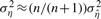After the noise variance is calculated, all the points with absolute values of the observed intensities, less than the noise threshold (N_TH), times the SD of noise (|s_i| <N_TH × σ_η), are omitted (the intensities are set to 0). If the spectrum is supposed to contain only positive intensities, such as the CBCA(CO)NH spectrum, all the negative points are discarded (the intensities are set to 0).

2.3 Forming components

After the filtration of the noisy samples, only a low percentage of the points exhibit non-zero intensities. The spectrum consists of several separate clusters of high-intensity points. Each of these clusters is identified and labeled as a connected component by applying a modified version of the flood-fill algorithm. The algorithm iteratively classifies a point as in the same component as its neighbors (if its neighbors have been already assigned), and forms a new component, otherwise. The component forming algorithm generates hundreds of components, especially for 3D components, and many of them are only a small group of noisy samples which have not been completely eliminated by the noise filtration step. As a result, the components that have fewer than 3^d − 1 points are discarded. Another problem is that some of the components are significantly large. For example, in 2D spectra, such as ¹⁵N-HSQC, several overlapping peaks can form a large component.

The large components are further divided into sub-components. For all of the components, their local maxima are found in a rigorous manner, i.e. each local maximum should be larger than all its first and second tier neighbors. A component is considered large, if it has more than one local maximum. The subdivision is conducted according to the algorithm defined in AUTOPSY (Koradi et al., 1998): each local maximum is labeled with a unique number, and then all of its direct neighbors are labeled with the same number and pushed into a priority queue (PQ). PQ is a list of points which are sorted in terms of their intensities from the highest to the lowest. For the entire algorithm, only the points that have been already assigned with a sub-component index can be pushed into PQ. According to the definition of local maxima, the distance between any two local maxima is at least two data points, and there is no conflict in assigning labels to the neighbors at the beginning of the algorithm. Then, each point in PQ is popped out in the order of its intensity. All the neighbors of this point, which have not been assigned any index, are assigned by this point's index, and then pushed into PQ. This process stops when PQ is empty. It can be easily proved that this sub-division algorithm can detect the border of two components within one data point shift from the optimal solution (proof not shown here).

In AUTOPSY (Koradi et al., 1998), the number of data points within each sub-component is used as the criterion of merging them. An alternative way is to analyze the points on the border of two sub-components. If the intensity of those points is negligible, compared with the intensities of the two corresponding local maxima, there is no need to merge again; otherwise, it means the two potential peaks are highly overlapped, and thus, they should merge again. Thus, if the ratio defined in (6) is larger than merge threshold (M_TH), then the two sub-components merge and a larger sub-component is created.

(6)

where B_i,j is the set of points on the border of sub-components i and j, and m_i and m_j are the intensities of the corresponding local maxima, respectively. M_TH is set to 1/2 in PICKY. For a large component that contains more than two local maxima, this process is applied on each pair of connected local maxima.

2.4 Peak picking

The primary goal of peak picking is to identify real peaks with the highest accuracy, and ignore the false peaks, such as those from water bands or artifacts. The core assumption is the same as that in Koradi et al. (1998), Orekhov et al. (2001) and Korzhnev et al. (2001), where each component that may contain peaks can be approximated as the outer product of the d lineshapes. For example, each 2D component, P ∈ ℝ^p×q, can be approximated by

(7)

where u ∈ ℝ^p×1 and v ∈ ℝ^q×1 are column vectors, called lineshapes, and ⊗ denotes the outer product. Likewise, a 3D 𝒫 ∈ ℝ^p×q×r component is a tensor that can be accurately expressed as

(8)

where u ∈ ℝ^p×1, v ∈ ℝ^q×1 and w ∈ ℝ^r×1 are the column vectors.

If the lineshapes can be predicted accurately, they can be searched for local extrema, considerably reducing the possibility of picking false positive peaks, compared with searching the whole component directly. Here, for 2D spectra, SVD is adopted for component decomposition, and for higher dimensional spectra, higher order SVD (HOSVD) is used. To the best of our knowledge, this is the first time that SVD is applied to solve the peak picking problem.

2.4.1 Matrix decomposition

If SVD is applied to the 2D component, P (Stewart, 1993), then

(9)

where U ∈ ℝ^p×p=(u₁,…, u_p) and V ∈ ℝ^q×q=(v₁,…, v_q) are unitary matrices containing left and right singular vectors, respectively. Singular vectors are orthonormal, i.e.

(10)

and the same holds for v_j. Σ ∈ ℝ^p×q is a matrix with non-negative elements on the diagonal, and zero, elsewhere. The diagonal elements (σ_i≥0) are called singular values and, at most, ℓ of them can be non-zero, where ℓ≤(p, q) is the rank of P. It is assumed that the singular values are sorted non-increasingly. A rank-k approximation of P is then defined as

(11)

It can be shown that P^(k) is the optimal rank-k approximation (Stewart, 1993), i.e. if the approximation error is defined as the Frobenius norm of P−P^(k) such that

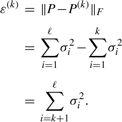(12)

Then, ε^(k) is the minimum of all the rank-k approximations. For the rank-ℓ approximation, ε^(ℓ) is zero or P^(ℓ)=P. Consequently, adding more singular values and their corresponding singular vectors reduces the approximation error. However, if the ratio

(13)

is close to one, the rank-1 approximation (P⁽¹⁾) is accurate enough, particularly, if the P elements are noisy, one can conclude that the small singular values are due to noise, and discarding them can reduce the noise level. For PICKY, after the noisy points filtering and component forming, all the components are quite small and contain either a single strong peak or several highly overlapping peaks. The nature of SVD makes it capable of handling such components, i.e. for almost all the components, R is higher than 0.8, therefore, all other singular values correspond to random noise or contain little information. Figure 1 depicts a component of two highly overlapping peaks. Figure 1b represents the reconstruction of Figure 1a by the vectors, corresponding to the largest singular value. It is clear that Figure 1b is a near-perfect approximation which not only discovers all the potential peaks, but also eliminates the random noise. Thus, for most cases, a rank-1 approximation results in an accurate approximation. In other words, the lineshapes found by SVD are reliable enough to be searched for the possible locations of the peaks, because the lineshapes demonstrate the inherent characteristics of the component, while reducing the noise.

Fig. 1.

Noise reduction using SVD for a 2D component in the ¹⁵N-HSQC spectrum: (a) the original component of two highly overlapping peaks, (b) the reconstruction of (a) by the vectors, corresponding to the largest singular value.

If the singular values are non-degenerate, then their corresponding singular vectors are unique up to the sign, i.e. if u_i and v_i are singular vectors, then −u_i and −v_i produce the same results.

2.4.2 Tensor decomposition

Many informative protein NMR spectra have more than two dimensions, and the standard SVD algorithm cannot be applied. There are several methods for tensor decomposition. By using the Tucker model, a 3D Tensor can be decomposed as follows (Tucker, 1964):

(14)

where s_ijk are the elements of the all-orthogonal intensity tensor 𝒮 with the same dimensions as 𝒫. HOSVD is a generalization of 2D SVD to higher dimensions. HOSVD can be used to decompose 𝒫 as in (14) (De Lathauwer et al., 2000).

Another approach is to decompose 𝒫 by canonical decomposition, as shown in (15) where f is the number of components. The parallel factor analysis (PARAFAC) (Harshman, 1970), which is also called the canonical decomposition (CONDECOMP) (Carroll and Chang, 1970), can be employed for canonical decomposition. Therefore,

(15)

In order to choose the best approach, the Frobenius norm is used for the real three-way tensors and is defined in De Lathauwer et al. (2000) as:

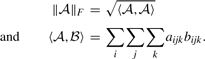(16)

The Frobenius norm of each error tensor is defined as ℰ=‖𝒫−𝒫⁽¹⁾‖_F, where 𝒫⁽¹⁾ consists of only one term of (14) or (15). For the sake of comparison, the term with the smallest normalized error tensor norm (‖ℰ‖_F/‖𝒫‖_F) is chosen which is not noticeably different when tried on real examples. Since HOSVD is very fast and based on widely available numerically stable SVD, it is selected for decomposing the components.

2.5 Peak refinement

The initial list of picked peaks contains many false peaks, that makes them practically useless. Thus, peak refinement is applied to the initial peak lists. Peak refinement is achieved in three steps: peak pruning, cross-referencing and intensity-based filtering. In the peak pruning step, each peak is examined independently and suspicious peaks are removed, and new potential peaks are recovered. Then, the peaks from the spectra, which share some of the common nuclei are cross-referenced to remove the false peaks. Finally, low-intensity peaks are removed.

2.5.1 Peak pruning

An acceptable peak should be larger (or smaller if the component corresponds to a negative-intensity peaks) than its local neighborhood. Each peak's intensity is thus compared with the first and second tier neighbors, i.e. 5^d − 1 points. If a peak fails to satisfy this requirement, a recursive procedure is adopted to change the peak location to achieve satisfaction. It is possible that the final location has been already picked. In this case, the relocated peak is removed. Note that some potential peaks which are not detected by SVD can be recovered in the process.

2.5.2 Peak cross-referencing

After peak pruning, the false peaks are removed by cross-referencing, if the spectra, sharing some common nuclei, are available. For example, the ¹⁵N-HSQC spectrum contains some peaks from the side chains of amino acids such as Asn and Trp. These peaks are removed by cross-referencing them to (N, H^N) chemical shifts of HNCO. If the HNCO spectrum is not available, HNCA is used and so on. The objective is to compare the ¹⁵N-HSQC peaks with the most sensitive available spectrum. After filtering the ¹⁵N-HSQC, its peaks are used to, first, compensate for the shifts in (N, H^N) values of all the NH-based spectra. Then, if the (N, H^N) value of a peak in these spectra does not correspond to any peak in ¹⁵N-HSQC, this peak will be discarded.

2.5.3 Intensity-based filtering

It is assumed that good peaks have high intensities such that the reliability of each peak is defined as the ratio of its intensity to the estimated SD of the noise. After pruning the problematic peaks, in the spectra that the number of expected peaks is previously known (N_r), the remaining peaks are sorted according to their intensities. Then, only K · N_r of them are kept, where K ≥ 1. For example, in the HNCA spectrum of a protein with n residues, an ideal case should be at most 2n − 1 peaks corresponding to the C_α nuclei. K can be set arbitrarily, but as a rule of thumb, K = 1.2 is used for PICKY. When the number of the expected peaks is not known, such as in ¹⁵N-edited NOESY, then the peaks with reliability values below a certain threshold (R_TH) are discarded. R_TH is set to 25 by default.

3 RESULTS

3.1 Peak picking accuracy on raw spectra data

There are two traditional accuracy measures that can provide insight into the accuracy of peak picking: the recall value or the measure of completeness, the ability to discover true peaks; and the precision value or the measure of exactness, the ability to reject false peaks. Assume that in a given spectrum, there are N_r true peaks and a peak picking method picks N_o peaks, where T_p of them are true peaks. Then, recall and precision are defined as recall = T_P/N_r and precision = T_P/N_o, respectively. Apparently, there is a trade-off between recall and precision. For instance, if the peak picking criteria are loose, the recall is high but a large number of false peaks pass through the filter, and result in a low precision.

PICKY's performance is evaluated on 32 spectra of eight proteins from Donaldson's lab at York University and Arrowsmith's lab at the University of Toronto. All the data are noisy raw spectra in the frequency domain, taken by NMR spectrometers from these two labs. In Table 1, the first four proteins, TM1112, YST0336, RP338 and ATC1776, are provided by Arrowsmith's lab, and the other four, COILIN, VRAR, HACS1 and CASKIN, are from Donaldson's lab. Since the peak lists that are manually picked by these experienced spectroscopists are not always available for all these spectra, and it is very common that spectroscopists sometimes do not pick some of the obvious peaks or fail to pick some highly overlapping or buried-in-noise peaks, we generate ‘ideal peak lists’ as the ‘correct answer’, based on the final manually assigned chemical shift table, established by these labs, to fairly compare the PICKY peaks. For example, for residue i of a target protein, a peak for ¹⁵N-HSQC at position (N_i, H^N_i) and a peak for HNCO at positions (N_i, H^N_i, C_i−1) are generated, where N_i, H^N_i and C_i−1 are experimentally assigned chemical shift values of backbone N and H^N atoms for residues i, and a chemical shift value of the backbone C atom for residue i − 1, respectively.

Table 1.

The performance of PICKY on the 32 spectra of eight target proteins (percentile)

Protein	Length	15N-HSQC	HNCO	HNCA	CBCA(CO)NH	HNCACB	Average
TM1112	89	96/89	–	93/88	98/88	91/83	94/87
YST0336	146	91/84	96/79	84/79	86/69	–	89/76
RP3384	64	94/86	100/82	85/70	91/76	–	93/79
ATC1776	101	78/82	89/73	79/75	78/66	–	81/74
COILIN	98	97/70	97/58	–	86/54	78/54	90/59
VRAR	72	87/93	89/84	–	83/71	69/72	82/80
HACS1	74	95/67	94/62	–	94/61	82/52	91/61
CASKIN	67	100/93	85/72	–	91/68	70/75	86/77
Average	–	92/83	93/73	85/78	89/69	78/67	88/74

The first and second columns show target protein names and lengths, respectively. Starting from the third column, for each spectrum of each protein, recall/precision values are listed.

Figure 2 illustrates the PICKY performance on the ¹⁵N-HSQC spectrum of YST0336. The original spectrum is a challenging one, because it contains a huge and crowded region which contains many potential peaks. After PICKY's noise filtering, only about 2% of the data points remain. PICKY then forms components, picks peaks, and refines these peaks by peak pruning, cross-referencing and intensity filtering. It can be seen that most of the overlapping peaks are found, whereas some obvious peaks are eliminated in the refinement process (most of which are caused by histidine-tags and side chains).

Fig. 2.

Illustration of PICKY performance on the 2D ¹⁵N-HSQC spectrum of YST0336. All the data points with intensities >1.5 × 10⁵, which is automatically determined by PICKY, are set to grey. Peaks are shown by the black dots. Some strong peaks, caused by side chains, are filtered by cross-referencing.

It is indicated in Table 1 that PICKY achieves 100% recall on 2 out of 32 spectra,>85% recall on 22 out of 32 spectra, while >85% precision on 6 spectra. The underlying reason for this difference between recall and precision is the way the intensity filtering in the peak refinement step is conducted. Since the ultimate goal of peak picking is to provide enough data for the resonance assignment, NOE contact assignment and finally structure calculation use, recall is more important than precision (data not shown), because the wrong peaks can be further eliminated by the following processes, whereas missing peaks are almost impossible to be recovered. Therefore, 1.2N_r peaks for a spectrum are retained, where N_r is the ideal peak number of this spectrum. Consequently, even if PICKY picks all the true peaks correctly (100% recall), precision is only N_r/(1.2N_r)=83%. Sometimes, the peak pruning and cross-referencing processes can be used to eliminate most of the false peaks, resulting in no more than 1.2N_r peaks for the intensity filtering. This explains why we have >83% precision in some cases. Note here, all the spectra data that are investigated are real data with a high ratio of different sources of noise, artifacts, water bands and even peaks caused by the histidine-tags attached to the target proteins. Consequently, it is likely that some ‘expected’ peaks in the ideal peak list do not exist in a real spectrum, and some peaks, caused by histidine-tags or side chains, can appear to be strong peaks. For example, there are usually strong peaks caused by side chains in the ¹⁵N-HSQC spectrum, which are extremely difficult, even for experienced spectroscopists, to identify before globally conducting a complete resonance assignment. Therefore, all the recall and precision values in Table 1 are actually the lower bounds. A higher accuracy is expected from PICKY in practice. The missing ‘expected’ peaks are also the main reason for the differences of recall and precision of PICKY on different proteins.

However, we are not able to make a comparison between PICKY and the previously published peak picking methods. In fact, AUTOPSY is the only automated peak picking program in the literature that is available for public users. Also, AUTOPSY is the most well-known and cited algorithm for peak picking for multi-dimensional protein NMR spectra. AUTOPSY was tested by using only one 2D-NOESY NMR spectra and it was shown to be a useful tool for improving the manual peak picking process (Koradi et al., 1998). We test AUTOPSY with the spectra in our benchmark set. However, AUTOPSY fails to produce peaks by using its default parameters. Thus, the performance of AUTOPSY depends on how to manually set different parameters for different proteins, which is beyond the scope of the goal of this automatic peak picking study.

Another contribution of this article is to set a comparable benchmark set for automatic peak picking methods. In either AUTOPSY paper (Koradi et al., 1998) or MUNIN paper (Orekhov et al., 2001), the demonstrated experiments contain only one spectrum, which is not publicly available. Thus, it is difficult for other researchers to conduct a fair comparison. Our dataset contains 32 spectra, which covers a wide range of commonly used spectra. This dataset is available upon request. To the best of our knowledge, this is the first systematic study on the peak picking problem.

3.2 Efficiency of PICKY

PICKY is efficient. PICKY is run on a set of 46 spectra (¹⁵N-HSQC, HNCO, HNCA, CBCA(CO)NH, HNCACB, ¹⁵N-edited NOESY and HCCONH-TOCSY) derived from eight proteins. Eight of these spectra are 2D spectra. The remaining spectra are 3D in nature and are subdivided into 30 correlated experiments and eight NOESY-based experiments. The total time required by PICKY to process these 46 spectra is 721s, which gives an average runtime of 15.7 s per spectrum. This indicates that PICKY is very efficient. We also observed that the time required to process individual spectrum is directly related to the resolution of the spectrum.

3.3 A demonstration of structure determination for TM1112 based on PICKY peaks

To demonstrate the usefulness of PICKY in practical NMR protein structure determination, we show one example of the structure determination for protein TM1112 based on PICKY peaks. TM1112 is a Thermotoga maritima enzyme (Xia et al., 2002).

We first apply PICKY on ¹⁵N-HSQC, HNCA, CBCA(CO)NH and HNCACB spectra (see Table 1 for performance). Then, IPASS (Alipanahi et al., 2009) uses a novel integer linear programming (ILP)-based backbone resonance assignment algorithm to combine both chemical shift statistics and spin system connectivity information together. IPASS automatically assigns 73 residues, 71 of which are assigned correctly. The assignment of IPASS is fed into SPARTA for fragment generation (Shen and Bax, 2007). SPARTA takes protein sequence and resonance assignment as input, and selects 3mer and 9mer fragments based on backbone chemical shift assignment. To fairly evaluate the performance, we remove all homologs of TM1112 from SPARTA database. Then, FALCON (Li et al., 2008) is called for structure calculation based on fragments selected by SPARTA. FALCON generates structural decoys by fragment Hidden Markov Model (HMM). A total of 10 000 decoys are generated by FALCON on TM1112.

The final step is to select the best decoy. To further verify the usefulness of PICKY, we completely replace the decoy selection part of FALCON by a scoring function that is solely based on ¹⁵N-edited NOESY contacts. PICKY is called to pick peaks for ¹⁵N-edited NOESY and HCCONH-TOCSY spectra of TM1112. A simple process is then applied to map protons determined by HCCONH peaks to their corresponding residues, according to the consistency between (N, H^N) values of HCCONH peaks and that of backbone resonance assignment. A similar process is then called to explain each ¹⁵N-edited NOESY peak. For a ¹⁵N-edited NOESY peak (N_i, H_j, H^N_i), the residue with the closest (N_k, H^N_k) values are first found, and all residues that contain protons with chemical shift values close to H_j are kept to form ‘ambiguous’ ¹⁵N-edited NOESY assignments, i.e. each ¹⁵N-edited NOESY assignment contains a set of possibly correct contact residue pairs. The basic idea is that there should be at least one correct contact pair inside each assignment. PICKY automatically picks 1213 peaks for ¹⁵N-edited NOESY spectrum, and 951 ‘ambiguous’ assignments are generated. Among them, 811 assignments contain at least one correct contact pair, which gives an accuracy of 85.3%. A contact pair is correct if the distance between H^N atoms of the two residues are <6 Å in the crystal structure. More specifically, there are 207 correct non-local assignments. An assignment is defined as non-local if the two residues in contact are at least six residues apart in protein sequence. These non-local contacts are extremely important to determine the 3D structure of the protein.

This set of 951 assignments is then applied on 10 000 decoys generated by FALCON. For a decoy on one assignment, it scores 1 if it satisfies at least one pairwise contact in this ‘ambiguous’ assignment, and 0 otherwise. All decoys are ranked according to its agreement to ¹⁵N-edited NOESY assignments. Figure 3a, shows the correlation between decoy quality, in terms of RMSD value to the crystal structure, and the ¹⁵N-edited NOESY contact score. It can be seen that the best decoys are well identified by the ¹⁵N-edited NOESY contact score. In fact, the best decoy (RMSD 1.25 Å to the crystal structure) is ranked number one among all 10 000 decoys, while the best five decoys are ranked as top five, which are 1.25, 1.34, 1.54, 2.07, and 1.47 Å RMSD to the crystal structure, respectively. Figure 3b shows the superimposition between the best decoy and the crystal structure. All secondary structural elements and loops align well to the crystal structure in this example.

Fig. 3.

(a) The correlation between decoy quality in terms of RMSD value to the crystal structure, and ¹⁵N-edited NOESY contact score. The blue point on y-axis represents the crystal structure, which has higher contact score than any decoy does. (b) The superimposition between the decoy selected by ¹⁵N-edited NOESY contacts, which is also the best decoy (shown in cyan), and the crystal structure of TM1112 (shown in magenta). Backbone RMSD is 1.25 Å.

To further evaluate the contribution of PICKY in this experiment, three more experiments are performed: (i) run SPARTA and FALCON with the experimentally determined resonance assignment based on the manually picked peaks from Arrowsmith's lab. This set of resonance assignment contains 83 assigned residues, all are correct. After FALCON generates 10 000 decoys, our contact scoring function is applied again for decoy selection; (ii) simply run FALCON (with default parameters) without any chemical shift information to generate 10,000 decoys, and perform decoy selection by the default clustering-based method of FALCON; and (iii) run ROSETTA (Bradley et al., 2005) (version 2.3.0 with default parameters on fragment selection, energy function and the assembling process) without any chemical shift information to generate 10 000 decoys, and perform decoy selection by the default clustering-based method with default parameters of ROSETTA. The finally selected decoys are 1.17, 11.84, and 12.13 Å for the three experiments, respectively. This implies that replacing manual peak picking process by PICKY has not affected the final structure accuracy. This also shows that without chemical shift information, neither FALCON nor ROSETTA is able to generate the final high-resolution structures for this protein.

4 DISCUSSION

PICKY differs from previous peak picking methods in the way it estimates the noise level and interprets the spectra. Both AUTOPSY and MUNIN try to accurately interpret a spectrum by a linear combination of different layers, whereas PICKY takes advantage of the novel noise estimation method and the power of SVD, which can inherently find most of the overlapping peaks even when only the largest singular value is considered (see Figs 1 and 2 for examples). Then, a pruning and recovering process reveals more peaks and corrects their locations, which makes PICKY very fast and accurate in practice.

The power of PICKY has been demonstrated not only in its precision and recall values, but also in an attempt to combine with the other programs to generate final high-resolution protein structures. In the demonstrated example of TM1112, incompletely picked peaks by PICKY and incomplete assignments by IPASS are actually good enough to determine a high-resolution structure. This process has also been successfully tested on several other proteins, such as VRAR, CASKIN and HACS1 (data not shown here). More comprehensive experiments are underway.

PICKY is written in a flexible manner, so that expert experience can be taken as input, and users can easily modify peaks generated by PICKY. The peak lists of PICKY can be easily loaded by SPARKY (Goddard and Kneller, 2007), and the plug-in of PICKY in SPARKY software is underway. Thus, PICKY can hopefully lead to a better interactive strategy for rapid peak picking, i.e. the user would very rapidly pick the true peaks and then only manually have to sort through the more questionable ones.

PICKY has not been tested on spectra with dimensions higher than three, because such spectra data are not at hand. However, all the four steps of PICKY can be trivially extended to higher dimensions. On the other hand, higher dimensional spectra contain significantly fewer overlapping peaks. Consequently, it can be expected that PICKY will be consistently successful for any spectra.

REFERENCES

- Alipanahi B, et al. IPASS: Error Tolerant NMR Backbone Resonance Assignment By Linear Programming. University of Waterloo Technical Report CS-2009-16. 2009 Available at http://www.cs.uwaterloo.ca/research/tr/2009/ [Google Scholar]
- Altieri A, Byrd R. Automation of NMR structure determination of proteins. Curr. Opin. Struct. Biol. 2004;14:547–553. doi: 10.1016/j.sbi.2004.09.003. [DOI] [PubMed] [Google Scholar]
- Antz C, et al. A general Bayesian method for an automated signal class recognition in 2D NMR spectra combined with a multivariate discriminant analysis. J. Biomol. NMR. 1995;5:287–296. doi: 10.1007/BF00211755. [DOI] [PubMed] [Google Scholar]
- Bradley P, et al. Toward high-resolution de novo structure prediction for small proteins. Science. 2005;309:1868–1871. doi: 10.1126/science.1113801. [DOI] [PubMed] [Google Scholar]
- Carrara E, et al. Neural networks for the peak-picking of nuclear magnetic resonance spectra. Neural Netw. 1993;6:1023–1032. [Google Scholar]
- Carroll JD, Chang JJ. Analysis of individual differences in multidimensional scaling via an N-way generalization of the ‘eckart-young’ decomposition. Psychometrika. 1970;35:283–319. [Google Scholar]
- Corne S, Johnson P. An artificial neural network for classifying cross peaks in two-dimensional NMR spectra. J. Magn. Reson. 1992;100:256–266. [Google Scholar]
- De Lathauwer L, et al. A multilinear singular value decomposition. SIAM J. Matrix Anal. Appli. 2000;21:1253–1278. [Google Scholar]
- Garret D, et al. A common sense approach to peak picking in two-, three-, and four-dimensional spectra using automatic computer analysis of contour diagrams. J. Magn. Reson. 1991;95:214–220. doi: 10.1016/j.jmr.2011.09.007. [DOI] [PubMed] [Google Scholar]
- Goddard T, Kneller D. SPARKY 3. San Francisco: University of California; 2007. [Google Scholar]
- Güntert P. Automated structure determination from NMR spectra. Eur. Biophys. J. 2009;38:129–143. doi: 10.1007/s00249-008-0367-z. [DOI] [PubMed] [Google Scholar]
- Harshman RA. Foundations of the PARAFAC procedure: model and conditions for an ‘explanatory’ multi-mode factor analysis. UCLA Working Papers Phonetics. 1970;16:1. [Google Scholar]
- Herrmann T, et al. Protein NMR structure determination with automated NOE-identification in the NOESY spectra using the new software ATNOS. J. Biomol. NMR. 2002;24:171–189. doi: 10.1023/a:1021614115432. [DOI] [PubMed] [Google Scholar]
- Johnson B, Blevins R. NMR View: a computer program for the visualization and analysis of NMR data. J. Biomol. NMR. 1994;4:603–614. doi: 10.1007/BF00404272. [DOI] [PubMed] [Google Scholar]
- Kleywegt G, et al. A versatile approach toward the partially automatic recognition of cross peaks in 2D1HNMR spectra. J. Magn. Reson. 1990;88:601–608. [Google Scholar]
- Koradi R, et al. Automated peak picking and peak integration in macromolecular NMR spectra using AUTOPSY. J. Magn. Reson. 1998;135:288–297. doi: 10.1006/jmre.1998.1570. [DOI] [PubMed] [Google Scholar]
- Korzhnev D, et al. MUNIN: application of three-way decomposition to the analysis of heteronuclear NMR relaxation data. J. Biomol. NMR. 2001;21:263–268. doi: 10.1023/a:1012982830367. [DOI] [PubMed] [Google Scholar]
- Li S, et al. Fragment-HMM: a new approach to protein structure prediction. Protein Sci. 2008;17:1925–1934. doi: 10.1110/ps.036442.108. [DOI] [PMC free article] [PubMed] [Google Scholar]
- Orekhov V, et al. MUNIN: a new approach to multi-dimensional NMR spectra interpretation. J. Biomol. NMR. 2001;20:49–60. doi: 10.1023/a:1011234126930. [DOI] [PubMed] [Google Scholar]
- Rouh A, et al. Bayesian signal extraction from noisy FT NMR spectra. J. Biomol. NMR. 1994;4:505–518. doi: 10.1007/BF00156617. [DOI] [PubMed] [Google Scholar]
- Shen Y, Bax A. Protein backbone chemical shifts predicted from searching a database for torsion angle and sequence homology. J. Biomol. NMR. 2007;38:289–302. doi: 10.1007/s10858-007-9166-6. [DOI] [PubMed] [Google Scholar]
- Stewart GW. On the early history of the singular value decomposition. SIAM Rev. 1993;35:551–566. [Google Scholar]
- Tucker LR. The extension of factor analysis to three-dimensional matrices. In: Gulliksen H, Frederiksen N, editors. Contributions to Mathematical Psychology. New York: Holt, Rinehart and Winston; 1964. pp. 110–127. [Google Scholar]
- Williamson M, Craven C. Automated protein structure calculation from NMR data. J. Biomol. NMR. 2009;43:131–143. doi: 10.1007/s10858-008-9295-6. [DOI] [PubMed] [Google Scholar]
- Wüthrich K. NMR of Proteins and Nucleic Acids. New York: John Wiley & Sons; 1986. [Google Scholar]
- Xia Y, et al. Solution structure of hypothetical protein TM1112. 2002 Available at http://www.rcsb.org/pdb/explore/explore.do?structureId=1LKN(last accessed date January 6, 2009) [Google Scholar]