Joint estimation of gene conversion rates and mean conversion tract lengths from population SNP data

Abstract

Motivation: Two known types of meiotic recombination are crossovers and gene conversions. Although they leave behind different footprints in the genome, it is a challenging task to tease apart their relative contributions to the observed genetic variation. In particular, for a given population SNP dataset, the joint estimation of the crossover rate, the gene conversion rate and the mean conversion tract length is widely viewed as a very difficult problem.

Results: In this article, we devise a likelihood-based method using an interleaved hidden Markov model (HMM) that can jointly estimate the aforementioned three parameters fundamental to recombination. Our method significantly improves upon a recently proposed method based on a factorial HMM. We show that modeling overlapping gene conversions is crucial for improving the joint estimation of the gene conversion rate and the mean conversion tract length. We test the performance of our method on simulated data. We then apply our method to analyze real biological data from the telomere of the X chromosome of Drosophila melanogaster, and show that the ratio of the gene conversion rate to the crossover rate for the region may not be nearly as high as previously claimed.

Availability: A software implementation of the algorithms discussed in this article is available at http://www.cs.berkeley.edu/∼yss/software.html.

Contact: yss@eecs.berkeley.edu

1 INTRODUCTION

A major evolutionary mechanism responsible for generating genetic variation in a population is meiotic recombination, which creates a chimeric genome from the two homologous genomes of an individual. Two known types of meiotic recombination are crossovers and gene conversions, which are typically modeled as follows. Both events involve taking two equal-length parental sequences to produce a descendant sequence of the same length. In a crossover event, the descendant sequence consists of some prefix of one of the parental sequences, followed by a suffix of the other parental sequence. In a gene conversion event, the descendant sequence is formed by copying a short segment (called a ‘conversion tract’) starting at a particular position in one of the parental sequences to the same position in the other parental sequence. Hence, the typical pattern created by gene conversion is: a prefix of sequence h followed by a short internal fragment of a sequence h′, which is then followed by a suffix of the first sequence h. It is believed that the conversion tract typically ranges between 50 bp and 2000 bp (Hilliker et al., 1994; Jeffreys and May, 2004).

Although crossovers and gene conversions have different effects on the evolutionary history of chromosomes and therefore leave behind different footprints in the genome, it is a challenging task to tease apart their relative contributions to the observed genetic variation. For example, the methods employed in recent studies (Crawford et al., 2004; International HapMap Consortium, 2005; Myers et al., 2005) of recombination rate variation in the human genome actually capture combined effects of crossovers and gene conversions.

Studying gene conversion is important for a number of reasons, a few of which we mention below. First, in several organisms—e.g. humans (Frisse et al., 2001; Pritchard and Przeworski, 2001) and Drosophila melanogaster (Langley et al., 2000)—gene conversion has been shown to be necessary to explain the observed pattern of linkage disequilibrium (LD), i.e. the statistical non-independence of alleles at different loci. Second, it has been argued that ignoring gene conversion may cause problems in association studies (Wall, 2004a) and linkage analysis (Mancera et al., 2008). Third, methods for detecting signatures of natural selection usually require estimates of fine-scale recombination rates (see, e.g. Voight et al. 2006), and their success may hinge on having reliable estimates of crossover and gene conversion rates, as well as the distribution of the conversion tract length. Lastly, gene conversion also plays an important role in molecular evolution. Biased gene conversion is believed to be a significant source of biases in substitution, and variation in biased gene conversion effects appears to be partially responsible for variation in substitution patterns across the mammalian phylogeny (Hwang and Green, 2004).

Gene conversion rate variation in the human genome is currently not well understood, though a recent sperm-typing study (Jeffreys and May, 2004) of the major histocompatibility complex region suggests that the rate of gene conversion can be about 5–15 times higher than that of crossover. Gene conversion has been hard to study in populations because of the lack of fine-scale data. However, the genomic resequencing data to be produced over the next several years will allow us to quantify the fundamental parameters of gene conversion. Therefore, algorithmic and statistical tools to study gene conversion are becoming increasingly more important.

Song et al. (2007) recently developed algorithms to distinguish the role of gene conversion from crossover in the derivation of SNP sequences in a population. Their method can produce an explicit evolutionary history of the input sequences using mutations and recombinations (crossovers and gene conversions), but it cannot produce estimates of recombination parameters. The parameters fundamental to recombination are the crossover rate, the gene conversion rate and the mean conversion tract length—the conversion tract length is often assumed to follow a geometric distribution (Wiuf and Hein, 2000), in which case the mean completely specifies the distribution. Joint estimation of all three parameters is widely viewed as a very difficult problem. There currently exist several statistical methods (reviewed in Section 2) that can jointly estimate crossover and gene conversion rates, but all existing methods, with the only exception being the recent work of Gay et al. (2007), cannot estimate the mean conversion tract length at the same time.

To obtain accurate parameter estimates, it is crucial to make full use of data, and that is exactly what Gay et al. (2007) aimed to achieve in their work. Specifically, they constructed a likelihood-based method by incorporating gene conversion into a popular framework called the ‘Product of Approximate Conditionals’ (PAC), first proposed by Li and Stephens (2003) to estimate crossover rates only. The work of Gay et al. marks important progress towards developing practical tools for studying gene conversion.

The goal of this article is to improve on the work of Gay et al. (2007) by introducing modifications to the model which we show are crucial to make the joint estimation of all three parameters feasible. Briefly, Gay et al. disallowed overlapping gene conversions in their model, for computational simplicity. We show that this simplification frequently leads to gross errors in the estimation of the gene conversion rate and the mean conversion tract length, when all three parameters are being estimated. In their article, Gay et al. did not try to estimate the mean conversion tract length, but always fixed it to some reasonable value (actually, the true value in the case of simulation study). Therefore, they did not encounter this problem when testing their method. In this article, we devise algorithms to incorporate overlapping gene conversions into the PAC model and show that this modification dramatically improves the estimation of the gene conversion rate and the mean conversion tract length.

To test the performance of our method, we carry out a simulation study. We then apply our method to analyze real biological data from the telomere of the X chromosome of D.melanogaster, and show that the ratio of the gene conversion rate to the crossover rate for the region may not be nearly as high as it was claimed to be by Gay et al. (2007).

2 PREVIOUS METHODS

We briefly review previous work on estimating recombination parameters. Throughout this article, the population-scaled crossover and gene conversion rates are denoted by ρ = 4N_ec and γ = 4N_eg, respectively, where N_e is the effective population size, c is the per-generation probability of crossover per unit distance (kilobase in this article) and g is the per-generation probability of initiating a gene conversion per unit distance. The conversion tract length is assumed to follow a geometric distribution, and λ denotes the mean of that distribution.

2.1 An overview of previous work

There exist several statistical methods for estimating gene conversion rates from population genetic data. Padhukasahasram et al. (2006) suggested using multiple summary statistics from SNP data to estimate crossover and gene conversion rates jointly. This approach makes only partial use of the information in the data.

The methods proposed by (Frisse et al., 2001), (Ptak et al., 2004) and (Wall, 2004b) generalize the composite-likelihood approach of (Hudson, 2001). Briefly, these methods break up the dataset into smaller subsets (pairs or triplets of segregating sites), compute the likelihoods (as functions of ρ and γ, with λ fixed) for the subsets, and then multiply those likelihoods together to form a composite likelihood. The point estimates of ρ and γ are obtained by maximizing the composite likelihood over a suitably chosen finite grid. These methods do not take into account the dependence between the smaller subsets.

Assuming that each gene conversion tract contains a single SNP, Hellenthal (2006) incorporated gene conversion into the PAC framework, originally proposed by (Li and Stephens, 2003) to estimate crossover rates only. Gay et al. (2007) later generalized this approach to allow for an arbitrary conversion tract length, and their method can be used to estimate ρ, γ and λ jointly from SNP data. The main advantage of these likelihood-based approaches is that they improve the statistical efficiency of the estimates by utilizing as much of the information in the data as possible. The work of Gay et al., further detailed below, is most relevant to our own work.

2.2 The PAC model with gene conversion

The PAC model is motivated by the coalescent (Kingman, 1982) and its generalization to include recombination (Hudson, 1983). The main idea of the model is to relate the observed pattern of LD directly to the underlying recombination processes.

Given a set H = {h₁,…, h_n} of haplotypes sampled from a population, the probability of observing H given ρ, γ and λ can be decomposed as

(1)

Unfortunately, the exact conditional probabilities on the right-hand side are unknown. Therefore, Li and Stephens (2003) proposed using efficiently computable approximations to substitute for the exact probability distribution ℙ, thus obtaining the following approximation for the joint probability:

(2)

We denote the right-hand side of (2) by L_PAC(ρ, γ, λ). The goal is to estimate ρ, γ and λ under the framework of maximum likelihood estimation (MLE), using L_PAC as a surrogate function for the original intractable likelihood function (1).

By exchangeability, the value of the right-hand side of (1) is invariant under a permutation of the haplotype indices 1,…, n. However, because the in (2) are not exact, the PAC likelihood L_PAC does depend on the order of haplotypes being considered. To account for this lack of exchangeability, Li and Stephens (2003) suggested averaging the PAC likelihood over several (say, between 10 and 20) random permutations of the input haplotypes.

The approximate conditional is constructed by assuming that haplotype h_k+1 is an imperfect mosaic of the first k haplotypes. That is, h_k+1 is obtained by copying segments from h₁,…, h_k; a crossover or a gene conversion can change the haplotype from which copying is performed. Furthermore, copying can be imperfect, corresponding to mutation. See Figure 1 for an illustration. The copying process proceeds along the sequence from one end to the other, and it is assumed to be Markovian. This process can easily be modeled as a hidden Markov model (HMM) (Rabiner, 1989).

Fig. 1.

Illustration of the imperfect copying process with crossovers and gene conversions [adapted from Fig. 2 of Li and Stephens (2003)]. Haplotype h₄ is created as a mosaic of fragments copied from haplotypes h₁, h₂, h₃. The shading shows from which haplotype each fragment is copied. The copying process is assumed to be Markovian along the sequence. Moving from left to right, there is a crossover event between h₁ and h₂ with a breakpoint at position ‘a’. Then, there is a gene conversion event between h₂ and h₃, with a conversion tract between positions ‘b’ and ‘c’. Filled and unfilled circles represent different alleles. The second and the last circles in h₄ result from imperfect copying.

To compute , Gay et al. (2007) set up two hidden Markov chains along the sequence. This is illustrated in Figure 2a, in which the ‘X chain’ is for crossovers and the ‘G chain’ is for gene conversions. The two chains evolve along the sequence independently of each other and, therefore, the model is a factorial HMM (Ghahramani and Jordan, 1997), satisfying the following identity:

(3)

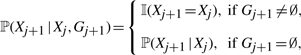
where the index j denotes the position along the sequence, and X_j∈ {1,…, k} and G_j ∈ {∅,1,…, k} are hidden states. The states X_j and G_j jointly determine the index c_j of the haplotype from which h_k+1,j (allele at the j-th site of h_k+1) is copied: if G_j = ∅ (the null state which indicates that the j-th site is not in a gene conversion tract), then c_j = X_j; otherwise, c_j = G_j. To capture the imperfect nature of the copying process resulting from mutation, the emission probability of the HMM is set up as follows:

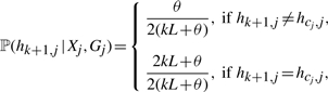(4)

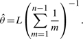
where L is the number of polymorphic sites in the input data (i.e. the length of each haplotype) and θ/L is the rate of mutation per site. If θ is not specified, it is estimated by using Watterson's unbiased estimator (Watterson, 1975):

(5)

Fig. 2.

Two different versions of HMM for computing the conditional probability . Unshaded circles represent hidden variables, whereas shaded ones correspond to observed variables. The symbols d_j denotes the physical distance between sites j and j + 1. In addition to a coupling of the two hidden chains, we allow pairwise overlaps of gene conversions. (a) A factorial HMM in which the two hidden chains are independent of each other. (Gay et al., 2007) used this model. (b) An interleaved HMM with coupled hidden chains.

As in the original PAC model of Li and Stephens (2003), crossover is modeled as a Poisson process with rate ρ across the sequence. The transition probability of the X chain has only two distinct cases, depending on whether the hidden states of adjacent sites are the same or not:

(6)

where d_j is the physical distance between sites j − 1 and j.

The transition probability of the G chain is more complicated. By assuming that the conversion tract length follows a geometric distribution, both initiation and termination of a conversion tract are modeled as Poisson processes along the sequence, with rates γ and 1/λ, respectively. Gay et al. used λ (not 1/λ) to denote the termination rate and assumed that the termination process goes on all the time, even when the copying process is not in a gene conversion state. Further, they make an additional assumption that conversion tracts from different gene conversion events cannot overlap. For example, consider the following probability of moving from state g ∈ {1,…, k} to state g′ ∈ {1,…, k}, where g ≠ g′:

(7)

This formulation requires terminating the gene conversion tract from g before initiating a new one from g′. The integrand corresponds to the probability of there being at least one gene conversion event after the last termination event at distance x to the left of site j + 1. In general, Gay et al.'s formulation implicitly allows for an infinite number of gene conversion initiation events to occur before the last termination event.

Lastly, the initial probability of the G chain depends on how the rate of starting a gene conversion tract compares to the rate of the ending one, i.e.

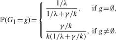In the above HMM formulation, it is straightforward to compute the conditional probability by using the standard forward–backward algorithm.

3 OUR MODEL

As described above, the work of Gay et al. (2007) assumes that crossovers and gene conversions are independent, and that gene conversion tracts cannot overlap. In this section, we construct a new model that couples the crossover and gene conversion processes. We then describe how overlapping gene conversions can be incorporated into the model.

3.1 Interleaved HMM

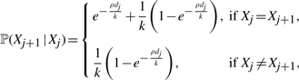
By assuming independence of the two hidden chains, the factorial HMM formulation of (Gay et al., 2007) cannot model the typical alternating pattern of gene conversion; i.e. a prefix of haplotype h followed by an internal fragment of a haplotype h′, which is then followed by a suffix of the first haplotype h. To remedy this, we couple the two hidden chains by using an interleaved HMM, illustrated in Figure 2b. Direct edges from the G chain to the X chain constrain the X chain to stay in its previous state whenever the G chain is ‘active’. More precisely,

(8)

where ℙ(X_j+1 ∣ X_j) in the second line is the same as in (6). If site j + 1 is in a conversion tract (i.e. G_j+1 ≠ ∅), the G chain is ‘active’ and the copying process keeps track of the previous state of the X chain (i.e. X_j+1 = X_j). If G_j+1 = ∅, the X chain evolves according to the usual transition probability ℙ(X_j+1 ∣ X_j).

We point out that coupling the two hidden chains does not increase the complexity of the forward–backward computation. Even in the factorial HMM, the two hidden chains become dependent upon conditioning on the observed variables. Therefore, the computational complexity is the same for both HMMs.

3.2 Modeling overlapping gene conversions

The key new feature of our model is that it allows for overlapping gene conversion events in the copying process. This means that the copying process does not need to terminate a gene conversion event before initiating another gene conversion event.

Figure 3 shows two examples of genealogies that can generate overlapping gene conversion tracts in the coalescent model with gene conversion (Wiuf and Hein, 2000). In Figure 3a, two gene conversion events have conversion tracts that overlap partially, while in Figure 3b, one conversion tract is entirely nested inside the other conversion tract.

Fig. 3.

Genealogical interpretations of overlapping gene conversions. Each genealogy contains two gene conversion events. Thin horizontal lines represent genetic material non-ancestral to the present-day sample, whereas thick horizontal lines correspond to ancestral material. Short vertical lines mark the boundaries of gene conversion tracts. (a) Two gene conversion tracts partially overlap. The left part of the blue conversion tract is non-ancestral because it is overwritten by the red conversion tract from a more recent gene conversion event. The ‘active’ haplotype in the region of overlapping gene conversion is g. (b) One conversion tract is completely nested inside the other conversion tract. The blue conversion tract overwrites the middle part of the red conversion tract. The ‘active’ haplotype in the region of overlap is g′.

Motivated by the common belief that the conversion tract length is typically short, between 50 bp and 2000 bp (Hilliker et al., 1994; Jeffreys and May, 2004), we restrict each overlap to involve only a pair of gene conversion events, although a generalization to more than two gene conversion events can easily be achieved at the expense of more computation time. In terms of the underlying HMM, we augment the state space of the G chain as follows. When computing , we include ordered pairs {(g, g′) ∣ g, g′ = 1,…, k} in the state space of the G chain, in addition to the singlet states {g∣g = ∅, 1,…, k} considered in Gay et al.'s model. If G_j = (g, g′), then site j of haplotype h_k+1 is within a region of overlapping gene conversion events involving two haplotypes h_g and h_g′. The second entry g′ in a doublet state (g, g′) is said to be ‘active’ and it indicates that the conversion tract from h_g′ overwrites the conversion tract from h_g at marker j of h_k+1. In Figure 3a, g is active in the region of overlapping gene conversions, while in Figure 3b g′ is active in the region of overlap. As in Gay et al.'s model, the hidden states X_j ∈ {1,…, k} and G_j jointly determine the index c_j of the haplotype from which h_k+1,j is copied. In our model,

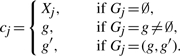We use the same emission probability as that shown in (4).

3.3 Transition probabilities for the augmented G chain

We now describe the transition probabilities ℙ(G_j+1 = s′ ∣ G_j = s) for the augmented G chain in the computation of . Instead of using the formulation described in (7), which implicitly allows for infinitely many gene conversion events between two adjacent sites, we explicitly enumerate all possible ‘valid’ paths of events defined to satisfy the following two properties: (i) each ‘valid’ path starts in state s and ends in state s′, and (ii) contains at most a initiations and b terminations of gene conversions. In our implementation, we use a = b = 1 for simplicity, but it is straightforward to consider larger values of a and b without increasing the asymptotic complexity of the forward–backward algorithm in our HMM.

For a = b = 1, the path (g, g′) → g′ → (g′, g″) is valid, since it contains exactly one initiation event and one termination event. In contrast, the path g → ∅ → g′ → (g, g′) is not valid since it contains two initiation events.

For a given pair of states s, s′ of the G chain (and for given values of a and b), all valid paths starting in s and ending in s′ can be enumerated using dynamic programming. We use 𝒫_s,s′ to denote the set of all such valid paths. To compute the probability ℙ(Γ) for a given path Γ ∈ 𝒫_s,s′, we make the following assumptions:

• Instead of allowing the termination process to run all the time, which Gay et al. (2007) assume, we assume that no termination event can occur if the current state in Γ is the ∅ state.

• If the current state in Γ is a singlet g, then an initiation event uniformly chooses g′ ∈ {1,…, k} and creates either (g, g′) or (g′, g) with equal probability; the termination process has rate 1/λ.

• If the current state in Γ is a doublet (g, g′), then no initiation can occur, since we assume only pairwise overlaps of gene conversions. The termination process has rate 2/λ, and when a termination event occurs, one makes a transition from (g, g′) to either g or g′ with equal probability.

With the above assumptions, ℙ(Γ) can be computed by integrating over all possible positions along the sequence where the events in Γ can happen. In contrast, recall that Gay et al. only integrate over the position of the last termination event. It turns out that the main computation involves a symbolic convolution of exponential functions, which can be easily evaluated. The transition probability ℙ(G_j+1 = s′ ∣ G_j = s) can be obtained by adding up the probability of all valid paths in 𝒫_s,s′ and then normalizing to make sure that the outgoing probabilities sum to 1, that is,

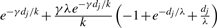
As a concrete example, consider the transition probability ℙ(G_j+1 = g′ ∣ G_{j = g}), where g, g′ ∈ {1,…, k} and g ≠ g′. For a = b = 1, 𝒫_g,g′ contains three valid paths, namely Γ₁ = g → ∅ → g′, Γ₂ = g → (g, g′) → g′ and Γ₃ = g → (g′, g) → g′. The probability of Γ₁ is given by

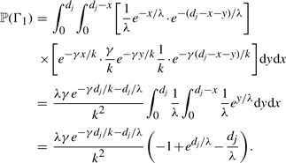The integrand corresponds to the probability of there being exactly one termination event and exactly one initiation event, with the termination (respectively, initiation) event occurring at distance x (respectively, x + y) to the right of site j. Integrating over all possible values of x and y yields the probability of Γ₁. In a similar vein, one can show that the probabilities ℙ(Γ₂) and ℙ(Γ₃) are given by

The transition probability ℙ(G_j+1 = g′ ∣ G_j = g) is proportional to ℙ(Γ₁)+ℙ(Γ₂)+ℙ(Γ₃).

Table 1 lists the transition probabilities in the G chain of our implementation with a = b = 1. In the table, g, g′ and g″ denote distinct elements of {1,…, k}.

Table 1.

Transition probabilities ℙ(G_j+1=s′ ∣ G_{j = s}) for the gene conversion chain in the computation of , assuming at most one initiation and at most one termination of gene conversions between adjacent sites

State s at marker j	State s′ at marker j + 1	ℙ(Gj+1 = s′∣Gj = s) up to normalization
∅	∅
∅	g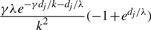
g	(g, g)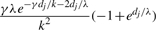
g	(g, g′)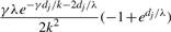
g	g
g	g′
g	∅	e−γdj/k(1 − e−dj/λ)
(g, g)	(g, g)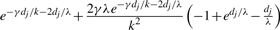
(g, g)	(g, g′)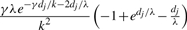
(g, g)	g	2e−γdj/k−dj/λ(1 − e−dj/λ)
(g, g′)	(g, g) or (g′, g′) or (g′, g)
(g, g′)	(g, g′)
(g, g′)	(g, g″) or (g′, g″)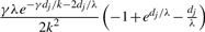
(g, g′)	g or g′	e−γdj/k−dj/λ(1−e−dj/λ)

Here, g, g′ and g″ denote distinct elements of {1,…, k}.

3.4 Initial probabilities of the G chain

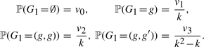
We wish to use the stationary distribution of the transition matrix of the G chain as the initial probability at the first SNP site. However, in the computation of , the size of the transition matrix is (1 + k + k²) × (1 + k + k²), since there are 1 null state ∅, k singlet states (g), k degenerate doublet states (g, g) and k² − k non-degenerate doublet states (g, g′), where g ≠ g′. Finding an eigenvector of that transition matrix could be computationally expensive for moderate values of k. Therefore, we make the following approximation: we collapse the transition matrix to a 4 × 4 matrix, whose rows and columns are indexed by ‘null’, ‘singlet’, ‘degenerate doublet’ and ‘non-degenerate doublet’. Each entry in the collapsed matrix is obtained by summing over the corresponding entries in the original transition matrix. We find the left eigenvector v = (v₀, v₁, v₂, v₃) of the collapsed matrix with eigenvalue 1. Then, for g, g′ ∈ {1,…, k}, where g ≠ g′, the initial probabilities of the G chain are specified as

3.5 Complexity of the algorithm

Since the augmented HMM has O(k³) states when computing , a naive implementation of the forward–backward algorithm takes O(k⁶L) time, where L is the number of polymorphic sites in the input data (i.e. the length of each haplotype). Hence, the computational complexity of the PAC likelihood L_PAC (for fixed parameters ρ, γ, λ) in our model is O(n⁷L), where n is the total number of input haplotypes. However, by exploiting the sparsity and regularity of transition probabilities, we can use algorithmic shortcuts to reduce the complexity to O(n⁴L). As in Gay et al.'s method, we use a standard derivative-free optimization procedure to find the maximum likelihood estimates of ρ, γ and λ based on L_PAC.

4 RESULTS

In this section, we summarize the performance of our method on simulated data and then consider a real biological application. In both cases, we compare our method with GenCo, the method developed by Gay et al. (2007).

4.1 Simulation study

To test the performance of our method, we used Hudson's (2002) coalescent simulation program MS to generate simulated datasets. In general, it is possible that the evolutionary history of a particular region R in a genome involves gene conversions with one end of the conversion tract falling outside R and the other end falling within R. To account for such events, we simulated a 30 kb region and then discarded 5 kb from each end. In all simulations, we used θ = 1.0/kb for mutation rate and λ=0.5 kb for the mean conversion tract length, both of which being relevant to humans [see Ptak et al. (2004) and Frisse et al. (2001), respectively]. For each dataset, both GenCo and our method were each run 10 times, taking 20 random permutations of haplotype order in each iteration. The same permutations were used in the two methods. In the first iteration, both GenCo and our method started the optimization procedure at the true values of ρ,γ and λ, while in the subsequent iterations, the maximum likelihood estimates from the previous iteration were used as initial values. For the crossover rate, we used ρ = 0.5 or 1.0/kb, while for the gene conversion rate, we used γ = 0.5, 1.0 or 2.5/kb. For each parameter setting, we generated 100 simulated datasets each with 20 haplotypes. For each simulated dataset, we estimated all three parameters ρ, γ and λ, while θ was set to Watterson's estimate (5). Shown in Table 2 is a summary of performance results. The columns labeled and display the mean and SD (shown in parentheses) of the corresponding estimates. The column labeled shows the number of datasets with crossover estimates within a factor of k from the true ρ; and the columns labeled and are similarly defined for gene conversion rate γ and the mean tract length λ, respectively.

Table 2.

Comparison of our method with GenCo on simulated data

ρ	γ	λ	Method
0.5	0.5	0.5	GenCo	0.51 (0.43)	3700 (23000)	1.4 (9.0)	66	29	26	98	64	62
			Ours	0.48 (0.27)	1.7 (1.6)	0.50 (0.29)	75	37	83	99	96	100
0.5	1.0	0.5	GenCo	0.48 (0.47)	670 (4000)	0.56 (0.79)	76	47	45	98	79	78
			Ours	0.46 (0.23)	2.0 (1.7)	0.49 (0.29)	78	59	80	99	98	100
0.5	2.5	0.5	GenCo	0.59 (0.62)	66 (560)	1.1 (4.1)	81	78	75	98	96	94
			Ours	0.59 (0.27)	2.3 (1.2)	0.45 (0.15)	83	83	93	100	100	100
1.0	0.5	0.5	GenCo	0.84 (0.43)	380 (1200)	1.1 (3.5)	78	17	27	98	61	57
			Ours	0.79 (0.26)	1.8 (2.6)	0.51 (0.30)	84	31	82	99	96	98
1.0	1.0	0.5	GenCo	0.79 (0.40)	230 (820)	0.91 (2.01)	77	55	49	99	79	76
			Ours	0.81 (0.35)	1.8 (1.5)	0.51 (0.25)	86	71	85	100	99	100
1.0	2.5	0.5	GenCo	0.93 (1.30)	370 (2100)	1.3 (6.4)	71	71	60	98	88	85
			Ours	0.85 (0.35)	2.6 (1.5)	0.44 (0.18)	80	86	85	100	100	100

The estimates of ρ and γ are per kilobase. For each triplet (ρ, γ, λ), we generated 100 simulated datasets using MS (Hudson, 2002) for θ = 1.0/kb and 20 haplotypes. Shown in the columns labeled , and are the mean and SD (shown in parentheses) of the corresponding parameter estimates. The symbol denotes the number of data sets with an estimate within a factor of k from the true ρ. The symbols and are similarly defined for γ and λ, respectively.

4.1.1 Estimation of ρ

Both our method and GenCo produced reasonable estimates of ρ. The two estimates had similar means, but our estimate generally had a smaller variance than that of GenCo.

4.1.2 Estimation of γ

Our improvement over GenCo is clearly illustrated in the estimation of γ. GenCo's estimate of γ was substantially biased upward, with means above the true γ by factors of tens to thousands. In most cases, this significant bias was not a result of only a few outliers; as the column labeled in Table 2 and the histogram in Figure 4a show, GenCo produced very large estimates of γ for a significant fraction of simulated datasets. In contrast, as Table 2 and the histogram in Figure 4b indicate, our estimate of γ was much more well behaved for all parameter settings, though it was slightly biased upward for γ = 0.5 and 1.0/kb.

Fig. 4.

Histogram of gene conversion rate estimates and mean conversion tract length estimates relative to their true values. Based on 100 simulations with n = 20, ρ = γ = 1.0/kb and λ = 0.5 kb.

4.1.3 Estimation of λ

GenCo's estimate of λ was slighted biased upward. This upward bias occurred even though many estimates were well below the true value λ = 0.5 kb, as shown in the histogram in Figure 4c. In GenCo, a very large was usually accompanied by a very small . In comparison, as Table 2 and the histogram in Figure 4d show, our estimate of λ is much more accurate, with a smaller variance. However, as the cases with γ = 2.5/kb suggest, our estimate of the mean tract length λ seems slightly biased downward when γ is large.

4.2 A real biological application

Gay et al. (2007) used their method to study recombination patterns in two genes—namely, su(s) and su(w^a) surveyed by Langley et al. (2000)—located near the telomere of the X chromosome of D.melanogaster. The su(s) and su(w^a) loci are about 4.1 kb and 2.5 kb long, respectively, and are about 400 kb apart. Langley et al. (2000) surveyed samples from both an African and an European population, but only the African sample was considered by Gay et al., and we do the same here. The su(s) dataset contains 50 haplotypes and 41 SNPs, while the su(w^a) dataset contains 50 haplotypes and 46 SNPs.

Gay et al. reported that, upon fixing the mean tract length to 0.352 kb (Hilliker et al., 1994), they obtained and , thus concluding . In their paper, Gay et al. did not specify whether the above estimates were for the su(s) locus or the su(w^a) locus. To compare their method GenCo with our method, we redid the analysis, following the same procedure as in Section 4.1, i.e. taking 20 random permutations of haplotype order and iterating the computation 10 times. We used ρ = 1.0/kb and γ = 1.0/kb as the starting values of the optimization procedure in the first iteration. The results, summarized in Table 3, are quite different between the two methods. Assuming λ = 0.352 kb, GenCo suggests that the gene conversion rate is substantially higher than the crossover rate in each gene, while our method implies that the two rates are comparable.

Table 3.

Estimates of ρ and γ for the su(s) and su(w^a) loci in D.melanogaster, with λ held fixed at 0.352 kb

Gene	Method
su(s)	GenCo	1.7	12	7.1
	Ours	3.9	5.1	1.3
su(wa)	GenCo	0.57	28	48
	Ours	9.4	7.1	0.76

The estimates of ρ and γ are per kilobase.

We also performed analysis with λ as a free parameter; Gay et al. (2007) did not consider this analysis in their paper. In this case, we used ρ = 5.0/kb, γ = 5.0/kb, and λ = 0.352 kb as the starting values of the optimization procedure in the first iteration. GenCo and our method again produced generally different results. The corresponding maximum likelihood estimates of ρ, γ and λ are shown in Table 4. For the su(s) locus, GenCo and our method produced similar estimates of γ, but GenCo produced a much smaller estimate of ρ than that of our method, while the opposite is true for . For the su(w^a) locus, GenCo and our method produced similar estimates of ρ, but GenCo produced a much larger estimate of γ than that of our method, though both methods produced a value of that was substantially larger than . The estimates of λ in both methods were quite small; this could be an artifact of the methods, which tend to produce small estimates of λ when estimates of γ are large.

Table 4.

Estimates of ρ, γ and λ for the su(s) and su(w^a) loci in D.melanogaster

Gene	Method
su(s)	GenCo	0.78	10	13	0.55
	Ours	4.7	11	2	0.13
su(wa)	GenCo	9.9	270	27	0.004
	Ours	9.4	96	10	0.015

The estimates of ρ and γ are per kilobase, while the estimate of λ is in kilobase.

As discussed in Section 4.1, both GenCo and our method tend to overestimate γ (GenCo more so than our method), but the fact that both methods detected strong signals of gene conversion suggests that gene conversion is likely to have played an important role in shaping the observed pattern of genetic variation in the two genes. This agrees with Langley et al.'s conclusion. However, unlike what Gay et al. (2007) concluded, our analysis implies that crossover may not have been greatly suppressed in the su(s) and su(w^a) loci.

5 DISCUSSION

High-throughput sequencing technology has advanced remarkably in the past few years (Bentley, 2006), and soon it will become routine to obtain whole-genome sequence information. Such fine-scale data from populations will allow us to quantify fundamental population genetics parameters with high accuracy. In particular, it will soon be possible to provide a genomic annotation of gene conversion rates and characterize the distribution of conversion tract lengths. Hence, improved algorithms and statistical tools for studying gene conversion are much in need.

In this article, we have developed a model that allows overlapping gene conversions. We believe that this aspect of our model is crucial in making the joint estimation of the gene conversion rate and the mean conversion tract length feasible. Although the joint estimation of the three parameters ρ,γ and λ is indeed a very difficult problem, and the method proposed here is unlikely to be optimal, we believe that we have taken an important step towards devising a robust, reliable method.

Our current method can be improved in several ways. When the gene conversion rate γ is high, our method tends to underestimate the conversion tract length λ slightly. On the other hand, when γ is small, our method tends to overestimate γ slightly. We believe that both biases can be corrected by considering larger threshold values (a and b) on the maximum number of allowed gene conversion initiation and termination events. We will explore this improvement in the future. Other important future directions include handling missing data and variable rates across the sequence.

The PAC model proposed by Li and Stephens (2003) is a useful framework with many applications. Hellenthal et al. (2008) recently proposed using a PAC-based copying model to infer human colonization history. Clearly, the accuracy of that inference method can benefit from having a more realistic copying model, as that proposed here.

REFERENCES

- Bentley DR. Whole-genome re-sequencing. Curr. Opin. Genet. Dev. 2006;16:545–552. doi: 10.1016/j.gde.2006.10.009. [DOI] [PubMed] [Google Scholar]
- Crawford DC, et al. Evidence for substantial fine-scale variation in recombination rates across the human genome. Nat. Genet. 2004;36:700–706. doi: 10.1038/ng1376. [DOI] [PubMed] [Google Scholar]
- Frisse L, et al. Gene conversion and different population histories may explain the contrast between polymorphism and linkage disequilibrium levels. Am. J. Hum. Genet. 2001;69:831–843. doi: 10.1086/323612. [DOI] [PMC free article] [PubMed] [Google Scholar]
- Gay JC, et al. Estimating meiotic gene conversion rates from population genetic data. Genetics. 2007;177:881–894. doi: 10.1534/genetics.107.078907. [DOI] [PMC free article] [PubMed] [Google Scholar]
- Ghahramani Z, Jordan MI. Factorial hidden Markov models. Mach. Learn. 1997;29:245–273. [Google Scholar]
- Hellenthal G. PhD Thesis. Seattle: University of Washington; 2006. Exploring Rates and Patterns of Variability in Gene Conversion and Crossover in the Human Genome. [Google Scholar]
- Hellenthal G, et al. Inferring human colonization history using a copying model. PLoS Genet. 2008;4:e1000078. doi: 10.1371/journal.pgen.1000078. [DOI] [PMC free article] [PubMed] [Google Scholar]
- Hilliker AJ, et al. Meiotic gene conversion tract length distribution within the rosy locus of Drosophila melanogaster. Genetics. 1994;137:1019–1026. doi: 10.1093/genetics/137.4.1019. [DOI] [PMC free article] [PubMed] [Google Scholar]
- Hudson RR. Properties of a neutral allele model with intragenic recombination. Theor. Popul. Biol. 1983;23:183–201. doi: 10.1016/0040-5809(83)90013-8. [DOI] [PubMed] [Google Scholar]
- Hudson RR. Two-locus sampling distributions and their application. Genetics. 2001;159:1805–1817. doi: 10.1093/genetics/159.4.1805. [DOI] [PMC free article] [PubMed] [Google Scholar]
- Hudson RR. Generating samples under the Wright-Fisher neutral model of genetic variation. Bioinformatics. 2002;18:337–338. doi: 10.1093/bioinformatics/18.2.337. [DOI] [PubMed] [Google Scholar]
- Hwang DG, Green P. Bayesian Markov chain Monte Carlo sequence analysis reveals varying neutral substitution patterns in mammalian evolution. Proc. Natl Acad. Sci. USA. 2004;101:13994–14001. doi: 10.1073/pnas.0404142101. [DOI] [PMC free article] [PubMed] [Google Scholar]
- International HapMap Consortium. A haplotype map of the human genome. Nature. 2005;437:1299–1320. doi: 10.1038/nature04226. [DOI] [PMC free article] [PubMed] [Google Scholar]
- Jeffreys AJ, May CA. Intense and highly localized gene conversion activity in human meiotic crossover hot spots. Nat. Genet. 2004;36:151–156. doi: 10.1038/ng1287. [DOI] [PubMed] [Google Scholar]
- Kingman JFC. The coalescent. Stoch. Process. Appl. 1982;13:235–248. [Google Scholar]
- Langley CH, et al. Linkage disequilibria and the site frequency spectra in the su(s) and su(wa) regions of the Drosophila melanogaster X chromosome. Genetics. 2000;156:1837–1852. doi: 10.1093/genetics/156.4.1837. [DOI] [PMC free article] [PubMed] [Google Scholar]
- Li N, Stephens M. Modeling linkage disequilibrium and identifying recombination hotspots using single-nucleotide polymorphism data. Genetics. 2003;165:2213–2233. doi: 10.1093/genetics/165.4.2213. [DOI] [PMC free article] [PubMed] [Google Scholar]
- Mancera E, et al. High-resolution mapping of meiotic crossovers and non-crossovers in yeast. Nature. 2008;454:479–485. doi: 10.1038/nature07135. [DOI] [PMC free article] [PubMed] [Google Scholar]
- Myers S, et al. A fine-scale map of recombination rates and hotspots across the human genome. Science. 2005;310:321–324. doi: 10.1126/science.1117196. [DOI] [PubMed] [Google Scholar]
- Padhukasahasram B, et al. Estimating recombination rates from single-nucleotide polymorphisms using summary statistics. Genetics. 2006;174:1517–1528. doi: 10.1534/genetics.106.060723. [DOI] [PMC free article] [PubMed] [Google Scholar]
- Pritchard JK, Przeworski M. Linkage disequilibrium in humans: models and data. Am. J. Hum. Genet. 2001;69:1–14. doi: 10.1086/321275. [DOI] [PMC free article] [PubMed] [Google Scholar]
- Ptak SE, et al. Insights into recombination from patterns of linkage disequilibrium in humans. Genetics. 2004;167:387–397. doi: 10.1534/genetics.167.1.387. [DOI] [PMC free article] [PubMed] [Google Scholar]
- Rabiner L. A tutorial on HMM and selected applications in speech recognition. Proc. IEEE. 1989;77:257–286. [Google Scholar]
- Song YS, et al. Algorithms to distinguish the role of gene-conversion from single-crossover recombination in the derivation of SNP sequences in populations. J. Comput. Biol. 2007;14:1273–1286. doi: 10.1089/cmb.2007.0096. [DOI] [PMC free article] [PubMed] [Google Scholar]
- Voight BF, et al. A map of recent positive selection in the human genome. PLoS Biol. 2006;4:e72. doi: 10.1371/journal.pbio.0040072. [DOI] [PMC free article] [PubMed] [Google Scholar]
- Wall JD. Close look at gene conversion hot spots. Nat. Genet. 2004a;36:114–115. doi: 10.1038/ng0204-114. [DOI] [PubMed] [Google Scholar]
- Wall JD. Estimating recombination rates using three-site likelihoods. Genetics. 2004b;167:1461–1473. doi: 10.1534/genetics.103.025742. [DOI] [PMC free article] [PubMed] [Google Scholar]
- Watterson G. On the number of segregation sites. Theor. Popul. Biol. 1975;7:256–276. doi: 10.1016/0040-5809(75)90020-9. [DOI] [PubMed] [Google Scholar]
- Wiuf C, Hein J. The coalescent with gene conversion. Genetics. 2000;155:451–462. doi: 10.1093/genetics/155.1.451. [DOI] [PMC free article] [PubMed] [Google Scholar]