Bioinformatics Methods for Learning Radiation-Induced Lung Inflammation from Heterogeneous Retrospective and Prospective Data

Abstract

Radiotherapy outcomes are determined by complex interactions between physical and biological factors, reflecting both treatment conditions and underlying genetics. Recent advances in radiotherapy and biotechnology provide new opportunities and challenges for predicting radiation-induced toxicities, particularly radiation pneumonitis (RP), in lung cancer patients. In this work, we utilize datamining methods based on machine learning to build a predictive model of lung injury by retrospective analysis of treatment planning archives. In addition, biomarkers for this model are extracted from a prospective clinical trial that collects blood serum samples at multiple time points. We utilize a 3-way proteomics methodology to screen for differentially expressed proteins that are related to RP. Our preliminary results demonstrate that kernel methods can capture nonlinear dose-volume interactions, but fail to address missing biological factors. Our proteomics strategy yielded promising protein candidates, but their role in RP as well as their interactions with dose-volume metrics remain to be determined.

1. Introduction

Lung cancer is one of the most lethal diseases among men and women worldwide. Patients suffering from lung cancer display a 5-year survival rate of only 15%, a value that has held constant over the past 30 years. According to the American Cancer Society (ACS) statistics, 215.020 new lung cancer cases and 161.840 deaths due to lung cancer are expected in the year 2008 alone [1]. This accounts for 29% of all cancer deaths with 87% of these cases classified clinically as nonsmall cell lung cancer (NSCLC). A large percentage of lung cancer patients receive radiation therapy (radiotherapy) as part of their standard of care and it is the main treatment for inoperable patients at advanced stages of the disease. Radiotherapy is a directed and localized treatment, but its dose is limited by toxicities to surrounding normal tissues. Thus, patients are at risk of experiencing tumor recurrence if insufficient dose was prescribed or conversely they are susceptible to toxicities if exposed to excessive doses.

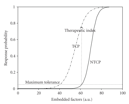
The last two decades have witnessed many technological advances in the development of three-dimensional treatment planning systems and image-guided methods to improve tumor localization while sparing surrounding normal tissues [2, 3]. In parallel, there has been a tremendous evolution in biotechnology providing high-throughput genomics and proteomics information applicable within cancer radiation biology. This has led to the birth of a new field in radiation oncology denoted as “radiogenomics” or “radioproteomics” [4, 5]. These advances, if directed properly, could pave the way for increasingly individualized and patient-specific treatment planning decisions that continue to draw from estimates of tumor local control probability (TCP) or surrounding normal tissues complication probability (NTCP) as illustrated in Figure 1.

Figure 1.

An S-shaped response curves representing tumor control probability (TCP) and normal tissue complication probability (NTCP) postradiotherapy as a function of treatment factors. The probabilities could be constructed as a function of heterogeneous variables (dose-volume metrics, biomarkers, and clinical factors). The radiotherapy treatment objective is to maximize the therapeutic index for each patient case.

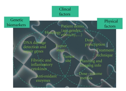
Traditionally, tissue radioresponse has been modeled using simplistic expressions of cell kill based on the linear-quadratic (LQ) model developed in the 1940s [6]. The LQ formalism describes repairable and nonrepairable radiation damage of different tissue types with a few estimated radiation sensitivity parameters from cell culture assays [7]. Despite the historical value of LQ-based models, several authors have recently cautioned against its limitations [8, 9]. It is understood that radiotherapy outcomes are determined by complex interactions between physical treatment factors, anatomical structures, and patient-related genetic variables as depicted in Figure 2.

Figure 2.

Radiotherapy treatment involves complex interaction of physical, biological, and clinical factors. The successful datamining approach should be able to resolve this interaction “puzzle” in the observed treatment outcome (e.g., radiation-induced lung injury) for each individual patient.

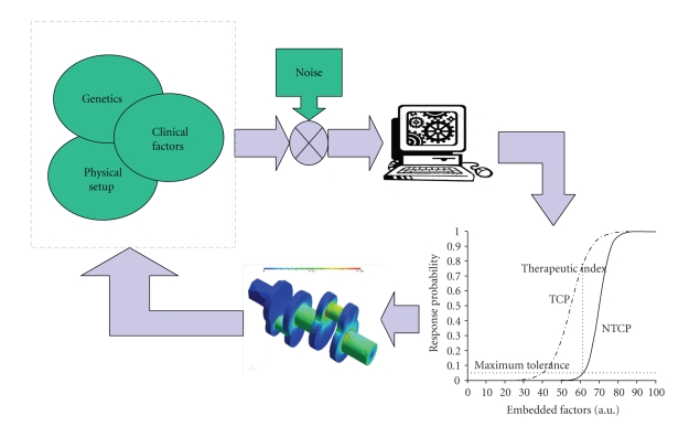
A different approach based on datamining of patient information (clinical, physical, and biological records) has been proposed to ameliorate these challenges and bridge the gap between traditional radiobiological predictions from in vitro assays and observed treatment outcomes in clinical practice by understanding the underlying molecular mechanisms [10–12]. The main idea of data-driven models is to utilize datamining approaches and statistical model building methods to integrate disparate predictive factors. Such models may improve predictive power, but they must be simultaneously guarded for overfitting pitfalls using resampling techniques, for instance. This approach is motivated by the extraordinary increase in patient-specific biological and clinical information from progress in genetics and imaging technology. The main goal is to resolve the complicated interactions by proper mixing of heterogeneous variables (Figure 2). As a result, the treatment planning system could be optimized to yield the best possible care for the patient as illustrated in Figure 3.

Figure 3.

The datamining understanding of these heterogeneous variables interactions could be fed back into the treatment planning system to improve patient's outcomes.

Most data-driven models in the radiation oncology literature could be categorized into two types of models: (1) physical dose-volume models or (2) single-biomarkers models. Dose-volume models are driven by the presence of large treatment planning archives and the current clinical practice of radiotherapy treatment. Current radiotherapy protocols allow for the extraction of parameters that relate irradiation dose to the treated volume fractions (tumors or surrounding normal organs at risk) in dose-volume histograms [13]. Conversely, screening for different blood/tissue biomarkers to predict radiation response (TCP or NTCP) is an emerging field in radiation oncology with many promising opportunities as well as new technical challenges regarding data collection quality, the advancement of lab techniques, and the development of statistical methodology [14].

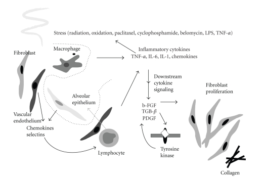
To illustrate and investigate the changing landscape of radiation response modeling, our study addresses radiation pneumonitis (RP), the major dose limiting toxicity in thoracic irradiation. Clinically, RP is lung inflammation that usually occurs within six months after therapy for a subset of patients and can manifest as cough, dyspnea, fever, and/or malaise which may require significant supportive measures including steroids and oxygen supplementation [15]. In its worst form, RP can continue to progress and result in death. According to the NCI Common Terminology Criteria for Adverse Events (CTCAEs) v3.0, a clinical scoring system for RP, the severity of pneumonitis is graded from 0 (minimal symptoms) to 4 (most severe/life-threatening) or even 5 (death). A CTCAE-v3.0 grade ≥3 indicates clinical onset of severe RP. Biologically, the ionizing radiation from treatment can cause damage to the normal alveolar epithelium cells (airways) of the lung resulting in release of a wetting agent surfactant into the alveolar space and detachment of the pneumocytes from their basement membrane. It is thought that this process triggers a cascade of humoral cellular and immune response events among alveolar epithelium, fibroblasts, lymphocytes, and macrophages leading to RP as shown in Figure 4 [16].

Figure 4.

A schematic diagram of the possible cellular and molecular events involved in pulmonary injury by radiation. Cellular interaction among endothelial cells, alveolar epithelial cells, macrophages, lymphocytes, and fibroblasts, through cytokine mediators of chemokines, selectins, inflammatory cytokines, and fibrotic cytokines are involved (from Chen et al., Seminars in Surgical Oncology, 2003).

We conjecture that a good predictive model for radiation hypersensitivity should be able to properly describe the interactions between physical and biological processes resulting from radiation exposure and adequately span the variable space shown in Figure 2. Working towards this standard, we will present our utilization of supervised and unsupervised machine learning approaches to interrogate radiation oncology data and develop methodology for building better predictive models of radiation therapy response. We start by examining existing treatment planning archives and conduct retrospective analysis of physical dose-volume models to predict the onset of RP. We then describe our attempt to fillin the prediction gap in such physical models through a prospective study that considers preexisting biological variables, which may influence treatment response. Note that the retrospective study has the advantage of large sample size and hence higher power while the prospective approach is focused towards improving current prediction by incorporating missing information in past archives into more comprehensive databases and performing evaluation on new unseen data. In particular, we will present our proteomic methodology to investigate predictive biomarkers of RP that could eliminate informational gaps in our retrospective physical model.

The paper is organized as follows. In Section 2, we describe our retrospective analysis of dose-volume RP predictors and our current prospective proteomic analysis. In Section 3, we contrast our results using model-building approaches based on logistic regression, support vector machine, and a 3-way design for biomarker discovery in proteomic analysis of RP. Methods for variable selections are analyzed. Lastly, in Section 4 we discuss our current findings and offer some concluding remarks in Section 5.

2. Materials and Methods

2.1. Dataset Description

To demonstrate our methodology, separate datasets were compiled using data from two groups of patients all diagnosed with nonsmall cell lung cancer (NSCLC) and treated with three-dimensional conformal radiation therapy (3D-CRT) at our institution. The first dataset was collected retrospectively from the clinical archives with median doses around 70 Gy (the doses were corrected to account for lung heterogeneity using the tissue-air ratio method). In this set, 52 out of 219 patients were diagnosed with postradiation late pneumonitis (RTOG grade ≥3). The dataset included clinical and dosimetric (dose-volume) variables. The clinical variables included age, gender, ethnicity, date of treatment start, treatment technique, treatment aim, chemotherapy, disease stage, treatment duration, histological features, and so forth. The dosimetric variables compiled for this retrospective dataset were measured and calculated in reference to the extensive dose-volume documentation in the radiation oncology literature. Typically, these metrics are extracted from the dose-volume histogram (DVH) and include V_x (the percentage volume that got x Gy), D_x (the minimum dose to the hottest x% volume), mean dose, maximum and minimum doses, generalized equivalent uniform, and so forth. In-house software tools for data dearchiving, the analysis software a Computational Environment for Radiotherapy Research (CERR) [17], and the dose response explorer system (DREES) [18] were used to extract the different metrics and analyze their association with RP.

The second dataset was collected from September 2007 to September 2008 for a prospective analysis. Nineteen patients were involved in the study and underwent conventional radiotherapy with mean doses close to 70 Gy. Out of nineteen patients, four were diagnosed with postradiation late pneumonitis (RTOG grade ≥3). The data collected for each patient included the same clinical and dosimetric variables as the prospective study. In addition to this data, five blood samples were drawn from each patient over the course of treatment. These sample collections were scheduled before radiotherapy (pretreatment), midtreatment, immediately after radiotherapy (posttreatment), and also at a three month and at six-month follow-up appointments.

This second dataset is gathered from an institutionally approved prospective study for extracting biomarkers to predict radiotherapy response in inoperable stage III NSCLC patients who receive radiotherapy as part of their treatment. For our preliminary proteomic screening, we selected two lung cancer patients who were treated using fractionated radiotherapy according to our institute clinical standards. One case was designated as control and the other case was for a patient who developed RP and designated as disease. The control patient, despite radiation treatment for advanced lung cancer, developed no adverse health conditions throughout a follow-up period of 14 months. RP typically occurs within the first year posttreatment with a mode of 6 months. The disease case selected for the study died due to a severe RP episode one month after the end of treatment. For both the control and disease cases, a serum sample drawn before treatment as well as a sample drawn at the last available follow-up was submitted for liquid chromatography mass spectrometry (LC-MS) analysis. A Seppro 15 × 13 mm chromatography column (LC20) (GenWay Biotech Inc., San Diego, Calif, USA) was used to deplete the thawed samples of the 14 most abundant proteins in human blood serum. The samples then underwent digestion by the serine protease trypsin with a 10 μg Bovine Serum Albumin (BSA) external standard. Subsequent LC-MS allowed for the separation and mass analysis of tryptic peptides in each of the four samples. The most abundant peptides of each MS mass scan were automatically sent to a second mass spectrometer for fragmentation and sequence determination according to a tandem MS (MS/MS) design.

2.2. Model Building Approach

In the context of data-driven outcomes modeling, the observed treatment outcome (e.g., normal tissue complication probability (NTCP) or tumor control probability (TCP) is considered as the result of functional mapping of multiple dosimetric, clinical, or biological input variables [19]. Mathematically, this could be expressed as f(x;w*) : X → Y, where x_i ∈ ℝ^d are the input explanatory variables (dose-volume metrics, patient disease specific prognostic factors, or biological markers) of length d, y_i ∈ Y are the corresponding observed treatment outcome (TCP or NTCP), and w* includes the optimal parameters of outcome model f(·) obtained by optimizing a certain objective criteria. In our previous work [10, 19], a logit transformation was used as follows:

$$f\left({\mathbf{x}}_i\right)=\frac{e^{g\left({\mathbf{x}}_i\right)}}{1+e^{g\left({\mathbf{x}}_i\right)}},\hspace{1em}i=1,\dots ,n,$$ (1)

where n is the number of cases (patients), x_i is a vector of the input variable values used to predict f(x_i) for outcome y_i of the ith patient. The “x-axis” summation g(x_i) is given by

$$g\left({\mathbf{x}}_i\right)={\beta }_o+{\displaystyle \sum }_{j=1}^d\hspace{0.17em}{\beta }_j{x}_{ij},\hspace{1em}i=1,\dots ,n,j=1,\dots ,d,$$ (2)

where d is the number of model variables and the β's are the set of model coefficients determined by maximizing the probability that the data gave rise to the observations. A major weakness in using this formulation, however, is that the model capacity to learn is limited. In addition, (2) requires the user feedback to determine whether interaction terms or higher order terms should be added, making it a trial and error process. A solution to ameliorate this problem is offered by applying machine learning methods as discussed in the next section.

2.3. Kernel-Based Methods

Kernel-based methods and their most prominent member, support vector machines (SVMs), are universal constructive learning procedures based on the statistical learning theory [20]. These methods have been applied successfully in many diverse areas [21–25].

Statistical Learning —

Learning is defined in this context as estimating dependencies from data [26]. There are two common types of learning: supervised and unsupervised. Supervised learning is used to estimate an unknown (input, output) mapping from known (input, output) samples (e.g., classification or regression). In unsupervised learning, only input samples are given to the learning system (e.g., clustering or dimensionality reduction). In this study, we focus mainly on supervised learning, wherein the endpoints of the treatments such as tumor control or toxicity grade are provided by experienced oncologists following RTOG or NCI criteria. Nevertheless, we will use unsupervised methods such as principle component analysis and multidimensional scaling to aid visualization of multivariate data and guide the selection of proper schemes for data analysis.

The main objective of supervised learning is to estimate a parametric function f(x;w*) : X → Y by assistance from a representative training set {(x_i, y_i)}_{i = 1}ⁿ. The two main supervised learning tasks are classification and regression. The difference between classification and regression is that the output y in case of classification belongs to a discrete, or categorical, set y ∈ {1, 2,…, M} (e.g., in binary classification M = 2), whereas in regression y is a continuous variable. In the example of classification (i.e., discrimination between patients who are at low risk versus patients who are at high risk of radiation pneumonitis), the main function of the kernel-based technique would be to separate these two classes with “hyperplanes” that maximize the margin (separation) between the classes in the nonlinear feature space defined by implicit kernel mapping. The objective here is to minimize the bounds on the generalization error of a model on unseen data before rather than minimizing the mean-square error over the training dataset itself (data fitting). Consequently, the optimization problem could be formulated as minimizing the following cost function:

$$L\left(\mathbf{w},\xi \right)=\frac{1}{2}{\mathbf{w}}^T\mathbf{w}+C{\displaystyle \sum }_{i=1}^n{\xi }_i,$$ (3)

subject to the constraint:

$$\begin{array}{c}{y}_i\left({\mathbf{w}}^T\Phi \left({\mathbf{x}}_i\right)+b\right)\ge 1-{\zeta }_i,\hspace{1em}i=\mathrm{1,2},\dots ,n,\\ {\zeta }_i\ge 0\hspace{1em}\forall i,\end{array}$$ (4)

where w is a weighting vector and Φ(·) is a nonlinear mapping function. The ζ_i represents the tolerance error allowed for each sample to be on the wrong side of the margin (called hinge loss). Note that minimization of the first term in (3) increases the separation (margin) between the two classes, whereas minimization of the second term improves fitting accuracy. The tradeoff between complexity (or margin separation) and fitting error is controlled by the regularization parameter C.

It stands to reason that such a nonlinear formulation would suffer from the curse of dimensionality (i.e., the dimensions of the problem become too large to solve) [26, 27]. However, computational efficiency is achieved from solving the dual optimization problem instead of (3). The dual optimization problem is convex but positive-semidefinite (global but not necessarily unique solution). However, the complexity in this case is dependent only on the number of samples and not on the dimensionality of the feature space. Moreover, because of its rigorous mathematical foundations, it overcomes the “black box” stigma of other learning methods such as neural networks. The prediction function in this case is characterized by only a subset of the training data known as support vectors s_i:

$$f\left(\mathbf{x}\right)={\displaystyle \sum }_{i=1}^{n_s}{\alpha }_i{y}_{i}K\left({\mathbf{s}}_i,\mathbf{x}\right)+{\alpha }_0,$$ (5)

where n_s is the number of support vectors, α_i are the dual coefficients determined by quadratic programming, and K(·, ·) is the kernel function. Typical kernels include

$$\begin{array}{ll}& \text{Polynomials:}\hspace{0.17em}K(\mathbf{x},{\mathbf{x}}^{\prime })={({\mathbf{x}}^T{\mathbf{x}}^{\prime }+c)}^q\\ & \text{Radial}\hspace{0.17em}\text{basis}\hspace{0.17em}\text{function}\hspace{0.17em}\left(\text{RBF}\right)\text{:}\hspace{0.17em}\hspace{0.17em}K\left(\mathbf{x},{\mathbf{x}}^{\prime }\right)=\text{exp}\hspace{0.17em}(-\frac{1}{2{\sigma }^2}{\parallel \mathbf{x}-{\mathbf{x}}^{\prime }\parallel }^2),\end{array}$$ (6)

where c is a constant, q is the order of the polynomial, and σ is the width of the radial basis functions. Note that the kernel in these cases acts as a similarity function between sample points in the feature space. Moreover, kernels enjoy closure properties, that is, one can create admissible composite kernels by weighted addition and multiplication of elementary kernels. This flexibility allows for the construction of a neural network by using a combination of sigmoidal kernels. Alternatively, one could choose a logistic regression equivalent kernel by replacing the hinge loss with the binomial deviance.

2.4. Model Variable Selection

Multivariate analysis often involves a large number of variables or features [28]. The main features that characterize the observations are usually unknown. To address this, dimensionality reduction or subset selection aims to find the “significant” set of features. Although an ideal method would marginalize redundant variables, such variables usually complicate data exploration without significance. As a result, identifying the best subset of features is a challenge, especially in the case of nonlinear models. The objective remains to reduce the model complexity, decrease the computational burden, and improve the generalizability on unseen data.

In any given pattern recognition problem, there is a large number, K, of possible modeling features that could be extracted from the patients' data, making it necessary to select a finite set of features d that has the most discriminating power for the problem. An optimal subset would be determined by an exhaustive search, which would yield $\left(\begin{array}{c}K\\ d\end{array}\right).\mathrm{\hspace{0.17em}\hspace{0.17em}}$ Fortunately, there are other and more efficient alternatives [29]. The straightforward method is to make an educated guess based on experience and domain knowledge, then apply a feature transformation (e.g., principle component analysis (PCA)) [29, 30]. It is also common to apply sensitivity analysis by using an organized search such as sequential forward selection, sequential backward selection, or a combination of both [29]. Different methods for sensitivity analysis have been proposed in literature; one such proposal is to monitor the increment in the training error when a feature is replaced by its mean. The feature is considered relevant if the increment is high. A recursive elimination technique that is based on machine learning has been also suggested [31]. In this case, the dataset is initialized to contain the whole set, the predictor (e.g., SVM classifier) is trained on the data, the features are ranked according to a certain criteria (e.g.,||w||), and iteration continues by eliminating the lowest ranked feature. In our previous work [10], we used model-order determination based on information theory and resampling techniques to select the significant variables.

2.5. Evaluation and Validation Methods

To evaluate the performance of our classifiers, we used Matthew's correlation coefficient (MCC) [32] as a performance evaluation metric for classification. An MCC value of 1 would indicate perfect classification, a value of −1 would indicate anticlassification, and a value close to zero would indicate no correlation. The value of this metric, however, is proportional to the area under the receiver-operating characteristics (ROCs) curve. For ranking evaluation, we used Spearman's correlation, which provides a robust estimator of trend. This is a desirable property, particularly when ranking the quality of treatment plans for different patients.

We used resampling methods (leave-one-out cross-validation (LOO) and bootstrap) for model selection and performance comparison purposes. These methods provide statistically sound results when the available data set is limited [33]. Application of these methods for radiotherapy outcome modeling is reviewed in our previous work [10].

2.6. Visualization of Higher Dimensional Data

Prior to applying a kernel-based method, it is informative to run a screening test by visualizing the data distribution. This requires projecting the data into a lower dimensional space. Techniques such as principal component analysis (PCA) and multidimensional scaling (MDS) allow visualization of complex data in plots with reduced dimensions, often two- or three-dimensional spaces [34]. In PCA analysis, the principal components (PCs) of a data matrix X (with zero mean) are given by

$$\text{PC}=U^T\mathbf{X}=\Sigma V^T,$$ (7)

where UΣV^T is the singular value decomposition of X. This is equivalent to transformation into a new coordinate system such that the greatest variance by any projection of the data would lie on the first coordinate (first PC), the second greatest variance on the second coordinate (second PC), and so on.

MDS provides a nonlinear mapping that approximates local geometric relationships between points in high-dimensional space on a low-dimensional space that can be visualized. The objective function referred to here as the stress could be written as

$$L\left(y_1,{\text{y}}_2,\dots ◬,y_n\right)={\displaystyle \sum }_{i<j}\hspace{0.17em}{(d_{ij}-{\delta }_{ij})}^2,$$ (8)

where δ_ij represents the target lower-dimensional distances and d_ij represents higher dimensional distances of the points with K features each. The optimization problem in (8) is solved as a nonlinear least squares problem using the standard Levenberg-Marquardt algorithm.

2.7. 3-Way Experimental Design for Predicting RP from Proteomic Data

The design of our prospective study utilized tools offered within Rosetta software extensively. Four different treatment groups were identified to the program: (1) control pretreatment (control-pre); (2) control post-treatment (control-post); (3) disease pretreatment (disease-pre); (4) disease posttreatment (disease-post). For these four sets of MS data (generated from four serum samples), we used the default parameters of Rosetta Elucidator (Rosetta Inpharmatics LLC, Seattle, Wash, USA) to convert raw data into aligned, combined, and ratio data as described briefly below. Annotations from peptides with Ion Scores >40 were applied to all corresponding features. Functional analysis of the identified proteins was carried using the MetaCore software (GeneGo Inc., St Joseph, Mich, USA).

Overview of Mass Spectroscopy Analysis —

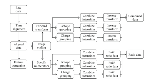
The Rosetta Elucidator uses raw mass spectroscopy (MS) data as an input and applies multiple normalizations and transformations in order to align, quantify, and compare features between samples. The steps of this process calculate three different types of data from the raw spectral input: aligned data, combined data, and ratio data. Aligned data have been converted into peak regions, or features, with corresponding intensity values that can be compared across samples. Combined data are composed of features with intensity values scaled by global mean intensities and transformed to stabilize error variance across samples. Ratio data are calculated through scaled intensity comparison between any two given sets of aligned data. The process is summarized in Figure 5 and described in the following.

Figure 5.

Diagram describing the general data processing steps Rosetta Elucidator use to calculate different data types out of raw, spectral input from a mass spectrometer (from Rosetta Inpharmatics LLC, Seattle, Wash, USA).

Data Alignment —

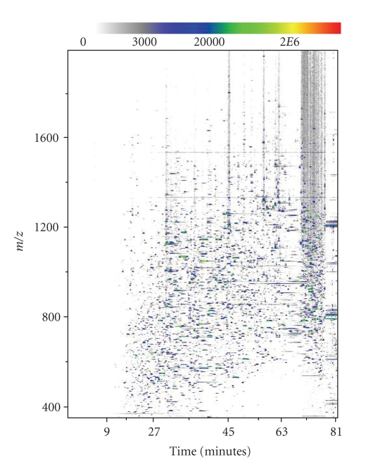
In its first stages, the Elucidator program transforms raw data into aligned data. Since peaks are not initially defined in the data, alignment starts at the level of the spectrum. The raw data for each sample include extremely precise mass to charge ratios (m/z ratios), times of elution from the liquid chromatogram, and detected intensity values for all ionized protein fragments. These values are converted into a pixelated image with an m/z axis, an elution time axis, and corresponding intensity values visualized with pixel color (Figure 6). From these raw MS images, a master image is chosen and all remaining raw images are aligned to that common spectrum. The main purpose of initial spectral alignment is to correct for variations in elution time that occur between MS runs. Shifting a spectrum in time to match a master image allows for meaningful comparison between corresponding peaks in different samples. Once this time-alignment has been executed, the noise and background of each image are removed to generate aligned data that can be viewed in the system.

Figure 6.

A 2D depiction of the raw MS data from the control-pre sample. The graph plots m/z versus elution time and displays intensity at a given point with color.

Feature Extraction —

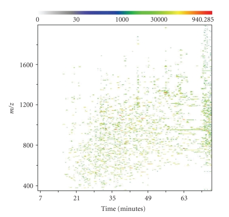
To extract meaningful peak regions, or features, from aligned data, a merged image is created from all the aligned images of the samples. To accomplish this, intensity values are averaged within treatment groups at each m/z and charge point. The resulting averaged treatment images are then averaged again across all treatments to generate a global merged image. Features can then be defined by overlaying ellipses or other two-dimensional shapes, called masks, to capture appropriate peak regions. The result across an experiment is a set of unique features with intensities measured by total ion current (TIC). Each individual feature represents a single isotopic mass peak from one of the charge states of a single peptide in a sample. Following feature extraction, the features can be grouped by isotope and the resulting isotope groups can be grouped by charge in order to capture all the features corresponding to a single peptide. An example of aligned data with extracted features is shown in Figure 7.

Figure 7.

A representation of aligned data features generated by Rosetta Elucidator from the control-pre mass spectrum. The m/z measurement from the mass spectrometer is plotted against the liquid chromatography elution time, with a scale of color depicting the intensity (total ion current or TIC) measured at each point. The Elucidator system defines features by mathematically identifying local intensity peak regions against background noise.

Combined Data —

Despite this extensive process, aligned data generated by the Rosetta Elucidator system is still not the most appropriate for the comparative questions we are addressing. Aligned data generated from multiple samples does not correct for certain experimental errors and variations that occur between runs. In order to generate the most meaningful data for comparison across samples, Rosetta Elucidator converts aligned data into combined data. The first step in this transformation is a form of intensity scaling that uses the mean intensity (or brightness) of a sample, possibly the mean average brightness of samples in a treatment group, and the mean average brightness across an entire experiment. The mean brightness of a sample is calculated by excluding any missing values and then averaging the lowest 90% of feature intensity values. Each intensity value is normalized by the mean intensity of its treatment condition and the global mean intensity across the experiment. This ensures that samples and treatments share a common mean intensity, further facilitating comparisons at the level of features, isotope groups, or charge groups. Following intensity scaling, the Elucidator system applies an error model-based transformation to stabilize the noise variance over the range of intensities in use. The transform function, shown below, converts the noise variance across all samples to a constant value:

$$\widehat{x}=\frac{\ln \hspace{0.17em}\left(b^2+2a^2\cdot x+2\sqrt{c^2+b^2\cdot x+a^2\cdot x^2}\right)}{a}+d,$$ (9)

where the a and b terms are related to the type of MS technology used. The a term is related to the fraction error of the instrument and the b term is related to the Poisson error of the instrument. In our experiment, we used a Linear Trap Quadrupole Orbitrab (LTQ-ORBI) mass spectrometer, which has a fraction error of 0.05 and a Poisson error of 15 000. The c term depends upon each feature's background value, which is an error model output for aligned data that calculates the background intensity surrounding the feature (ideally zero). An average of the background value is calculated over all features i and all treatments j in the experiment. The term d is related through a logarithm transform to a, b, and c. Following this forward transform, the transformed intensity values are averaged across all samples in the experiment to generate a separate combined intensity value. This combined intensity value is set apart from the individual sample intensity values and is calculated for later comparative and testing purposes. To generate the final combined data set, all intensities (including the combined intensity) must undergo an inverse transformation.

Ratio Data —

A final type of data, called ratio data, is calculated from two input sets of aligned data, one marked as a numerator and the other marked as a denominator. Ratio data is especially informative for our experiment because it provides a way to analyze relative intensity changes that occur across the same feature in different treatment groups as discussed below.

Feature Annotation —

With aligned data, combined data, and ratio data calculated automatically as part of our experimental design within Rosetta, we proceeded to annotate the sample features with the initial MS/MS peptide and protein identifications. All peptides with an Ion Score greater than 40, as calculated in Mascot search engine for peptide identification (Matrix Science Ltd., Boston, Mass, USA) were associated with their corresponding feature in Rosetta Elucidator.

3. Experimental Results

3.1. Dose-Volume RP Model

Data Exploration —

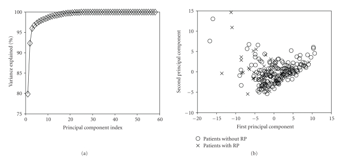
In Figure 8, we present PCA analysis of RP, with a pool of 58 variables. This pool included clinical variables (age, gender, race, chemo, stage, histology, treatment, etc.), dosimetric variables, such as V_x (volume getting at least x Gy), D_x (minimum dose to the hottest x% volume), and the relative location of the tumor within the lung. Notice that more than 93% of the variations in the input data were explained by the first two components (Figure 8(a)). Additionally, the overlap between patients with and without radiation pneumonitis is very high (Figure 8(b)), suggesting that there is no linear classifier that can adequately separate these two classes.

Figure 8.

Visualization of the 58 variables related to RP by PCA. (a) Variation explanation versus principle component (PC) index. This represents the variance of the data model about the mean prognostic input factor values. (b) Data projection into the first two components space. Note the high overlap in projection space, which suggests nonlinear kernel modeling to achieve better predictive power.

Kernel-Based Modeling —

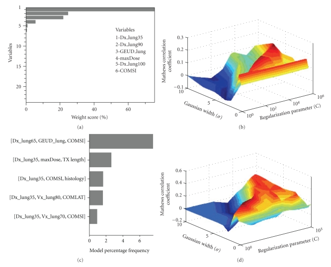
We first explored the effect of variable selection over the entire variable pool on the prediction of pneumonitis in the lung using support vector machine with a radial basis function kernel (SVM-RBF) as a classifier. In Figure 9(a), we show the top 30 selected variables using a recursive-feature-elimination SVM method, which was previously shown to be an excellent method for gene selection in microarray studies [31]. We used variable pruning to account for multicolinearity of correlated variables in this case. In Figure 9(b), we show the resulting SVM-RBF classifier using the top six variables (using a cutoff of 5% weighting score). The best MCC obtained was 0.22. In Figure 9(c), we show the results of variable selection using our previous multimetric approach based on model order selection and resampling with logistic regression [10, 19]. The model order was determined to be 3 with variables of D35, max dose, and COM-SI (center-of-mass of tumor location in the superior inferior direction) [35]. Figure 9(d) shows the evaluation results of applying the SVM methodology with RBF kernels using these selected variables. The resulting correlation (MCC = 0.34) on LOO testing data significantly improved our previously achieved multimetric logistic regression by 46%. The basic interpretation of this improvement is that the SVM automatically identified and accounted for interactions between the model variables. Despite the improvement, the model still does not achieve correlations levels that could be applied with high confidence in clinical practice. This is possibly because the model is unable to account for biological effects adequately, which we might need to incorporate as analyzed next.

Figure 9.

RP with a premodeling variable selection using (a), (b) the recursive feature elimination (RFE) method. Variables were chosen from a pool of 58 dosimetric, positional, and clinical variables. The top 23 variables selected by SVM-RFE are shown after applying a pruning step to correct for multicollinearity (RS = 0.75)(RS = 0.75). The top 6 variables (by applying a cutoff of 5% weighting score) were used for modeling pneumonitis. (b) An SVM-RBF classifier was tested on LOO data. (c), (d) Multimetric logistic regression approach. (c) The frequency of selected models order of 3 using our two-step resampling methods. The best-selected model consisted of three parameters (D35, COM-SI, and maximum dose). (d) The results of applying the SVM methodology with RBF kernels using these selected variables on LOO testing data. Note the improved performance in this case compared to RFE variable selection.

3.2. Proteomic Identification of RP

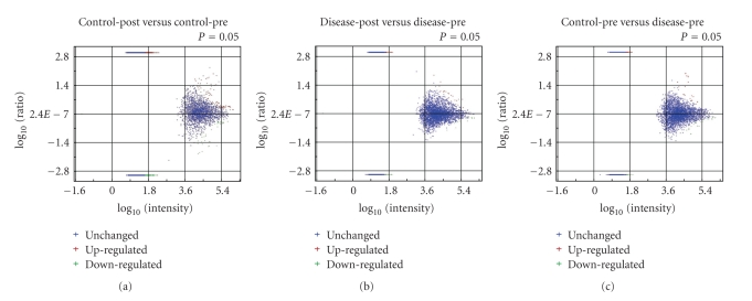
Using the 3-way methodology described in Section 2.7, we identified a group of features associated with RP by overlaying multiple subgroups of ratio data as follows. First, we organized subgroups of ratio data that displayed significant intensity changes between any two samples of interest. Significance was determined based on the P-value of each feature in a given set of ratio data. A P-value less than .05 was used as a cutoff. In this step, 11 979 unique features were identified after spectral alignment across the four samples. Of these 458 features directly matched, a peptide with an Ion Score >40 and 1289 features were annotated when direct peptide matches (with Ion Scores >40) were applied to all features in the same isotope group. Significant features could be further divided into upregulated and downregulated categories based on the sign of the fold change as shown in Figure 10.

Figure 10.

Categorization of upregulated and downregulated features for the ratio data as a function of average intensity for (a) control-post to control-pre, (b) Disease-post to disease-pre, and (c) control-pre to disease-pre.

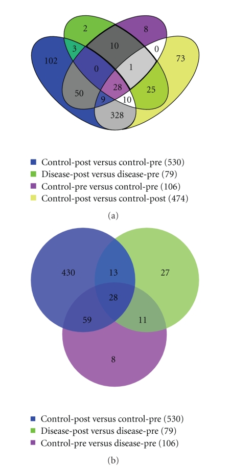
Secondly, features that significantly changed intensity between control-pre and control-post were overlaid with significant features that changed between disease-pre and disease-post. Shared features between these two datasets indicated candidate peptides that changed expression due to radiation. Alternatively, features unique to the disease-post versus disease-pre significant dataset were considered associated with a deleterious, hypersensitive reaction to radiation therapy, RP in our case. Using this hypersensitive dataset, we then overlaid the significant features from control-pre versus disease-pre. The features shared between these datasets are not only associated with RP, but also can be detected (due to differential concentrations) before treatment initiates. The results of these comparisons are summarized in the Venn diagrams of Figure 11.

Figure 11.

Diagram depicting the shared features between different sets of ratio data. The features in an individual set are those that displayed a significant change in intensity between the two members of the ratio. (a) All four samples, (b) the three ratios used to extract the RP candidates from the overlaid: control-pre to control-post, disease-pre to disease-post, and control-pre to disease-pre. Eleven features uniquely associated to a hypersensitive reaction as well as differential between patients before treatment.

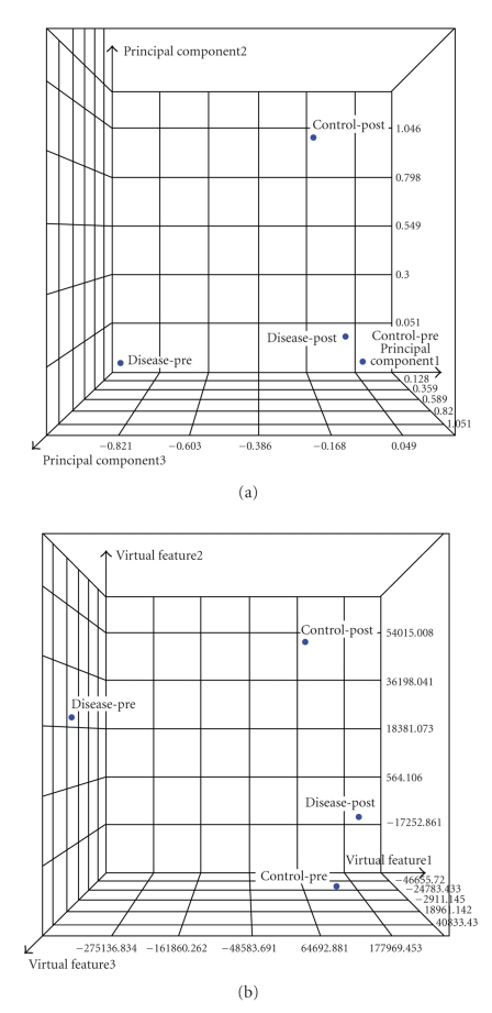
As noted from Figure 11(b), 41 features significantly changed after treatment in both patients. This can be attributed to regular radiation response. In addition, there were 489 significant features that were uniquely associated with the control case and 38 that were uniquely associated with the disease case. Eleven features were uniquely associated with a hypersensitive reaction as well as differential expression between patients before treatment, which represent our RP candidates. The relationship between these features and the original samples is represented in the PCA and MDS analyses of Figure 12. It is noticed that the separation between control-pre and disease-pre and disease-post and disease-pre is as anticipated from the experimental design strategy we followed to extract these features.

Figure 12.

Visualization of the candidate 11 features for RP (a) PCA and (b) MDS. Note the separation between control-pre and disease-pre and disease-post and disease-pre as anticipated from the experimental design strategy we followed to extract these features.

These 11 features were annotated as described in Section 2.7 and four proteins were identified as potential biomarkers for RP. All the identified proteins were downregulated postradiotherapy treatment and were known to play roles in inflammation responses. Two of these protein families were related to tissue remodeling, cognitive disorders, and fibrosis; one protein was part of the angiotensin-renin system, and the last protein seems to play a role in cytokine expression (interleukins and tumor necrosis factor).

4. Discussion

Modeling of radiotherapy outcomes constitutes a challenging problem due to the complex interaction between physical and biological factors. Better understanding of these relationships and the ability to develop predictive models of patients' treatment outcomes would lead to personalized treatment regimens. The tremendous increase in patient-specific clinical and biological information in conjunction with developing proper datamining methods and bioinformatics tools could potentially revolutionize the century old concepts of radiobiology and potentially improve the quality of care for radiation oncology patients.

In this work, we presented our methodology for making use of currently existing treatment planning archives to develop dose-volume models. We have demonstrated that supervised machine learning methods based on nonlinear kernels could be used to improve prediction of RP by a factor of 46% compared to traditional logistic regression methods. Potential benefits of these methods could be assessed based on PCA analysis of this data, where nonlinear kernels could be applied to resolve overlapping classes by mapping to higher-dimensional space [36]. We have applied resampling methods based on LOO to assess generalizabilty to unseen data and avoid overfitting pitfalls. Despite the gain in performance we attained from kernel methods, our results show that the best predictive model of RP has an MCC of 0.34 on LOO suggesting that our current variable space of clinical and physical dosimetric variables may not be adequate to describe the observed outcomes. This is despite the inclusion of high-order interaction terms using the SVM machinery. Therefore, we are currently exploring the inclusion of biological variables from peripheral blood draws to improve the prediction power of our RP model. Toward this goal, we have proposed a prospective study that builds upon our earlier retrospective analysis to delineate dose-volume effects in the onset of RP and include “missing” biological variables from minimally invasive clinical procedures inoperable NSCLC patients.

We have conducted a proteomic analysis of blood serum samples. Specifically, we have proposed a 3-way design strategy in order to distinguish between patient's variations, confounding radiation effects, and hypersensitivity predictors using intensity ratio changes. To test the validity of our design, PCA and MDS plots were used to measure separation between the samples in the estimated feature space. Our proteomic analysis was based on data from only two samples, but the results still provided promising candidates to validate with biochemical assays in a larger cohort. The entire study size of nineteen patients is an arguably small sample size as well, but according to our current protocol the number of patients in this study will increase every year, as new patients are recruited, with a final goal of 100–120 patients participating. Ongoing generation and validation of candidate proteins through additional mass spectrometry runs and extensive biochemical assays should provide increasingly interesting and accurate candidate proteins. Our feature selection strategy for candidate proteins is simplistic at this point, but we plan to make effective use of new emerging methodologies in statistical analysis of such data [37–40]. However, further investigation of datamining approaches to extract proper features and identify corresponding proteins with higher confidence from limited datasets is still required.

In our future work, we plan to further validate the derived proteins by examining their functional role by querying protein databases and measure their expression using Enzyme-Linked ImmunoSorbent Assay (ELISA). If successful, this data would be mixed with the developed dose-volume model using SVM-RBF and we will test the overall prediction on prospective data. Thus, we would be able to benefit from both retrospective and prospective data in our model building strategy.

5. Conclusions

We have demonstrated machine-learning application and a proteomics design strategy for building a predictive model of RP. The machine learning methods efficiently and effectively handle high-dimensional space of potentially critical features. We have applied this model successfully to interrogate dose-volume metrics. Our proteomics strategy seems to identify relevant biomarkers to inflammation response. Furthermore, we are currently investigating incorporation of these biomarkers into our existing dose-volume model of RP to improve its prediction power and potentially demonstrate its feasibility for individualization of radiotherapy of NSCLC patients.

References

- 1.American Cancer Society. Cancer Facts and Figures. Atlanta, Ga, USA: American Cancer Society; 2008. [Google Scholar]
- 2.Balter JM, Cao Y. Advanced technologies in image-guided radiation therapy. Seminars in Radiation Oncology. 2007;17(4):293–297. doi: 10.1016/j.semradonc.2007.06.001. [DOI] [PubMed] [Google Scholar]
- 3.Webb S. The Physics of Three Dimensional Radiation Therapy: Conformal Radiotherapy, Radiosurgery and Treatment Planning. Bristol, UK: Institute of Physics; 2001. [Google Scholar]
- 4.West CML, Elliott RM, Burnet NG. The genomics revolution and radiotherapy. Clinical Oncology. 2007;19(6):470–480. doi: 10.1016/j.clon.2007.02.016. [DOI] [PubMed] [Google Scholar]
- 5.Wouters BG. Proteomics: methodologies and applications in oncology. Seminars in Radiation Oncology. 2008;18(2):115–125. doi: 10.1016/j.semradonc.2007.10.008. [DOI] [PubMed] [Google Scholar]
- 6.Lea DE. Actions of Radiations on Living Cells. Cambridge, UK: Cambridge University Press; 1946. [Google Scholar]
- 7.Hall EJ, Giaccia AJ. Radiobiology for the Radiologist. 6th edition. Philadelphia, Pa, USA: Lippincott Williams & Wilkins; 2006. [Google Scholar]
- 8.Kirkpatrick JP, Meyer JJ, Marks LB. The linear-quadratic model is inappropriate to model high dose per fraction effects in radiosurgery. Seminars in Radiation Oncology. 2008;18(4):240–243. doi: 10.1016/j.semradonc.2008.04.005. [DOI] [PubMed] [Google Scholar]
- 9.Levegrün S, Jackson A, Zelefsky MJ, et al. Analysis of biopsy outcome after three-dimensional conformal radiation therapy of prostate cancer using dose-distribution variables and tumor control probability models. International Journal of Radiation Oncology, Biology, Physics. 2000;47(5):1245–1260. doi: 10.1016/s0360-3016(00)00572-1. [DOI] [PubMed] [Google Scholar]
- 10.El Naqa I, Bradley JD, Blanco AI, et al. Multivariable modeling of radiotherapy outcomes, including dose-volume and clinical factors. International Journal of Radiation Oncology, Biology, Physics. 2006;64(4):1275–1286. doi: 10.1016/j.ijrobp.2005.11.022. [DOI] [PubMed] [Google Scholar]
- 11.Levegrün S, Jackson A, Zelefsky MJ, et al. Fitting tumor control probability models to biopsy outcome after three-dimensional conformal radiation therapy of prostate cancer: pitfalls in deducing radiobiologic parameters for tumors from clinical data. International Journal of Radiation Oncology, Biology, Physics. 2001;51(4):1064–1080. doi: 10.1016/s0360-3016(01)01731-x. [DOI] [PubMed] [Google Scholar]
- 12.Marks LB. Dosimetric predictors of radiation-induced lung injury. International Journal of Radiation Oncology, Biology, Physics. 2002;54(2):313–316. doi: 10.1016/s0360-3016(02)02928-0. [DOI] [PubMed] [Google Scholar]
- 13.Deasy JO, Niemierko A, Herbert D, et al. Methodological issues in radiation dose-volume outcome analyses: summary of a joint AAPM/NIH workshop. Medical Physics. 2002;29(9):2109–2127. doi: 10.1118/1.1501473. [DOI] [PubMed] [Google Scholar]
- 14.Bentzen SM. From cellular to high-throughput predictive assays in radiation oncology: challenges and opportunities. Seminars in Radiation Oncology. 2008;18(2):75–88. doi: 10.1016/j.semradonc.2007.10.003. [DOI] [PubMed] [Google Scholar]
- 15.Kong F-M, Ten Haken R, Eisbruch A, Lawrence TS. Non-small cell lung cancer therapy-related pulmonary toxicity: an update on radiation pneumonitis and fibrosis. Seminars in Oncology. 2005;32(supplement 3):S42–S54. doi: 10.1053/j.seminoncol.2005.03.009. [DOI] [PubMed] [Google Scholar]
- 16.Chen Y, Okunieff P, Ahrendt SA. Translational research in lung cancer. Seminars in Surgical Oncology. 2003;21(3):205–219. doi: 10.1002/ssu.10039. [DOI] [PubMed] [Google Scholar]
- 17.Deasy JO, Blanco AI, Clark VH. CERR: a computational environment for radiotherapy research. Medical Physics. 2003;30(5):979–985. doi: 10.1118/1.1568978. [DOI] [PubMed] [Google Scholar]
- 18.El Naqa I, Suneja G, Lindsay PE, et al. Dose response explorer: an integrated open-source tool for exploring and modelling radiotherapy dose-volume outcome relationships. Physics in Medicine and Biology. 2006;51(22):5719–5735. doi: 10.1088/0031-9155/51/22/001. [DOI] [PubMed] [Google Scholar]
- 19.Deasy JO, El Naqa I. Image-based modeling of normal tissue complication probability for radiation therapy. In: Mehta M, Bentzen S, editors. Radiation Oncology Advances. New York, NY, USA: Springer; 2008. pp. 211–252. [PubMed] [Google Scholar]
- 20.Vapnik V. Statistical Learning Theory. New York, NY, USA: John Wiley & Sons; 1998. [Google Scholar]
- 21.El Naqa I, Bradley JD, Deasy JO. Machine learning methods for radiobiological outcome modeling. In: Mehta M, Paliwal B, Bentzen S, editors. In: Proceedings of the AAPM Symposium on Physical, Chemical and Biological Targeting in Radiation Oncology, vol. 14; July 2005; Seattle, Wash, USA. Medical Physics; pp. 150–159. [Google Scholar]
- 22.El-Naqa I, Yang Y, Galatsanos NP, Nishikawa RM, Wernick MN. A similarity learning approach to content-based image retrieval: application to digital mammography. IEEE Transactions on Medical Imaging. 2004;23(10):1233–1244. doi: 10.1109/TMI.2004.834601. [DOI] [PubMed] [Google Scholar]
- 23.El-Naqa I, Yang Y, Wernick MN, Galatsanos NP, Nishikawa RM. A support vector machine approach for detection of microcalcifications. IEEE Transactions on Medical Imaging. 2002;21(12):1552–1563. doi: 10.1109/TMI.2002.806569. [DOI] [PubMed] [Google Scholar]
- 24.Schèolkopf B, Tsuda K, Vert J-P. Kernel Methods in Computational Biology. Cambridge, Mass, USA: MIT Press; 2004. [Google Scholar]
- 25.Shawe-Taylor J, Cristianini N. Kernel Methods for Pattern Analysis. Cambridge, UK: Cambridge University Press; 2004. [Google Scholar]
- 26.Hastie T, Tibshirani R, Friedman JH. The Elements of Statistical Learning: Data Mining, Inference, and Prediction: With 200 Full-Color Illustrations. New York, NY, USA: Springer; 2001. [Google Scholar]
- 27.Haykin S. Neural Networks: A Comprehensive Foundation. 2nd edition. Englewood Cliffs, NJ, USA: Prentice-Hall; 1999. [Google Scholar]
- 28.Guyon I, Elissee A. An introduction to variable and feature selection. Journal of Machine Learning Research. 2003;3:1157–1182. [Google Scholar]
- 29.Kennedy R, Lee Y, van Roy B, Reed CD, Lippman RP. Solving Data Mining Problems through Pattern Recognition. Englewood Cliffs, NJ, USA: Prentice-Hall; 1998. [Google Scholar]
- 30.Dawson LA, Biersack M, Lockwood G, Eisbruch A, Lawrence TS, Ten Haken RK. Use of principal component analysis to evaluate the partial organ tolerance of normal tissues to radiation. International Journal of Radiation Oncology, Biology, Physics. 2005;62(3):829–837. doi: 10.1016/j.ijrobp.2004.11.013. [DOI] [PubMed] [Google Scholar]
- 31.Guyon I, Weston J, Barnhill S, Vapnik V. Gene selection for cancer classification using support vector machines. Machine Learning. 2002;46(1–3):389–422. [Google Scholar]
- 32.Matthews BW. Comparison of the predicted and observed secondary structure of T4 phage lysozyme. Biochimica et Biophysica Acta. 1975;405(2):442–451. doi: 10.1016/0005-2795(75)90109-9. [DOI] [PubMed] [Google Scholar]
- 33.Good PI. Resampling Methods: A Practical Guide to Data Analysis. 3rd edition. Boston, Mass, USA: Birkhäuser; 2006. [Google Scholar]
- 34.Härdle W, Simar L. Applied Multivariate Statistical Analysis. Berlin, Germany: Springer; 2003. [Google Scholar]
- 35.Hope AJ, Lindsay PE, El Naqa I, et al. Modeling radiation pneumonitis risk with clinical, dosimetric, and spatial parameters. International Journal of Radiation Oncology, Biology, Physics. 2006;65(1):112–124. doi: 10.1016/j.ijrobp.2005.11.046. [DOI] [PubMed] [Google Scholar]
- 36.El Naqa I, Bradley JD, Deasy JO. Nonlinear kernel-based approaches for predicting normal tissue toxicities. In: Proceedings of the 7th International Conference on Machine Learning and Applications (ICMLA '08); December 2008; San Diego, Calif, USA. pp. 539–544. [Google Scholar]
- 37.Zucht H-D, Lamerz J, Khamenia V, et al. Datamining methodology for LC-MALDI-MS based peptide profiling. Combinatorial Chemistry & High Throughput Screening. 2005;8(8):717–723. doi: 10.2174/138620705774962481. [DOI] [PubMed] [Google Scholar]
- 38.Gay S, Binz P-A, Hochstrasser DF, Appel RD. Peptide mass fingerprinting peak intensity prediction: extracting knowledge from spectra. Proteomics. 2002;2(10):1374–1391. doi: 10.1002/1615-9861(200210)2:10<1374::AID-PROT1374>3.0.CO;2-D. [DOI] [PubMed] [Google Scholar]
- 39.Nesvizhskii AI, Vitek O, Aebersold R. Analysis and validation of proteomic data generated by tandem mass spectrometry. Nature Methods. 2007;4(10):787–797. doi: 10.1038/nmeth1088. [DOI] [PubMed] [Google Scholar]
- 40.Broom BM, Do K-A. Statistical methods for biomarker discovery using mass spectrometry. In: Biswas A, Datta S, Fine JP, Segal MR, editors. Statistical Advances in Biomedical Sciences: Clinical Trials, Epidemiology, Survival Analysis, and Bioinformatics. Hoboken, NJ, USA: Wiley-Interscience; 2008. pp. 465–486. [Google Scholar]