Abstract
A system of ordinary differential equations is formulated to describe the pathogenesis of HIV infection, wherein certain features that have been shown to be important by recent experimental research are incorporated in the model. These include the role of CD4+ memory cells that serve as a major reservoir of latently infected cells, a critical role for T-helper cells in the generation of CD8 memory cells capable of efficient recall response, and stimulation by antigens other than HIV. A stability analysis illustrates the capability of this model in admitting multiple locally asymptotically stable (locally a.s.) off-treatment equilibria. We show that this more biologically-detailed model can exhibit the phenomenon of transient viremia experienced by some patients on therapy with viral load levels suppressed below the detection limit. We also show that the loss of CD4+ T-cell help in the generation of CD8+ memory cells leads to larger peak values for the viral load during transient viremia. Censored clinical data is used to obtain parameter estimates. We demonstrate that using a reduced set of 16 free parameters, obtained by fixing some parameters at their population averages, the model provides reasonable fits to the patient data and, moreover, that it exhibits good predictive capability. We further show that parameter values obtained for most clinical patients do not admit multiple locally a.s off-treatment equilibria. This suggests that treatment to move from a high viral load equilibrium state to an equilibrium state with a lower (or zero) viral load is not possible for these patients.
Keywords: HIV, immune response, censored data, inverse problems, model prediction, multiple equilibria
1 Introduction
Since the seminal work of Ho, et al., [20] demonstrated the promise for elucidating HIV disease mechanisms through mathematical modeling, a wide variety of models have been proposed to describe various aspects of in-host HIV infection dynamics (e.g., [1, 2, 3, 12, 17, 27, 28]). The most basic of these models typically include two or three of the key dynamic compartments: virus, uninfected target cells, and infected cells. These compartmental depictions lead to systems of linear or nonlinear ordinary differential equations in terms of state variables representing the concentrations in each compartment and parameters describing viral production and clearance, cell infection and death rate, treatment efficacy, etc. Solutions for the model states yield the time course of viral load and CD4+ counts, for example.
Although such models can be expected only to approximate the myriad processes underlying HIV pathogenesis, when used in conjunction with data as part of designed experiments, these models can be powerful tools in answering questions about the pathogenesis of HIV infection or similar biological processes. Mathematical models can also stimulate further clinical and laboratory research [28]. For example, early applications of linear systems to short-term data on patients undergoing ARV therapy suggested the now widely-held theory of very rapid and constant turnover of viral and infected cell populations [20, 27], contradicting previous assumptions that stable viral and CD4+ concentrations during the clinical latency period of chronic HIV infection are due to absence of significant viral replication.
While the model developed and analyzed here is new, it modifies and extends both conceptually and structurally the predictive model in [3]. That model included both CD4+/viral dynamics as in models discussed in [12] as well as immune response compartments whose importance have been earlier established [10, 26, 41] – see the discussions in [1]. However, since development of that model, important features of HIV pathogenesis have emerged. In particular, the key role of CD4+ memory cells as a latent reservoir for HIV has been clearly established in the experimental literature [18, 35]. As the authors in [35] note, even in treated patients who have had no detectable viremia for as long as 7 years, the latent reservoir decays so slowly that early initiation of Highly Active Anti-Retroviral Therapy (HAART) with the goal of virus eradication is not likely to succeed. Another important feature of HIV pathogenesis that has emerged is the critical role for T-helper cells in the generation of CD8 memory cells capable of an efficient recall response [4, 8, 21]. In any discussions of mathematical modeling of complex systems it is appropriate to point out that while complex models may be needed to provide accurate descriptions of the underlying dynamics, the models are most useful when they can be compared to clinical and/or experimental data and can also be used for prediction. In developing models for HIV infection and treatment or some other biological phenomenon, this requires a balance between complexity and utility.
Hence, in this paper we do not try to formulate a model that reflects all features of cellular immune response as well as all host and viral factors. Instead, we attempt to develop a model that can capture the most salient biological features of disease progression, one for which parameters can be plausibly estimated based on clinical data over long observation periods with treatment interruptions, one that has predictive capabilities, and one for which control/drug therapy design is tractable (e.g., one that exhibits multiple equilibria). Clinical data includes the usual measurements of CD4+ T-cell count and censored viral load, as well as new data that we will collect, such as HIV-specific CD8+ T-cell and phenotypic data (discrimination between naive, memory and effector T-cells).
The paper is organized as follows. In Section 2, a system of ordinary differential equations is developed to describe the pathogenesis of HIV and the cellular immune response. In Section 3 we discuss the ability of the model to admit multiple locally a.s. off-treatment equilibria. In Section 4 we demonstrate that one of the features of this more detailed biological model is the ability to exhibit the phenomenon of transient viremia following a non-HIV secondary infection, as proposed and demonstrated by others [22]. Furthermore, the phenomenon of transient viremia is used to elucidate the role of latently-infected CD4+ memory cells and the effect of CD4+ help on CD8+ memory during the ensuing immune response. In Section 5 the expectation maximization algorithm leading to weighted least-squares techniques is employed to fit the model to clinical data with lower limit censoring. The predictive capability of the model is also investigated by using simulation results, with parameters estimated from only half of the longitudinal observations, to predict the immune response in the latter half and comparing these predictions to clinical observations. In Section 6 we use the parameter estimates obtained in Section 5 to predict the number of off-treatment infected and uninfected equilibrium states available to each patient. Finally we close with conclusions and remarks in Section 7.
2 HIV Model
The model we develop in this paper conceptually modifies and extends the model in [3], wherein two types of target cells (CD4+ T-cells and macrophages), along with their corresponding infected states, free virus, and immune effector cells (CTL) are included in the model. Clinical data fitting results show that the preliminary model of [3] provides reasonable fits to most patient data and has impressive predictive capability when comparing model simulations, with parameters based on estimation using only half of the longitudinal observations, to the full longitudinal data sets. However, that model does not incorporate some important features of HIV pathogenesis and the cellular immune response, such as CD4+ memory cells as the major reservoir of latently infected cells and a critical role for T-helper cells in the generation of CD8 memory cells capable of an efficient recall response. To incorporate these important features, we thus seek a model that includes some measure of CD4+ T-helper cells, infected memory CD4+ T-cells and HIV-specific memory CD8+ T-cells. To retain the simplicity of the model, secondary target cells, such as macrophages, are not included as a compartment in our new model. It is worth noting that omitting the secondary target cells should not affect our clinical data fitting and predictive capabilities since this type of cell, even though it is very important at the beginning of infection, does not contribute significantly to the virus pool in the long run [19]. The model compartments are illustrated in Table 1, wherein the resting CD4+ T-cells (T2) are assumed to include naive CD4+ T-cells and memory CD4+ T-cells. This is reasonable since these two types of cells have similar behavior such as longer life spans and distribution in the lymphoid tissue. Once these resting CD4+ T-cells become activated, either through antigen priming of naive cells or reactivation of memory cells, they are more susceptible to HIV infection than resting cells and suffer elevated mortality [14]. Hence, we include these activated naive cells and reactivated memory cells in the other compartment as activated CD4+ T-cells (T1). Infected resting and activated cells are represented by the and states, respectively. A schematic of this new model is depicted in Fig. 1.
Table 1.
Model States.
| states | unit | description |
|---|---|---|
| T 1 | cells/μl-blood | uninfected activated CD4+ T-cells |
| cells/μl-blood | infected activated CD4+ T-cells | |
| T 2 | cells/μl-blood | uninfected resting CD4+ T-cells |
| cells/μl-blood | infected resting CD4+ T-cells | |
| VI | RNA copies/ml-plasma | infectious free virus |
| VNI | RNA copies/ml-plasma | non-infectious free virus |
| E 1 | cells/μl-blood | HIV-specific effector CD8+ T-cells |
| E 2 | cells/μl-blood | HIV-specific memory CD8+ T-cells |
Figure 1.
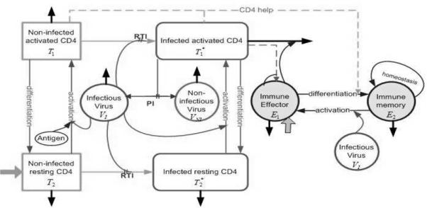
Flow chart of model (2.1) with compartments as described in Table 1. Solid black arrows indicate death/clearance, solid gray arrows indicate birth/input. PI and RTI denote protease inhibitor and reverse transcriptase inhibitor, respectively.
The corresponding compartmental ordinary differential equation (ODE) model for in-host HIV infection dynamics is based on balance laws and is given by
| (2.1) |
with an initial condition vector
Here the factors 103 are introduced to convert between microliter and milliliter scales, preserving the units from some of the earlier published papers [1, 10]. The treatment factors ξ1(t) = ε1u(t) and ξ2(t) = ε2u(t) represent the effective treatment impact, consisting of efficacy factors ε1 modeling the relative effectiveness of reverse transcriptase inhibitor (RTI), ε2 describing the relative effectiveness of protease inhibitor (PI), and a time-dependent treatment function u(t) (0 ≤ u(t) ≤ 1) representing HAART drug level, where u(t) = 0 is fully off and u(t) = 1 is fully on. Since HIV treatment is nearly always administered as combination therapy, we do not consider the possibility of monotherapy, even for a limited period of time, though this could be implemented by considering separate treatment functions.
Since the T2 compartment includes naive CD4+ T-cells, the input term for T2 compartment is used to account for the source rate of naive CD4+ T-cells. This term depends on the viral load level since the thymus production can be diminished if the viral load is too high [24]. To limit the introduction of additional parameters, we assume that uninfected and infected resting CD4+ T-cells (T2 and , respectively) have the same natural death rate d2. We remark that activated CD4+ T-cells have a higher natural death rate than resting memory and naive cells, and we use d1 to denote the natural death rate of uninfected activated CD4+ T-cells T1. The immune effector cells E1 remove infected activated cells CD4+ T-cells from the system by cell lysis with a rate m. However, immune effector cells do not remove infected resting cells , since these cells are in a quiescent state where the virus is not replicating and, thereby, escape the detection of the immune effector cells. These infected resting cells are assumed to become targets for lysis only after activation [9].
The infected activated cells result from encounters between uninfected activated cells T1 and free infectious virus VI with infection rate k1. The resulting term k1V1T1 is modified by a factor 1 – ξ1(t) to account for RTI treatment. Infection of the resting T-cell compartment T2, which is comprised of both memory and naive CD4+ T-cells, can occur in a number of ways. First, the most commonly transmitted R5 virus form of HIV-1 that utilize the chemokine receptor CCR5 can enter a subset of resting memory cells that express sufficient levels of CCR5 to support infection [9]. In addition, the X4 form of the virus can infect resting CD4+ T-cells, whether they belong to the naive or memory subsets. However, infection of naive and memory cells through these routes occurs much less frequently than infection of T1, and, once infected, these cells often do not progress to a long-term stably-infected state in which the virus is integrated into the host DNA. In addition, it has been shown that infected naive CD4+ T-cells do not significantly contribute to the pool of infected resting CD4+ T-cells [11]. Hence, the term (1 – fξ1(t))k2VIT2 is used to represent the infection process that results from encounters between the uninfected resting CD4+ T-cells and free virus VI, but with an infection rate k2 < k1 to account for a significantly lower rate of infection as compared to activated CD4+ T-cells. The treatment factor ξ1(t) is potentially more effective in T1 than in T2, where the efficacy is modelled by fξ1(t) with 0 ≤ f ≤ 1.
A much more stable form of latent infection arises when activated CD4+ T-cells that have integrated HIV-1 DNA survive long enough to revert back to resting memory state, and latently infected resting CD4+ T-cells with integrated HIV-1 DNA are present in all infected individuals but only at low frequency [9, 15]. Hence, the terms involving are included in the model to account for the phenomenon of differentiation of infected activated CD4+ T-cells into infected memory or resting CD4+ T-cells at rate γT. For simplicity, the rate at which uninfected activated CD4+ T-cells T1 differentiate into uninfected resting CD4+ T-cells T2 is also assumed to be γT; the model could be extended easily to the case with different differentiation rates.
As the authors of [9] concluded, there is turnover (activation) in the latent reservoir when patients are viremic and the degree of turnover depends on the level of viremia. We thus assume that the activation of infected HIV-specific resting CD4+ T-cells depends on the virus concentration with a half-saturation constant KV. Hence, the terms involving are used to represent the activation of infected HIV-specific resting CD4+ T-cells with maximum activation rate of aT. Again to preserve the simplicity of this model, we assume that activation of uninfected HIV-specific resting CD4+ T-cells T2 also depends on the virus concentration, with a half saturation constant KV, and that the maximum activation rate is also aT. Thus, the terms involving represent the activation of uninfected HIV-specific resting CD4+ T-cells. In order to incorporate the activation of resting CD4+ T-cells by some non-HIV antigen and preserve the simplicity of the model, we include the simple terms aAT2 and into our model to describe this phenomenon, with aA being the activation rate by non-HIV antigen. The parameter aA here can be utilized as a constant to represent a chronic level of infection or as a function of time t to describe infections that are cleared by the body. These activation terms represent losses to the T2 and compartments, with corresponding gain terms for the T1 and compartments. However, the gain terms for T1 and include a multiplicative factor pT to account for the net proliferation due to clonal expansion and programmed contraction. For simplicity, we assume that uninfected and infected CD4+ T-cells have the same expansion factor pT; again this can be readily extended to include processes with different expansion factors.
Virus in the reservoir of infected resting CD4+ T-cells is latent and no virus can be produced by these cells unless they are activated [9]. Hence, free virus particles VI are produced only by activated infected CD4+ T-cells during viral budding leading up to viral produced lysis of the CD4+ T-cells. The parameter NT accounts for the number of RNA copies produced during this process in the viral source term . In addition to a natural clearance rate c, we also include term in the free virus compartment V to account for the removal of free virus that takes place when free virus infects T1 and T2. We make the simplifying assumption that , i.e., one free virus particle is responsible for each new infection. This could be adapted easily for multiple virus particles being responsible for each new infection by choosing ρi > 1. Since clinical measurements of viral load do not differentiate between infectious and non-infectious virus, we include a compartment in the model for tracking the amount of non-infectious virus VNI (viral load VL = VI + VNI). The action of a protease inhibitor, resulting in the production of non-infectious virus VNI by infected cells is modeled by ξ2. It should be noted that the inclusion of this additional state does not affect the dynamics of the other state variables, but its inclusion is necessary in order to use the clinical data for the total viral load VL in our inverse problem methodology below.
The source term λE, the constant death term δE1, and the nonlinear infected cell-dependent birth and death terms in the E1 compartment are adopted from the model in [2, 3], where the authors suggested that, by including such terms in the immune effector compartment, the model can admit multiple stable off-treatment steady states and exhibit transfer between “healthy” and “unhealthy” locally stable steady states via optimal or suboptimal structure treatment interruptions (STI) therapies. This makes it a good candidate for our investigation. Memory CD8+ T-cells are also subject to strict homeostatic control [36]; background expansion of memory cells through intermittent cell division being countered by an equivalent level of cell death. Hence, we include the term for homeostatic regulation in the E2 compartment, similar to that used in [39]. In the homeostatic regulation, bE2 represents the maximum proliferation rate and δE2 corresponds to the death rate, where the proliferation signal decreases linearly with population size.
The term in the model is used to include the essential role that activated CD4+ T-cells play in the generation of memory CD8+ T-cells, where parameter Kγ is a half-saturation constant and γE is the maximum rate at which E1 differentiates into E2. Since depletion of CD4+ cells has a minimal effect during the recall response [34, 40], the term for reactivation of memory CD8+ T-cells is independent of CD4+ T-cell help. Similar to the activation of HIV-specific resting CD4+ T-cells, we assume that activation of HIV-specific memory CD8+ T-cells also depends on the virus concentration. For simplicity, we use the same half-saturation constant KV for the activation of memory CD8+ T-cells. Since CD8+ T-cells tend to divide sooner and to have a faster rate of cell division than CD4+ T-cells [33], we use a different parameter pE to account for the net proliferation due to clonal expansion and programmed contraction of activated CD8+ T-cells in the E1 compartment.
3 off-treatment Stability Analysis
Our model choice is partly motivated by its admission of multiple locally a.s. off-treatment equilibria (corresponding to ε1 = 0 and ε2 = 0), which is important in the sense that we seek to investigate the possibility of improvement of long-term health by using STI during acute infection to affect a change from an “unhealthy” equilibrium to a “healthy” one. A general analysis of the equilibria of the model (2.1) and their stability properties is challenging due to the complexity of the system and is generally not solvable in analytic form. Hence, in this section we illustrate the existence of multiple locally a.s. equilibria through specific examples and numerically investigate the behavior of these equilibria with respect to changes in parameters and initial conditions.
Uninfected equilibrium in the absence of non-HIV infection (aA = 0)
In the absence of non-HIV antigen (aA = 0), it is easy to see that model (2.1) has the following off-treatment uninfected equilibrium:
| (3.1) |
Substituting the above equilibrium into the Jacobian matrix of model (2.1), we find that the eigenvalues of this matrix are given by –(δδE1 + mλE + γT δE1)/δE1, –c, –d2, –d2, –(cd2 + 1000k2δT)/d2, –δE1, bE1, δE2 – δE2 and – γT. Hence, if bE2 < δE2 then all the eigenvalues of this Jacobian matrix are negative, which implies that under this case equilibrium (3.1) is locally a.s. On the other hand, if bE2 > δE2, then we obtain a different uninfected equilibrium:
| (3.2) |
In this case, we find that the eigenvalues of Jacobian matrix are given by (δδE1 + mλE + γTδE1)/δE1, –c, –d1 – γT, –(cd2 + 1000k2λT)/d2, –δE1, –δE2(bE2 – δE2)/bE2, –d2 and –d2. Hence, equilibrium (3.2) is also locally a.s. Therefore, for the case aA = 0 model (2.1) always has a locally a.s. off-treatment uninfected equilibrium. The existence of a locally a.s. uninfected equilibrium is biologically reasonable in light of research documenting the existence of some sex workers and health-care workers who, though exposed to HIV-contaminated body fluids, remain HIV-negative [30, 31]. We note that this feature of our new model is not present in the earlier model investigated in [3].
Multiple equilibria in the absence of non-HIV infection (aA = 0)
We next illustrate the existence of multiple equilibria with specific examples when aA = 0 and the values of all the other parameters as specified in Table 2, unless otherwise stated. Since values for most of the parameters in this model can not be found in the literature, the values listed in Table 2 are chosen for model illustration purposes. When determining equilibria for this complex model there are usually many unstable or physically-meaningless (eg., negative state values) equilibria. In the discussion that follows, unless otherwise stated, we focus our attention on the locally a.s., physically-meaningful equilibria only.
Table 2.
Parameter values used in model (2.1) to illustrate the existence of multiple equilibria. Note that for this parameter set bE2 < δE2.
| parameter | value | parameter | value | parameter | value |
|---|---|---|---|---|---|
| d 1 | ε 1 | ∈ [0, 1] | k 1 | ||
| δ | m | λ T | |||
| d 2 | KV | Ks | |||
| f | 0.34 | γ T | NT | ||
| ε 2 | ∈ [0, 1] | c | λ E | ||
| bE 1 | dE | Kb 1 | |||
| aA | δ E 1 | Kd | |||
| aT | pT | 1.2 | k 2 | ||
| aE | pE | 3 | Kγ | ||
| γ E | bE 2 | Kb 2 | |||
| δ E 2 |
In particular, we wish to explore the effect that CD4+ memory cell activation plays on the equilibrium states available to the system. Since, for economy, we have included both naive and memory cells in a single resting CD4+ T-cell compartment T2 (or for the infected case), the activation factor represents both activation of naive cells and the reactivation of memory cells. In the limit of large VI the maximum activation rate is aT. In the treatment that follows, we examine the role of aT on the equilibrium states available to the system. We first examine the off-treatment equilibria (listed in Table 3) for the case aT = 8 × 10⁻³ day−1. We can see that in this and each of the other two cases we consider, there is an uninfected equilibrium similar to the one in (3.1), which we designate as EQ1. In addition to the uninfected equilibrium, we have two infected equilibria, designated as EQ2 and EQ3, where EQ2 represents a “healthy” steady state with immune control of the viral infection, restoration of CD4+ T-cell counts (915.6 cells/μl-blood), and a strong CD8+ immune response (897.5 cells/μl-blood). Equilibrium EQ3 represents an “unhealthy” steady state corresponding to a dangerously high viral load set point, lower CD4+ T-cell counts (445.8 cells/μl-blood), and a much lower CD8+ immune response (0.04860 cells/μl-blood).
Table 3.
Off-treatment steady states for model (2.1) with aA = 0 day−1, aT = 8 × 10⁻³, 8 × 10⁻², and 1 × 10⁻³ day−1, and the values of all the other parameters as specified in Table 2. Non-physical and unstable steady states are omitted.
| aT |
||||||
|---|---|---|---|---|---|---|
| 8 × 10⁻³ |
8 × 10⁻² |
1 × 10⁻³ | ||||
| state | EQ1 | EQ2 | EQ3 | EQ2 | EQ3 | EQ2 |
| T 1 | 0 | 184.3 | 13.13 | 352.1 | 13.12 | 40.27 |
| 0 | 0.05621 | 5.330 | 0.05582 | 7.659 | 0.05935 | |
| T 2 | 1400 | 731.2 | 424.4 | 142.8 | 59.36 | 1247 |
| 0 | 0.04393 | 2.984 | 0.005110 | 0.4801 | 0.1187 | |
| VI | 0 | 265.1 | 28410 | 236.5 | 40830 | 310.0 |
| VNI | 0 | 0 | 0 | 0 | 0 | 0 |
| E 1 | 0.01 | 799.2 | 0.04574 | 1422 | 0.03872 | 140.0 |
| E 2 | 0 | 98.32 | 0.002863 | 184.5 | 0.002520 | 14.07 |
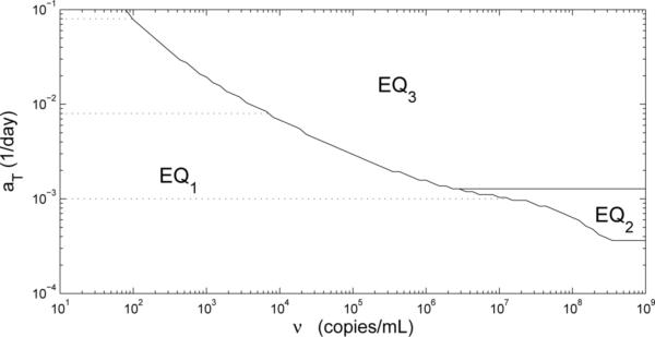
If we begin simulations with the initial conditions (0, 0, 1400, 0, ν, 0, 0.01, 0), i.e., a nontrival amount ν of infectious free virus, then the solution of model (2.1) converges to either the uninfected equilibrium EQ1 or the “unhealthy” infected equilibrium EQ3 (see Fig. 2). The particular steady state that the model converges to depends on the viral load level ν. Simulation results reveal that the solution will not converge to EQ3 until the value of ν is close to 6576 copies/ml-plasma.
Figure 2.
Phase diagram showing equilibrium attained as a function of the initial viral load ν and the parameter aT. It should be emphasized that this plot is only applicable for the particular initial condition (0, 0, 1400, 0, ν, 0, 0.01, 0).
If we set the value of aT larger, such as 8 × 10⁻² day−1, and keep the values of all the other parameters the same, then we still have three locally a.s. off-treatment equilibria: uninfected, “healthy” infected and “unhealthy” infected, where the uninfected equilibrium is the same as before (Table 3). However, the “unhealthy” infected equilibrium (EQ3) in this case has a higher viral load, a much lower CD4+ T-cell count (80.62 cells/μl-blood), and a lower immune response (0.04124 cells/μl-blood) than the EQ3 when aT = 8 × 10⁻³ day−1. Even though the “healthy” infected equilibrium EQ2 has a slightly lower viral load level and a much higher CD8+ immune response (1607 cells/μl-blood) than the EQ2 when aT = 8 × 10⁻³ day−1, it has degraded with respect to the CD4+ T-cell count (495.0 vs. 915.6 cells/μl-blood).
If we now start simulations with aT = 8 × 10⁻² day−1 and the initial conditions (0, 0, 1400, 0, ν, 0, 0.01, 0), then the solution of model (2.1) also converges to either uninfected equilibrium or “unhealthy” infected equilibrium depending on ν. But in this case, the solution converges to its corresponding “unhealthy” infected equilibrium with ν around 100.3 copies/ml-plasma (see Fig. 2). Hence, the viral load necessary for infection depends on the maximum activation rate aT; low values of aT require a larger viral load to reach an infected state. Furthermore, when infected, smaller values of aT produce “healthier” infections than infections with larger aT values, in terms of CD4+ T-cell counts and viral load level.
If we set the maximum activation rate of resting CD4+ T-cells lower, such as aT = 1 × 10⁻³ day−1, and keep the values of all the other parameters to be the same as those illustrated in Table 2, then we find that we have only two locally a.s. off-treatment equilibria: the uninfected steady state (EQ1) and “healthy” infected steady state (EQ2), where again the uninfected steady state is the same as with aT = 8 × 10⁻³ day−1 (Table 3). Even though the “healthy” infected steady state has a higher viral load level (310 copies/ml-plasma) and lower immune response (154 cells/μl-blood) than it does when aT = 8 × 10⁻³ day−1, the immune response still controls the viral load to maintain it below a detection limit of 400 copies/ml-plasma. This equilibrium also has much higher CD4+ T-cell counts (1290 cells/μl-blood) than the case when aT = 8 × 10⁻³ day−1. If we start the simulation with the initial conditions (0, 0, 1400, 0, ν, 0, 0.01, 0), then the solution of model (2.1) converges either to its uninfected equilibrium or “healthy” infected equilibrium based on the value of ν, and it converges to this “healthy” infected equilibrium with ν around 1.527 × 10⁷ copies/ml-plasma (Fig. 2).
The examples above demonstrate the existence of multiple off-treatment equilibria and illustrate that changing the value of a parameter, such as the maximum activation rate aT, has an effect on both the number and “health” characterization of the equilibria. In addition, the initial conditions of the system determine which equilibrium is attained after initial infection. Across a population, the parameter values can be expected to vary to represent different host factors and host-virus interaction rates. In the analysis of parameter aT, we find that a person with a lower aT value requires a larger viral load in order to get infected and, once infected, attains a “healthier” set point outcome, in terms of their CD4+ T-cell counts and viral load level, than those with higher values of aT. Analysis with other parameters, such as the expansion factor pT, reveals similar behavior.
Multiple equilibria in the presence of non-HIV infection (aA ≠ 0)
In order to investigate whether the activation due to a non-HIV antigen can affect the number of physical equilibria and their local asymptotic stability, we performed simulation with aA = 10−5 day−1 and the values of all the other parameters as specified in Table 2. All the locally a.s., physical, off-treatment equilibria are tabulated in Table 4, which indicates that we still have three locally a.s. equilibria: an uninfected steady state EQ1, a “healthy” infected steady state EQ2 and an “unhealthy” infected steady state EQ3. We also observe that EQ1 has a nonzero E2 even though bE2 < †E2 and a nonzero T1, which is not observed for equilibrium EQ1 where aA = 0 (Table 3). Otherwise, the equilibria for the two cases (aT = 8 × 10⁻³ day−1 and aA = 0 or 1 × 10⁻⁵ day−1) are very similar.
Table 4.
Off-treatment steady states for model (2.1) with aA = 1 × 10⁻⁵ and 1 × 10⁻² day−1 and the values of all the other parameters as specified in Table 2. Non-physical and unstable steady states are omitted, except in the case of EQ1 when aA = 1 × 10⁻² day−1, which is unstable. Note that aT = 8 × 10⁻³ day−1 for this analysis.
| aA |
||||||
|---|---|---|---|---|---|---|
| 1 × 10⁻⁵ |
1 × 10⁻² |
|||||
| state | EQ1 | EQ2 | EQ3 | EQ1 | EQ2 | EQ3 |
| T 1 | 0.6710 | 184.5 | 13.13 | 266.7 | 277.2 | 13.12 |
| 0 | 0.05621 | 5.332 | 0 | 0.05592 | 6.567 | |
| T 2 | 1398 | 730.6 | 424.0 | 555.6 | 404.2 | 228.2 |
| 0 | 0.04388 | 2.982 | 0 | 0.01835 | 1.777 | |
| VI | 0 | 265.0 | 28420 | 0 | 248.2 | 35010 |
| VNI | 0 | 0 | 0 | 0 | 0 | 0 |
| E 1 | 0.009938 | 799.9 | 0.04573 | 0.009121 | 1160 | 0.04113 |
|
E
2
|
0.001562 |
98.41 |
0.002862 |
0.02198 |
147.6 |
0.002630 |
| local stability | a.s. | a.s. | a.s. | unstable | a.s. | a.s. |
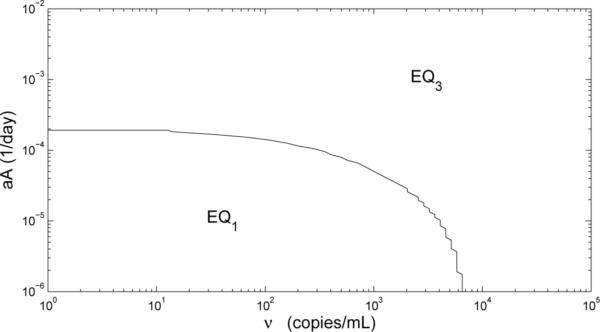
If we start simulations with the initial conditions (0.6710, 0, 1398, 0, ν, 0, 0.009938, 0.001562), then the solution of model (2.1) converges either to its uninfected equilibrium EQ1 or “unhealthy” infected equilibrium EQ3 based on the value of ν, and it will not converge to EQ3 until ν is close to 4000 (Fig. 3), as compared to 6576 copies/ml-plasma when aA = 0. Hence, a person infected with a non-HIV virus becomes HIV-infected at lower viral loads than when no other infection is present.
Figure 3.
Phase diagram showing equilibrium attained as a function of the initial viral load ν and the parameter aA. Initial conditions for simulations, corresponding to the uninfected equilibrium EQ1, are calculated for each value of aA. Note that aT = 8 × 10⁻³ day−1 for these simulations.
If we take the value of aA larger, such as aA = 1 × 10⁻² day−1, then the uninfected equilibrium is no longer stable, but we still have the locally a.s. “healthy” and “unhealthy” steady states designated as EQ2 and EQ3 in Table 4, respectively. If we start simulations with the initial conditions (266.7, 0, 555.6, 0, ν, 0, 0.009121, 0.02198), then the solution of model (2.1) converges to EQ3, regardless of the initial viral load ν (Fig. 3). This means that when the system is in the state EQ1, introduction of even the smallest amount of virus will cause the system to converge to the “unhealthy” equilibrium EQ3.
Furthermore, Table 4 indicates that as the activation rate by non-HIV antigen aA becomes larger, the locally a.s. “healthy” steady state has degraded, in terms of the total CD4+ T-cells counts (915.1 vs. 681.1 cells/μl-blood), while the viral load has improved (265.0 vs. 248.2 copies/ml-plasma), as well as the immune response (898.4 vs. 1307 cells/μl-blood). In addition, the locally stable “unhealthy” steady state has worsened, in terms of a much lower CD4+ T-cell count (445.4 vs. 249.4 cells/μl-blood), higher viral load set point (28420 vs. 35010 copies/ml-blood), and lower immune response (0.04859 vs. 0.04376 cells/μl-blood). Therefore, at this point increasing aA leads to similar behavior as does increasing aT when aA = 0.
The examples above summarize an investigation as to the effect of a non-HIV infection (aA ≠ 0) on the outcome of an HIV-infection. We find that a person with a non-HIV infection (aA ≠ 0) requires a smaller initial viral load ν to sustain an HIV infection and, once infected, attains a worse outcome, in terms of CD4+ T-cell counts and viral load levels, than a person without a non-HIV infection (aA = 0). We find that multiple equilibria, including an uninfected equilibrium, exist in the presence of a small non-HIV infection (aA = 1 × 10⁻⁵ day−1). However, for larger levels of non-HIV infection (aA = 1 × 10⁻² day−1), the uninfected equilibrium is unstable and even the smallest initial viral load×will lead to an “unhealthy” equilibrium state (Fig. 3).
4 Transient Viremia
Adherence to a regimen of HAART suppresses the viral loads of most infected HIV patients below the level of detection (<400 or <50 copies/ml-plasma depending on the assay used) by standard assays . However, a number of these well-suppressed patients experience unexplained “viral blips” or transient viremia while on therapy [16, 22]. In a study [16] of 123 patients, these viral blips are estimated to have a duration of approximately two to three weeks with a mean blip amplitude of 158 ± 132 copies/ml-plasma. Furthermore, it is observed that the blip frequency inversely correlates with CD4+ T-cell counts. In this section, we investigate how infection with a non-HIV antigen can lead to transient viremia for those patients who are on treatment and have successfully suppressed their viral loads to undetectable levels. To do so, we use the states of a locally a.s. “healthy” infected equilibrium (201, 0.056, 730, 0.040, 288, 0, 240, 29.2), corresponding to ε1 = 0.7, ε2 = 0, aA = 0, and the values of all the other parameters as specified in Table 2, as the initial conditions for simulations in which we allow parameter aA to be a function of time t, while keeping all other parameter values to be the same. As we drive the system (2.1) with the non-HIV infection aA(t) we monitor the states of the system, particularly the viral load. While the cause of viral blips has not yet been resolved, one proposed mechanism [22] posits that viral blips could be due to an increase in activated CD4+ cells as a result of secondary infection or vaccination. Our approach, introducing a time-dependent non-HIV infection aA(t) is consistent with this proposed mechanism and demonstrates that our model supports such a scenario.
Transient viremia caused by a single non-HIV infection
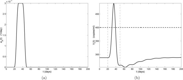
Figure 4(a) illustrates the case of a one-time non-HIV infection occurring on days 20 through 50, with a peak value of 0.003 day−1 (days 30 to 40). Figure 4(b) depicts the HIV viral progression VI(t) resulting from this infection. In Fig. 4(b) we see that there is a small delay before the viral load begins to increase. This delay is reasonable since there is no activation term (aA) in the VI compartment of model (2.1) and the viral load can only increase after increases. About 10 days after the start of the infection (day 30), the viral load rises above the detection limit (400 copies/ml-plasma), reaching its peak value 15 days post-infection (day 35). This viral blip drops below the detection limit 20 days post-infection (day 40), before the infection has completely cleared.
Figure 4.
(a) Activation rate aA(t) by a non-HIV antigen. The duration of the infection is 30 days; (b) Viral load VI(t) (solid line), censored data level (horizontal dashed line), and infection start and stop times (vertical dash-dot lines).
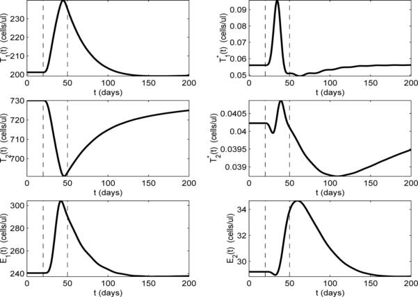
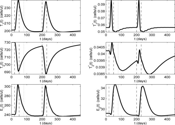
To further investigate the dynamics of transient viremia, we plot the other model compartments for the example shown in Fig. 4 (we omit compartment VNI, since, with ε2 = 0 and VNI(0) = 0, VNI ≡ 0). In Fig. 5, it can be seen that the T-cell compartments (T1, , T2, and ) respond at the start of the infection (day 20). This is not surprising because the non-HIV antigen activation term aA appears in the dynamical equations for these compartments in model (2.1). It is also reasonable that the resting (naive and memory) T-cell compartments (T2 and ) initially decrease, while the activated T-cell compartments (T1 and ) increase, since, at the start of the infection, resting cells are reactivated (memory) to fight the infection or activated through infection (naive). There is also a short delay between the peak value of and the peak value of which is likely due to the time delay in the differentiation of into . Comparing compartment of Fig. 5 with compartment VI in Fig. 4, we find that these two compartments exhibit very similar time-dependent behavior. Again, this is to be expected because the only compartment that produces virus is .
Figure 5.
Model dynamics with ε1 = 0.7, ε2 = 0, and the values of all the other parameters as specified in Table 2. Activation rate by a non-HIV antigen aA(t) is as depicted in Fig. 4(a). Vertical dashed lines indicate the start and stop times of the non-HIV infection.
If we focus our attention on the uninfected T-cell compartments (T1 and T2 in Fig. 5), we see that the peak of T1 corresponds to the valley of T2. The fact that T1 increases and T2 decreases for most of the infection implies that the effects of the activation terms pT (aTVI/(VI + KV) + aA)T2 and (aTVI/(VI + KV) + aA)T2 dominate over the differentiation terms γTT1 and other loss terms in model (2.1) during the infection. That is, the T2 compartment is losing more through activation than it is gaining through differentiation of T1, and vice versa for T1. The situation is reversed as the infection clears (day 50), where there is a slow decay of T1 and corresponding rise in T2 back toward the equilibrium values, as the decay of T1 contributes to the rise of T2 through differentiation.
It is interesting to contrast the above behavior of T1 and T2 with the behavior of their infected counterparts ( and ). Unlike the T2 compartment, which decreases throughout most of the infection, the latently-infected compartment only decreases for a brief period, then rises and peaks near the midpoint of the infection (Fig. 5). In behavior similar to that in the T2 compartment, the initial drop in is due to activation of naive cells and reactivation of memory cells, although, in fact, the compartment mostly represents infected memory cells, since the rate of infection of naive cells is very low. This activation is a source term for the compartment and a loss term for the compartment, but there is also an important source term for that begins to dominate over the loss due to activation. As the T1 compartment increases, there is an increased number of T1 cells becoming infected and adding to the compartment, which, in turn, leads to increased differentiation to the compartment. The net result is, that after a short decrease, the cells increase, even as continues to increase, as the differentiation (source) term in the compartment dominates over the activation (loss) term in model (2.1). The net result is that the latently-infected compartment is supplemented, not depleted during the secondary infection. However, as aA drops, the loss terms begin to dominate in the and compartments and both drop below their equilibrium values before slowly rising back to the equilibrium values. Indeed, 150 days after the end of the infection only has returned to its equilibrium value (Fig.'s 4 and 5).
We now focus on the CD8+ compartments (E1 and E2), which are responsible for suppressing the viral blip. In Fig. 5 we can see that E1 and E2 respond to the infection with longer delays than the other compartments. This is reasonable since the activation of the CD8+ memory cells (E2) does not depend on the non-HIV antigen aA (these are HIV-specific memory cells) and activation will occur in response to a change in VI. The CD8+ compartments also have a more complicated relationship to T1 and . In Fig. 5, we see that both compartments increase through most of the infection, although E2 has a short period in which it decreases at the beginning of the infection. This decrease is may be due to the loss of cells through the activation term aEVIE2/(VI + KV) in model (2.1). The subsequent increase in both CD8+ compartments indicates that the additional source term in the E1 compartment and the resulting differentiation to E2 dominate over the activation (loss) term aEVIE2/(VI + KV) in the E2 compartment. It is interesting to note that the peak value of E2 occurs after the infection has cleared (around day 60). As the viral load drops, the loss in E2 due to activation decreases, while the higher levels of E1 continue to provide a source for E2 through differentiation.
The transient viremia produced with this model lasts about 10 days, not 2−3 weeks as estimated in the literature [16]. Some of this discrepancy may be due to the fact that we are using a higher detection limit (400 RNA copies/ml-plasma) than the experimental studies. Also, as we have seen, the dynamics of the VI compartment closely follow those of the compartment, which is the only source for VI. This may explain why the the sharply rising viral load in Fig. 4 is not followed by a slower, two-phase decay as observed in [22], where there is another compartment of less-rapidly changing “chronic” cells that also produce virus. Also, in an effort to facilitate fitting to clinical data, we have combined naive, memory, activated, and helper (uninfected) T-cells in two compartments (T1, T2). Perhaps further subdividing the CD4+ T-cells into additional compartments, such as a chronically infected T-cells pool or antigen-specific cells and non-antigen specific cells [22], would remedy this discrepancy.
Transient viremia caused by sequential non-HIV infections
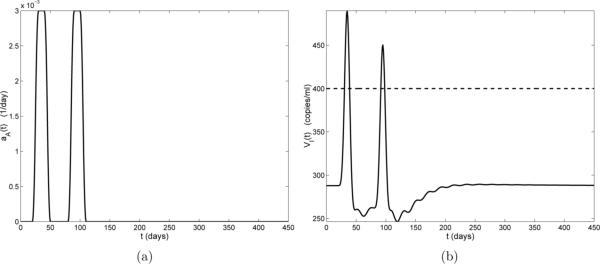
We next investigate the effect of sequential non-HIV infections by simulating two such back-to-back infections. The first infection occurs from days 20 through 50 and stays at its peak value (0.003 day−1) from days 30 through 40, while the second infection occurs from days 80 through 110 and stays at its peak value (0.003 day−1) from days 90 through 100 (Fig. 6(a)). As seen in Fig. 6(b), the first infection leads to a viral blip at exactly the same time as that in Fig. 4 and the second infection leads to a viral blip (starting at day 95) with the same duration as the first, but with a smaller amplitude.
Figure 6.
(a) Activation rate by non-HIV antigens aA(t). The duration of each infection is 30 days, with the first beginning on day 20 and the second on day 80; (b) Viral load VI(t) (solid line) and censor data level (horizontal dashed line).
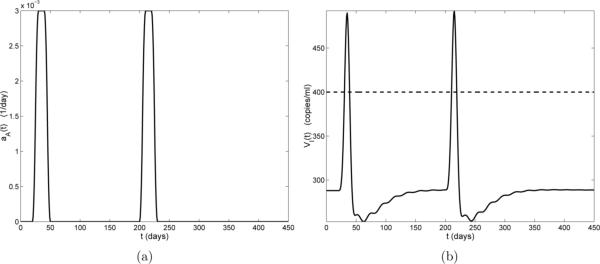
To investigate whether the short time interval between these two infections leads to the suppressed amplitude of the second viral blip, we also considered a case where the first infection is the same as that in Fig. 6 (days 20 through 50) but the second infection occurs much later (days 200 through 230). The simulation results are illustrated in Fig. 7, which indicates that the amplitude of the second viral blip now approximately the same as the first viral blip.
Figure 7.
(a) Activation rate by non-HIV antigens aA(t). The duration of each infection is 30 days, with the first beginning on day 20 and the second on day 200; (b) Viral load VI(t) (solid line) and censor data level (horizontal dashed line).
Based on these examples, we see that the frequency of non-HIV infections affects the frequency of the viral blips and that the time interval between the two infections can affect the amplitude of the second viral blip. In particular, the shorter the time interval between two infections, the smaller the amplitude of the second viral blip. This suggests that it is possible that there may be only one viral blip detected if the time interval between the two infections is short enough.
To further investigate the dynamics of two sequential infections, we plot the other model compartments in Fig. 8, where we observe that the E1 and E2 compartments are still below their equilibrium values when the second infection occurs. This may explain the slight increase in amplitude of the second viral blip. In the case of the more closely-spaced second infection of Fig. 6(a), the start of which is indicated with the dotted vertical line in Fig. 8, we can see that E1 and E2 are above their equilibrium levels. This may explain the decreased amplitude of the second viral blip in Fig. 6(b).
Figure 8.
Model dynamics with ε1 = 0.7, ε2 = 0, and the values of all the other parameters as specified in Table 2. Activation rate by a non-HIV antigen aA(t) is as depicted in Fig. 7(a). Vertical dashed lines indicate the start and stop times of the non-HIV infections for this example. The vertical dotted line indicates the start time (80 days) of the second infection in Fig. 6.
CD4+ help during transient viremia
In model (2.1), the differentiation of E1 cells to E2 memory cells occurs through the term , which is dependent on the help of activated CD4+ cells (T1 and ). In the case that T1 and are zero, there is no differentiation of the effector E1 cells into memory E2 cells. On the other hand, in the limit of large T1 + , the maximum rate of differentiation γEE1 is attained. In this section we explore what effect the CD4+ help has on the CD8+ immune response and we do so in the context of transient viremia induced by a non-HIV infection aA(t). We use the parameter Kγ to modify the effects of the CD4+ help. The case of Kγ = 0 simulates a condition where CD4+ help is not required for differentiation to CD8+ memory, while the case of Kγ very large simulates a condition where differentiation to CD8+ memory is impaired due to lack of CD4+ help. Thus, we use the states of locally a.s. “healthy” infected equilibria, corresponding to ε1 = 0.7, ε2 = 0, aA = 0, various values of Kγ, and the values of all other parameters as specified in Table 2, as the initial conditions for simulations in which we allow the parameter aA to be a function of time t. As we drive the system (2.1) with the non-HIV infection aA(t) we monitor the states of the system.
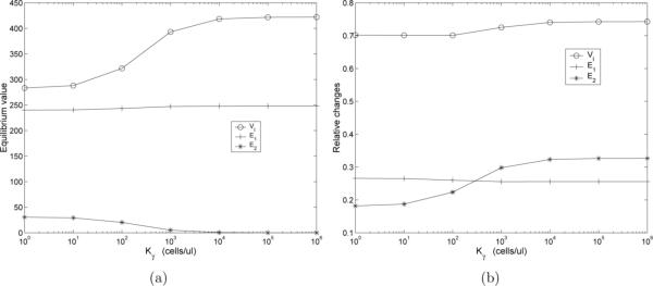
In Fig. 9(a) we plot the “healthy” infected (EQ2) equilibrium values of the VI, E1, and E2 compartments as a function of Kγ. As expected, as Kγ increases, corresponding to increasing impairment of CD8+ differentiation to memory, the equilibrium value of the E2 compartment decreases. However, the overall effect on E1 is negligible with only a slight rise as Kγ increases. Despite the fact that E1 stays relatively constant, we see that, as Kγ increases, the equilibrium value of the viral load increases until reaching a plateau value at Kγ ≈ 1 × 10⁵ cells/μl-blood. Thus, even though the number of effector cells, which directly participate in the removal of infected T-cells, does not decrease as the CD8+ differentiation to memory is impaired, the overall viral load increases.
Figure 9.
(a) The effect of Kγ on the “healthy” infected (EQ2) values of the VI (circles), E1 (crosses), and E2 (asterisks) compartments. Equilibrium values correspond to the case ε1 = 0.7, ε2 = 0, aA = 0, and the values of all other parameters as specified in Table 5; (b) Relative change of VI (circles), E1 (crosses), and E2 (asterisks) compartments as a function of Kγ.
In Fig. 9(b) we plot the relative changes of the various compartments as a function of Kγ. Relative change is defined as (peak value minus initial value)/(initial value). In this figure we can see that, as Kγ increases the relative change of the peak viral load increases. The relative change of the E2 memory compartment also increases (Fig. 9(b)), but the infected equilibrium value was quite small to begin with (Fig. 9(a)). The relative change in the effector E1 compartment decreases as Kγ increases. The results of this analysis demonstrates that in our model, impaired differentiation to CD8+ memory results in a degraded “healthy” equilibrium and leads to a larger viral blip following a secondary infection.
5 Application of the Model to Clinical Data
The data for our investigations come from Massachusetts General Hospital (MGH), where all the patients enrolled in the study are symptomatic with acute or early HIV-infection (for more detailed information of these data, the interested reader is referred to [3, 23, 29]). In summary, nearly all subjects in the study undergo combination therapy and many have at least one treatment interruption. The available clinical data include total CD4+ T-cell count and total RNA copies, where for model (2.1) the total CD4+ T-cell counts are represented by and total RNA copies are represented by z̄2(t; q) = VI(t; q) + VNI(t; q). If the measurements of RNA copies are below the limit of quantification for the assay used (400 copies/ml-plasma for a standard assay and 50 copies/ml-plasma for an ultra-sensitive assay), then the observed viral load value is censored to be at its detection limit; that is, in these cases the observed values do not represent the true data values anymore. Furthermore, observations of viral load and CD4+ may not be at the same time points and the observation times and intervals vary substantially among patients. So, in general, for patient number j we have CD4+ T-cell data pairs , and potentially different time point viral RNA data pairs . Hence, the clinical data for carrying out the inverse problem involves partial observations, measurements from combined compartments, and highly censored viral load measurements.
We use the clinical data in two ways: for estimating parameter values and for testing the predictive capability of the model. For the (new) model (2.1) presented here most parameters can not be determined a priori and therefore must be estimated from data. In Section 5.1 we show how we use the clinical data to formulate an inverse problem to obtain parameter estimates for each patient. Using the collective parameter estimates for all the patients and knowledge of model sensitivities we then fix some model parameters and initial conditions at the population averages across these patients and re-estimate the remaining free parameters for each individual.
In Section 5.2 we use the same values for the fixed model parameters and initial conditions as obtained in Section 5.1 and estimate the remaining free parameters using only half of the longitudinal data for each patient. Using the parameters thus obtained, we use the model to predict the time course of the disease during the time period corresponding to the second half of the longitudinal data and compare these model predictions to the actual data.
As one might expect, if a patient does not have a sufficient number of observations or does not undergo a therapy interruption during the observation period used to fit the model, then it is difficult to obtain accurate estimations of the dynamically dependent parameters. We are interested in using this model to predict later disease progression involving both therapy and treatment interruption (see Section 5.2). Hence, for our purposes we focus on 14 patients with sufficient data and at least one on/off treatment schedule in the first half of their longitudinal data. Note that for each of these patients, is not substantially different than .
5.1 Fitting the Model/Parameter Estimation
To obtain patient specific-parameter estimates for the model, we use individual patient data and carry out an inverse problem. The technique we use in this paper is adapted from the one in [3], where the authors developed a statistically-based censored data method (an expectation maximization algorithm) combined with an ordinary nonlinear least-squares technique. We note that the variance in CD4 measurements and the variance in viral load measurements are likely to be different due to assay differences. Hence, in this paper we use the expectation maximization algorithm based on Maximum Likelihood Estimation for which, under normality assumptions on the errors, results in a weighted least-squares technique (see [32]) with solution given by
| (5.1) |
for the log10-transformed system of model (2.1) for patient j, where and , and . As noted in [3], by using a log-transformed system one can resolve a problem of states becoming unrealistically negative due to round-off error: nonnegative solutions of this model should stay so throughout numerical simulation. This approach also enables efficient handling of unrealistic cases where states get infinitesimally small during integration due to parameters selected by optimization algorithms. From a statistical point of view, log transformation is a standard technique to render the observations more nearly normally distributed, which also supports use of the weighted least squares criterion as an equivalent to maximum likelihood estimation.
The expectation maximization (EM) algorithm is outlined below. To simplify the notation, we drop the patient index j in this algorithm description. The following notation will be used in the algorithm: the relevant censoring point at time ti is represented by Li and χi is the indicator function for the set , ϕ denotes the standard normal probability density function and Φ is the corresponding cumulative distribution function. For each patient, we carried out the following parameter estimation algorithm:
- (Step 1) Create adjusted data ỹi by replacing censored values by Li/2, and use ordinary least squares to estimate q̂(0) using both CD4+ data and adjusted viral RNA data ỹi (which now includes replaced censored values).
Obtain an initial estimate for and from
respectively. Set k = 0. - (Step 2) Define and . Update the data and residuals by
- (Step 3) Update the estimate of q to q̃(k+1) by performing the weighted least squares minimization in the parameters q
and computing
If relative changes in q̂, and are small, terminate. Otherwise set k = k + 1 and then go to Step 2.
Although the EM algorithm may seem unnecessarily complicated, it should be noted that previous attempts to fit censored clinical data without the EM algorithm produced extremely poor results. For more details about the EM algorithm and how to carry it out, interested readers are referred to [3, 13, 25].
As noted previously, model (2.1) modifies and extends the model in [3] to incorporate important features of HIV pathogenesis. However, the cost of this more biologically detailed model is a larger set of free parameters: 31 model parameters and 8 initial conditions. Hence, we seek to reduce the number of free parameters. We first estimate all 39 parameters for each of the 14 patients by applying the EM algorithm to the full longitudinal data set, where the total number of data points (sum of number of CD4+ data points and number of viral load data points) varies from 71 to 273. We then fix 23 parameters at the population averages across these patients, and re-estimate the remaining 16 parameters for each patient by applying the EM algorithm to the full longitudinal data set. Note that there exists biological variation in all parameters across the patients, and there also exist high correlations among some of these parameters such as the RNA copies produced per infected cells NT and the virus natural death rate c. We also observe that sensitivity with respect to some of these parameters may be highly time-dependent. For example, the dynamics of the model is much more sensitive to the treatment efficacies ε1 and ε2 in the treatment periods than it is in the off-treatment periods. All of these considerations make it difficult to choose a priori which parameters can be fixed. In this paper, we empirically chose some parameters (such as the saturation parameters) to which the model appears to be relatively insensitive to take as fixed. Table 5 specifies all the fixed parameters (19 model parameters and 4 initial conditions) and their corresponding values.
Table 5.
Average model parameter values (19) and initial conditions (4) used in model fitting with half and full longitudinal data set.
| γ t | 3.792e-04 | d 2 | 3.096e-03 | f | 5.068e-01 |
| k 2 | 2.005e-09 | δ | 2.095e-01 | m | 1.127e-03 |
| c | 5.818e+00 | λ e | 9.930e-04 | bE 1 | 3.885e-02 |
| Kb 1 | 2.488e-02 | dE | 6.278e-02 | Kd | 1.200e-01 |
| δ e 1 | 5.967e-02 | Kb 2 | 8.697e+01 | γ e | 5.154e-04 |
| Kγ | 1.357e+00 | KV | 1.479e+01 | δ E 2 | 1.450e-03 |
| Ks | 2.789e+04 | 7.521e-03 | 3.571e+03 | ||
| 6.821e-02 | 6.909e-01 |
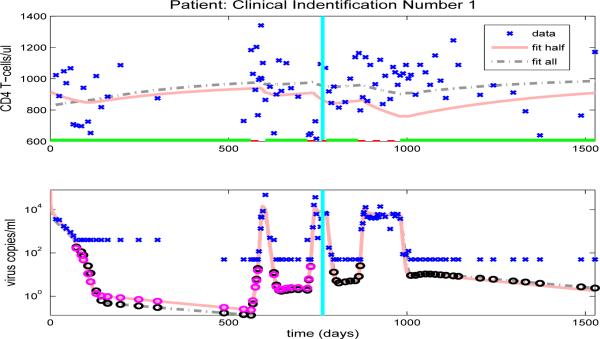
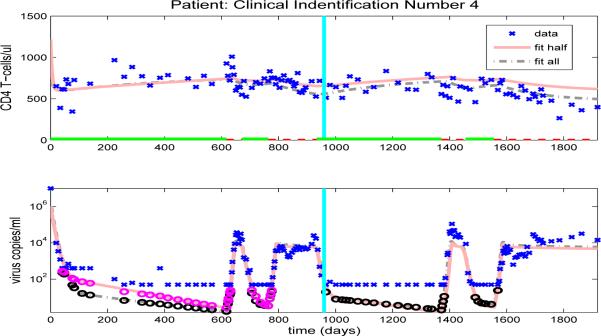
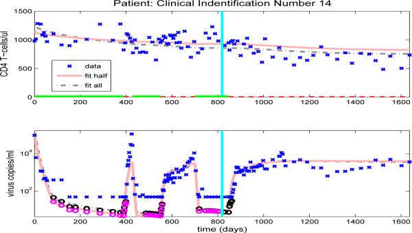
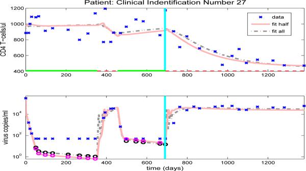
After we estimate the reduced set of 16 free parameters (using the full set of data, in an inverse problem), we simulate the CD4+ T-cell and viral load trajectories over the full time span of the patient's observations by using the parameter values obtained and compare to the experimental data. Figures 10-13, and Figures 14-23 in the Appendix illustrate model fits (dash-dot lines) for all 14 patients. These figures reveal that the fits to CD4+ T-cells and the fits to viral load are reasonable when using the full data set to estimate the parameter values, as illustrated in Figure 10 for patient 1.
Figure 10.
Clinical data (‘x’) for CD4 T-cells (upper graph) and viral load (lower graph). Also included are the model results with parameters estimated from full data (dash-dot line) or half longitudinal data (solid line). Dark and gray circles denote the predicted censored data values for the full and half longitudinal data, respectively. The vertical line in the middle of the graph delineates between the two halves of the longitudinal data. A solid line along the x-axis in the upper figure indicates periods when the patient is on HAART treatment, while a dashed line indicates off-treatment periods.
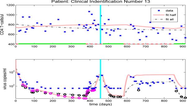
Figure 13.
Clinical data (‘x’) for CD4 T-cells (upper graph) and viral load (lower graph). Also included are the model results with parameters estimated from full data (dash-dot line) or half longitudinal data (solid line). Dark and gray circles denote the predicted censored data values for the full and half longitudinal data, respectively. The vertical line in the middle of the graph delineates between the two halves of the longitudinal data. A solid line along the x-axis in the upper figure indicates periods when the patient is on HAART treatment, while a dashed line indicates off-treatment periods.
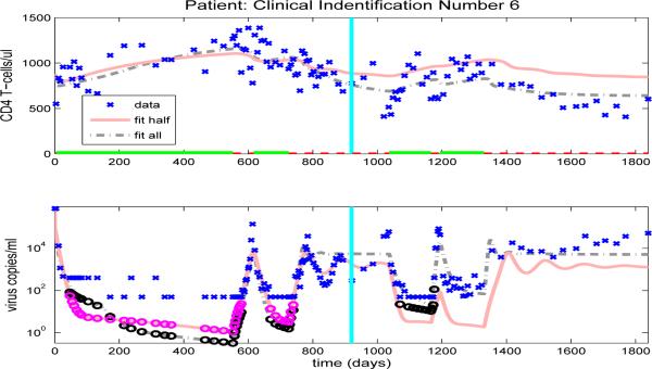
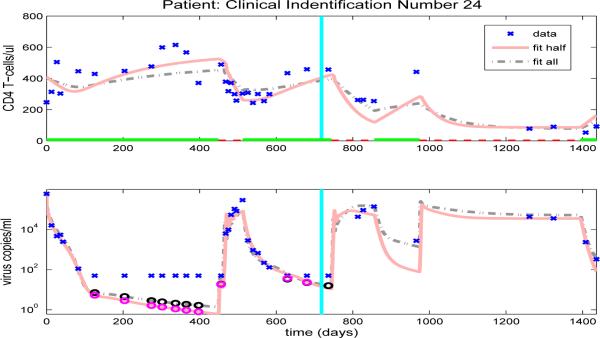
Figure 14.
CD4 T-cells (upper graph) and viral load (lower graph).
Figure 23.
CD4 T-cells (upper graph) and viral load (lower graph).
5.2 Predictive Capability of the Model
When proposing a new model, a necessary but often difficult requirement is validation of the model with clinical data. One way to do this is to use the first part of the available longitudinal data for a given patient to estimate patient specific parameters. One then uses these parameters in model simulations to accurately predict the subsequent progression of the disease as represented in the remainder of the longitudinal data for that patient. In this section, we retain the same values for the 23 fixed parameters as above (Table 5) and estimate the remaining 16 free parameters using only half of the longitudinal data, where the total number of data points varies from 42 to 154. Using the parameters thus obtained, we use model (2.1) to predict the time course of the CD4+ T-cell count and viral load corresponding to the second half of the longitudinal data and compare these model predictions to the actual data.
Figures 10-13, and Figures 14-23 in the Appendix illustrate model predictions (solid lines) for all 14 patients. These figures reveal that both the fits to CD4+ T-cells and the fits to viral load are reasonable when using half data to estimate the free parameter values, even with multiple on/off-treatments, as illustrated in Figure 11 for patient 4.
Figure 11.
Clinical data (‘x’) for CD4 T-cells (upper graph) and viral load (lower graph). Also included are the model results with parameters estimated from full data (dash-dot line) or half longitudinal data (solid line). Dark and gray circles denote the predicted censored data values for the full and half longitudinal data, respectively. The vertical line in the middle of the graph delineates between the two halves of the longitudinal data. A solid line along the x-axis in the upper figure indicates periods when the patient is on HAART treatment, while a dashed line indicates off-treatment periods.
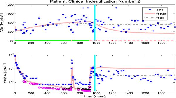
However, there is under- or over-prediction for some patients when using parameters estimated from the half data set. For example, model fits obtained by using half time series data for patient 2 are shown in Fig. 12 (solid line), where it can be seen that by using parameters estimated from the first half data set, the predicted values for viral load data are higher and the predicted values for CD4+ T-cell are lower than the observed data values, even though there are two off-treatment periods in the first half of the data set. This discrepancy may be due to the fact that both off-treatment periods are short and, therefore, provide very little information about the off-treatment behavior. Note that, for this patient, the values of most observations of viral loads in the off-treatment periods during the first half data set are higher than those observed in the second half data set and this makes it difficult to correctly predict future off-treatment trends. Hence, it is not just the number of off-treatment periods in the first half data set but also the length of each off-treatment period and the number of observations in these periods that determines the accuracy of the predictions of off-treatment viral load levels.
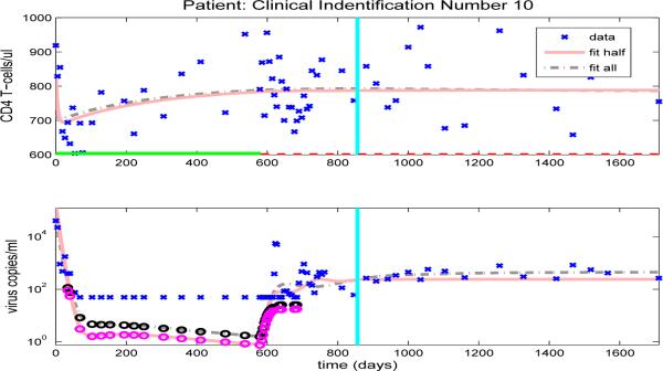
Figure 12.
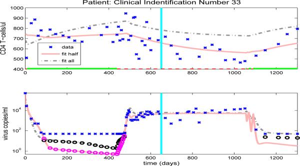
Clinical data (‘x’) for CD4 T-cells (upper graph) and viral load (lower graph). Also included are the model results with parameters estimated from full data (dash-dot line) or half longitudinal data (solid line). Dark and gray circles denote the predicted censored data values for the full and half longitudinal data, respectively. The vertical line in the middle of the graph delineates between the two halves of the longitudinal data. A solid line along the x-axis in the upper figure indicates periods when the patient is on HAART treatment, while a dashed line indicates off-treatment periods.
In contrast, Figure 13 compares the model fit and prediction obtained by using the half data set to clinical data for patient 10. Even though there is only one off-treatment period in the first half data set, the period is longer with a richer data set and the half data predictions of both CD4+ T-cell and viral load agree quite well in the second half data set. Hence, the results demonstrated in Figures 12 and 13 suggest that in order to have accurate predictive capability we need to obtain a sufficient number of representative data points in the time period providing the information about the dynamics (the time period used to estimate parameters).
Finally, we note that the model developed and tested here retains the predictive capabilities present in the earlier model of [3] in that the ability to predict subsequent data after fitting the model with half of the data is at least as good as that exhibited in [3] for the various patients in our data sets. In addition, the added complexity of creating a more accurate description of the underlying biological processes is greatly offset by fixing many of the parameter values at their population averages. While by no means a definitive validation of the model, these results suggest that, given data on a new patient, it may be possible to fit this new data with the smaller subset of 16 free parameters (and fixed parameters in Table 5) and that, using the parameter values thus obtained, we can reasonably predict subsequent disease progression in the near future.
6 Multiple Equilibria and Clinical Patients
One of the requirements of our model is that it can admit multiple locally a.s. off-treatment equilibria. The existence of multiple equilibria is necessary if we seek to use therapeutic intervention to move a patient from an unhealthy (very high viral load) to a healthier equilibrium (lower viral load). In Section 3 we demonstrated the existence of multiple locally a.s. off-treatment equilibria for model (2.1) with a particular set of model parameters. As demonstrated in Section 3, the number of equilibrium states is dependent on the specific values of the parameters. In this section, we present results using the parameter estimates obtained from the full set of patient clinical data (Section 5.1) to investigate the number of locally a.s steady states available to each patient.
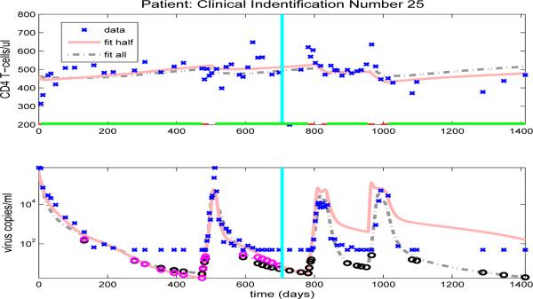
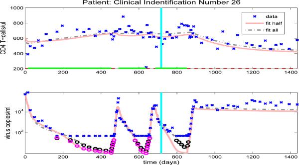
Using parameter estimates obtained in Section 5.1 we find that all patients have only one off-treatment, locally a.s. infected equilibrium state, although the viral loads of the infected equilibrium states vary from approximately 450 to 51600 copies/ml-plasma, depending upon the patient. We also find that the majority of patients have no locally a.s. uninfected equilibrium state. However, the parameter sets for two patients (25 and 26) did admit a locally a.s. uninfected equilibrium state. At this point we do not have enough information to know whether the existence of locally a.s. uninfected equilibria for these two patients is clinically meaningful.
We note that the existence of an uninfected equilibrium state or a second infected equilibrium state can be sensitive to small collective changes in the parameter values, even though these values may still give reasonable fits to the data. However, we generally find that the majority of patients have neither an uninfected equilibrium state nor a second infected equilibrium state. This suggests that treatment to move from a high viral load equilibrium state to an equilibrium state with a lower (or zero) viral load, as proposed in [1, 2], is not possible for these patients.
7 Conclusion and Remarks
We present a system of ordinary differential equations to describe the pathogenesis of HIV infection. This model provides a more accurate biological description of the underlying infection and immune response than a previous model [3], including a compartment for CD4+ memory cells that serve as a major reservoir of latently infected cells, a critical role for T-helper cells in the generation of CD8 memory cells capable of efficient recall response, and stimulation by antigens other than HIV. A stability analysis illustrates the capability of this model for admitting multiple locally asymptotically stable (locally a.s.) off-treatment equilibria. The existence of these off-treatment equilibria allow for the possibility of treatment strategies that would shift patients from higher viral load equilibrium states to lower viral load equilibrium states.
We show that this more biologically-detailed model can exhibit the phenomenon of “viral blips” or transient viremia experienced by some patients on therapy with viral load levels suppressed below the detection limit, something not possible with the previous model. We also use this more biologically-detailed model to explore the effect of CD4+ T-cell help on the CD8+ T-cell immune response in the context of transient viremia induced by a non-HIV infection. The results of this analysis demonstrates that in our model, impaired differentiation to CD8+ memory results in an infected equilibrium exhibiting a higher viral load and leads to a larger viral blip following a secondary infection.
Application of this model to censored clinical data to obtain parameter estimates demonstrates that using a reduced set of 16 free parameters, obtained by fixing 23 parameters at their population averages, the model provides good fits to the patient data. Furthermore, we demonstrate the strong predictive capability of the model for longer term behavior by using estimates of the 16 free parameters obtained from half of the longitudinal data to compare model predictions to the second half of the clinical data. These results suggest that it may be possible to fit new patient data with the smaller subset of 16 free parameters (and the fixed parameters in Table 5) and that, using the parameter values thus obtained, we may be able to predict subsequent disease progression in the near future. We further show that parameter values obtained for most clinical patients do not admit multiple locally a.s off-treatment equilibria in the corresponding model. This suggests that therapy regimes designed to move the patient from a high viral load equilibrium state to an equilibrium state with a lower (or zero) viral load may not be possible for these patients.
One of the challenges in our clinical data fitting is that we do not have sufficiently rich data sets to fit all the model parameters and initial conditions. Due to the high correlations between the model parameters, biological variations in all parameters across population and the sensitivity with respect to parameters varying over time (especially during the transition time between the off-treatment period and on-treatment period), we empirically chose some parameters in this paper to be fixed. Even though the simulation results indicate reasonable fits to data of each of the patients, we need to develop a scientific methodology to deal with this situation in order to obtain more reliable parameter values to be fixed a priori and thereby sharpen our estimation results. As outlined above we reduced the number of parameters to be estimated by fixing some of the parameters at population averages. In clinical cases where large, long term individual patient longitudinal data sets are not available as in our study here, one could use population averages accrued in prior patient trials to reduce the number of free parameters. Another possible method to reduce the dimension of parameter space and the associated high correlation between these parameters is principal component analysis, which is currently under investigation.
The clinical data fitting results in Section 5 indicate that if one does not have a sufficient number of observations during the periods where the dynamics are changing, then it is difficult to obtain parameter estimates useful in predicting corresponding future trends in disease progression. Hence, the goodness of fit results are affected by not only the number of observations but also the sampling times for data collection. This general principle was also observed and explained conceptually in [6] where the general “information content” in data and its relation to sensitivity is explored. These considerations suggest that parameter sensitivity with respect to data is important in experimental design, assisting in reducing effort and resources required to collect necessary data. One potential approach for this is the generalized sensitivity function methodology as proposed in [38] and explored in [5, 7]. This approach combines the sensitivities of model output with respect to model parameters with the sensitivities of parameters estimates with respect to changes in model outputs. Obtaining results using this methodology is challenging even for simple examples and our initial efforts have not yet proved fruitful for our complex HIV models which feature high correlations between some parameters and dynamics that dramatically change during the transition time between off-treatment and on-treatment. Hence, one of our future efforts involves development of a methodology to determine improved sampling times for data collection. We are optimistic that ideas contained in principal component analysis and generalized sensitivity functions can be combined to provide new guidance in this regard.
Figure 15.
CD4 T-cells (upper graph) and viral load (lower graph).
Figure 16.
CD4 T-cells (upper graph) and viral load (lower graph).
Figure 17.
CD4 T-cells (upper graph) and viral load (lower graph).
Figure 18.
CD4 T-cells (upper graph) and viral load (lower graph).
Figure 19.
CD4 T-cells (upper graph) and viral load (lower graph).
Figure 20.
CD4 T-cells (upper graph) and viral load (lower graph).
Figure 21.
CD4 T-cells (upper graph) and viral load (lower graph).
Figure 22.
CD4 T-cells (upper graph) and viral load (lower graph).
Acknowledgements
This research was supported in part by the National Institute of Allergy and Infectious Disease under grant 9R01AI071915−05, and in part by the U.S. Air Force Office of Scientific Research under grant AFOSR-FA9550−04−1−0220. The authors are grateful to Alan Perelson for discussions that stimulated our interests in the viral blips occurring in HIV clinical data.
Appendix: Section 5 Results for Other Patients
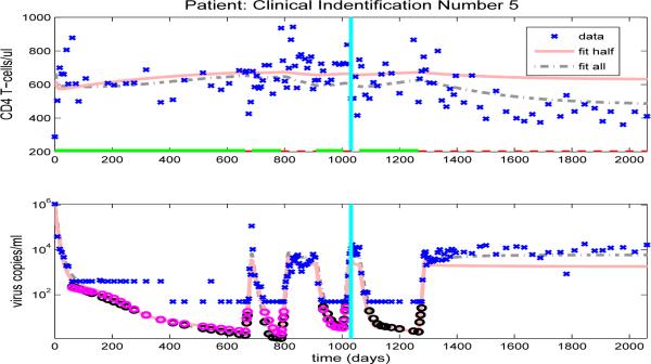
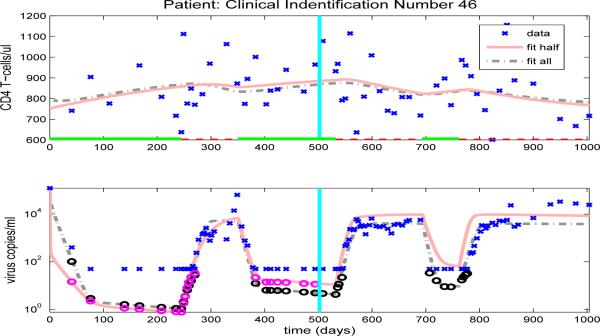
The model fits for the remaining clinical patients are shown in Figures 14-23. As in previous figures, clinical data (‘x’) for CD4 T-cells and viral load are shown in the upper and lower graphs, respectively. Also included in the figures are the model results with parameters estimated from full data (dash-dot line) or half longitudinal data (solid line). Dark and gray circles denote the predicted censored data values for the full and half longitudinal data, respectively. The vertical line in the middle of the graph delineates between the two halves of the longitudinal data. A solid line along the x-axis in the upper figure indicates periods when the patient is on HAART treatment, while a dashed line indicates off-treatment periods.
References
- 1.Adams BM, Banks HT, Davidian M, Kwon H, Tran HT, Wynne SN, Rosenberg ES. HIV dynamics: modeling, data analysis, and optimal treatment protocols. J. Computational and Applied Mathematics. 2005;184:10–49. [Google Scholar]
- 2.Adams BM, Banks HT, Tran HT, Kwon H. Dynamic multidrug therapies for HIV: optimal and STI control approaches. Mathematical Biosciences and Engineering. 2004;1:223–241. doi: 10.3934/mbe.2004.1.223. [DOI] [PubMed] [Google Scholar]
- 3.Adams BM, Banks HT, Davidian M, Rosenberg ES. Model fitting and prediction with HIV treatment interruption data. Bulletin of Mathematical Biology. 2007;69:563–584. doi: 10.1007/s11538-006-9140-6. CRSC-TR05−40, NCSU, October, 2005. [DOI] [PubMed] [Google Scholar]
- 4.Altfeld M, Rosenberg ES. The role of CD4 T helper cells in the cytotoxic T lymphocyte response to HIV-1. Current Opinion in Immunology. 2000;12:375–380. doi: 10.1016/s0952-7915(00)00103-5. [DOI] [PubMed] [Google Scholar]
- 5.Bai P, Banks HT, Dediu S, Govan AY, Last M, Loyd A, Nguyen HK, Olufsen MS, Rempala G, Slenning BD. Stochastic and deterministic models for agricultural production networks. Mathematical Biosciences and Engineering. 2007;4:373–402. doi: 10.3934/mbe.2007.4.373. CRSC-TR07−06, NCSU, February, 2007. [DOI] [PubMed] [Google Scholar]
- 6.Banks HT, Ernstberger SL, Grove SL. Standard errors and confidence intervals in inverse problems: Sensitivity and associated pitfalls. J. Inverse and Ill-posed Problems. 2006;15:1–18. CRSC-TR06−10, NCSU, March, 2006. [Google Scholar]
- 7.Batzel JJ, Kappel F, Schneditz D, Tran HT. Cardiovascular and Respiratory Systems: Modeling, Analysis and Control. SIAM; Philadelphia: 2006. SIAM Frontiers in Applied Math. [Google Scholar]
- 8.Bevan MJ. Helping the CD8+ T-cell response. Nature Reviews. 2004;4:595–602. doi: 10.1038/nri1413. [DOI] [PubMed] [Google Scholar]
- 9.Blankson JN, Persaud D, Siliciano RR. The challenge of viral reservoirs in HIV-1 infection. Annual Review of Medicine. 2002;53:557–593. doi: 10.1146/annurev.med.53.082901.104024. [DOI] [PubMed] [Google Scholar]
- 10.Bonhoeffer S, Rembiszewski M, Ortiz GM, Nixon DF. Risks and benefits of structured antiretroviral drug therapy interruptions in HIV-1 infection. AIDS. 2000;14:2313–2322. doi: 10.1097/00002030-200010200-00012. [DOI] [PubMed] [Google Scholar]
- 11.Brenchley JM, Hill BJ, Ambrozak DR, Price DA, Guenaga FJ, Casazza JP, Kuruppu J, Yazdani J, Migueles SA, Connors M, Roederer M, Douek DC, Koup RA. T-cell subsets that harbor human immunodificiency virus (HIV) in vivo: implications for HIV pathogenesis. J. of Virology. 2004;78:1160–1168. doi: 10.1128/JVI.78.3.1160-1168.2004. [DOI] [PMC free article] [PubMed] [Google Scholar]
- 12.Callaway DS, Perelson AS. HIV-1 infection and low steady state viral loads. Bulletin of Mathematical Biology. 2001;64:29–64. doi: 10.1006/bulm.2001.0266. [DOI] [PubMed] [Google Scholar]
- 13.Dempster AP, Laird NM, Rubin DB. Maximum likelihood from incomplete data via the EM algorithm. J. Roy. Stat. Soc., Ser. B. 1977;39:1–38. [Google Scholar]
- 14.Douek DC, Brenchley JM, Betts MR, Ambrozak DR, Hill BJ, Okamoto Y, Casazza JP, Kuruppu J, Kuntsman K, Wolinsky S, Grossman Z, Dybul M, Oxenius A, Price DA, Connors M, Koup RA. HIV preferentially infects HIV-specific CD4(+) T cells. Nature. 2002;417:95–98. doi: 10.1038/417095a. [DOI] [PubMed] [Google Scholar]
- 15.Chun T-W, Carruth L, Finzi D, Shen XF, DiGiuseppe JA, Taylor H, Hermankov M, Chadwick K, Margolick J, Quinn TC, Kuo YH, Brookmeyer R, Zeiger MA, BarditchCrovo P, Siliciano RF. Quantification of latent tissue reserviors and total body viral load in HIV-1 infection. Nature. 1997;387:183–188. doi: 10.1038/387183a0. [DOI] [PubMed] [Google Scholar]
- 16.Di Mascio M, Markowitz M, Louie M, Hogan C, Hurly A, Ho DD, Perelson AS. Viral blip dynamics during highly active antiretroviral therapy. J. of Virology. 2003;77:12165–12172. doi: 10.1128/JVI.77.22.12165-12172.2003. [DOI] [PMC free article] [PubMed] [Google Scholar]
- 17.Dixit NM, Perelson AS. Complex patterns of viral load decay under antiretroviral therapy: influence of pharmacokineticsand intracellular delay. J. of Theoretical Biology. 2004;226:95–109. doi: 10.1016/j.jtbi.2003.09.002. [DOI] [PubMed] [Google Scholar]
- 18.Finzi D, Hermankova M, Pierson T, Carruth LM, Buck C, Chaisson RE, Quinn TC, Chadwick K, Margolick J, Brookmeyer R, Gallant J, Markowitz M, Ho DD, Richman DD, Siliciano RF. Identification of a reservoir for HIV-1 in patients on highly active antiretroviral therapy. Science. 1997;278:1295–1300. doi: 10.1126/science.278.5341.1295. [DOI] [PubMed] [Google Scholar]
- 19.Haase AT. Population biology of HIV-1 infection: Viral and CD4(+) T cell demographics and dynamics in lymphatic tissues. Annual Review of Immunology. 1999;17:625–656. doi: 10.1146/annurev.immunol.17.1.625. [DOI] [PubMed] [Google Scholar]
- 20.Ho DD, Neumann AU, Perelson AS, Chen W, Leonard JM, Markowitz M. Rapid turnoverof plasma virions and CD4 lymphocytes in HIV-1 infection. Nature. 1995;373:123–126. doi: 10.1038/373123a0. [DOI] [PubMed] [Google Scholar]
- 21.Janssen EM, Lemmens EE, Wolfe T, Christen U, Von Herrath MG, Schoenberger SP. CD4+ T-cells are required for secondary expansion and memory in CD8+ T lymphocytes. Nature. 2003;421:852–856. doi: 10.1038/nature01441. [DOI] [PubMed] [Google Scholar]
- 22.Jones LE, Perelson AS. Opportunistic infection as a cause of transient viremia in chronically infected HIV patients under treatment with HAART. Bulletin of Mathematical Biology. 2005;67:1227–1251. doi: 10.1016/j.bulm.2005.01.006. [DOI] [PubMed] [Google Scholar]
- 23.Kassutto S, Maghsoudi K, Johnston M, Robbins G, Burgett N, Sax P, Cohen D, Pae E, Davis B, Zachary K, Basgoz N, D'agata EMC, DeGruttola V, Walker B, Rosenberg E. Longitudinal analysis of clinical markers following antiretroviral therapy initiated during acute or early HIV-1 infection. Clinical Infectious Disease. 2006;42:1024–1031. doi: 10.1086/500410. [DOI] [PubMed] [Google Scholar]
- 24.McCune JM. The dynamics of CD4+ T-cell depletion in HIV disease. Nature. 2001;410:974–979. doi: 10.1038/35073648. [DOI] [PubMed] [Google Scholar]
- 25.McLachlan GJ, Krishnan T. The EM Algorithm and Extensions. John Wiley; New York: 1997. [Google Scholar]
- 26.Nowak MA, Bangham CRM. Population dynamics of immune responses to persistent viruses. Science. 1996;272:74–79. doi: 10.1126/science.272.5258.74. [DOI] [PubMed] [Google Scholar]
- 27.Perelson AS, Essunger P, Cao YZ, Vesanen M, Hurley A, Saksela K, Markowitz M, Ho DD. Decay characteristics of HIV-1-infected compartments during combination therapy. Nature. 1997;387:187–191. doi: 10.1038/387188a0. [DOI] [PubMed] [Google Scholar]
- 28.Perelson AS, Nelson PW. Mathematical analysis of HIV-1 dynamics in vivo. SIAM Review. 1999;41:3–44. [Google Scholar]
- 29.Rosenberg ES, Altfield M, Poon SH, Phillips MN, Wilkes B, Eldridge RL, Robbins GK, D'Aquila RD, Goulder PJR, Walker BD. Immune control of HIV-1 after early treatment of acute infection. Nature. 2000;407:523–526. doi: 10.1038/35035103. [DOI] [PubMed] [Google Scholar]
- 30.Rowland-Jones SL, Dong T, Fowke KR, Kimani J, Krausa P, Newell H, Blanchard T, Ariyoshi K, Oyugi J, Ngugi E, Bwayo J, MacDonald KS, McMichael AJ, Plummer FA. Cytotoxic T-cell responses to multiple conserved HIV epitopes in HIV-resistant prostitute in Nairobi. J. of Clinical Investigation. 1998;102:1758–1765. doi: 10.1172/JCI4314. [DOI] [PMC free article] [PubMed] [Google Scholar]
- 31.Pinto LA, Sullivan J, Berzofsky JA, Clerici M, Kessler HA, Landay AL, Shearer GM. ENV-specific cytotoxic T lymphocyte responses in HIV seronegative health care workers occupationally exposed to HIV-contaminated body fluids. J. of Clinical Investigation. 1995;96:867–876. doi: 10.1172/JCI118133. [DOI] [PMC free article] [PubMed] [Google Scholar]
- 32.Seber GAF, Wild CJ. Nonlinear Regression. John Wiley & Sons, Inc.; New York: 1989. [Google Scholar]
- 33.Seder RA, Ahmed R. Similarities and differences in CD4+ and CD8+ effector and memory T-cell generation. Nature Immunology. 2003;4:835–842. doi: 10.1038/ni969. [DOI] [PubMed] [Google Scholar]
- 34.Shedlock DJ, Shen H. Requirement for CD4 T-cell help in generating functional CD8 T-cell memory. Science. 2003;300:337–339. doi: 10.1126/science.1082305. [DOI] [PubMed] [Google Scholar]
- 35.Siliciano JD, Kajdas J, Finzi D, Quinn TC, Chadwick K, Margolick JB, Kovacs C, Gange SJ, Siliciano RF. Long-term follow-up studies confirmed the stability of the latent reservior for HIV-1 in resting CD4+ T-cells. Nature Medicine. 2003;9:727–728. doi: 10.1038/nm880. [DOI] [PubMed] [Google Scholar]
- 36.Sprent J, Surh CD. T-cell memory. Annual Rev. Immunol. 2002;20:551–579. doi: 10.1146/annurev.immunol.20.100101.151926. [DOI] [PubMed] [Google Scholar]
- 37.Streeck H, Jessen H, Alter G, Teigen N, Waring MT, Jessen A, Stahmer I, van Lunzen J, Ichterfeld M, Gao XJ, Allen TM, Carrington M, Walker BD, Rockstroh JK, Altfeld M. Immunological and virological impact of highly active antiretroviral therapy initiated during acute HIV-1 infection. J. of Infectious Diseases. 2006;194:734–739. doi: 10.1086/503811. [DOI] [PubMed] [Google Scholar]
- 38.Thomaseth K, Cobelli C. Generalized sensitivity functions in physiological system identification. Annals of Biomedical Engineering. 1999;27:607–616. doi: 10.1114/1.207. [DOI] [PubMed] [Google Scholar]
- 39.Utzny C, Burroughs NJ. Long-term stability of diverse immunological memory. J. Theor. Biol. 2001;211:393–402. doi: 10.1006/jtbi.2001.2352. [DOI] [PubMed] [Google Scholar]
- 40.Welsh RM, Selin LK, Szomolanyi-Tsuda E. Immunological memory to viral infections. Annual Rev. Immunol. 2004;22:711–743. doi: 10.1146/annurev.immunol.22.012703.104527. [DOI] [PubMed] [Google Scholar]
- 41.Wodarz D, Nowak MA. Specific therapy regimes could lead to long-term immuno-logical control of HIV. Proceedings National Academy of Sciences. 1999;96:14464–14469. doi: 10.1073/pnas.96.25.14464. [DOI] [PMC free article] [PubMed] [Google Scholar]


