

Abstract
Magnetic resonance imaging (MRI) of small animals is routinely performed in research centers. But, despite its many advantages, MR still suffers from limited spatial resolution which makes the interpretation and quantitative analysis of the images difficult, particularly for small structures of interest within areas of significant heterogeneity. One possibility to address this issue is to complement the MR images with histological data, which requires reconstructing 3D volumes from a series of 2D images. A number of methods have been proposed recently in the literature to address this issue, but deformation or tearing during the slicing process often produces reconstructed volumes with visible artifacts and imperfections. In this paper, we show that a possible solution to this problem is to work with several histological volumes, reconstruct each of these separately, and then compute an average. The resulting histological atlas shows structures and substructures more clearly than any individual volume. We also propose an original approach to normalize intensity values across slices, a required pre-processing step when reconstructing histological volumes. We show that the histological atlas we have created can be used to localize structures and substructures, which cannot be seen easily in MR images. We also create an MR atlas which is associated with the histological atlas. We show that using the histological volumes to create the MR atlas is better than using the MR volumes only. Finally, we validate our approach quantitatively on MR image volumes by comparing volumetric measurements obtained manually and obtained automatically with our atlases.
Keywords: Image reconstruction, registration, segmentation, histology, atlas
I. Introduction
Magnetic resonance imaging (MRI) of small animals is routinely performed in research centers to investigate not only the anatomical and morphological manifestations of disease, but also the underlying functional and molecular mechanisms [1-2]. These measures include, for example, metrics of lesion size and shape, blood flow and vascularity, and even molecular and cellular data [3-5]. But, despite its many advantages, MR still suffers from limited spatial resolution which makes the interpretation and quantitative analysis of the images difficult, particularly for small structures of interest in areas of significant heterogeneity. One possibility to address this issue is to complement the MR images with histological data. Typical histological data have a much higher spatial resolution than typical MR images (by several orders of magnitude) and can be obtained with a number of histology stains (commons stains include, for example, H&E for cell nuclei staining, CD31 for endothelial cells, or cresyl violet for visualization of brain structures as employed in these investigations) that can be used to manifest structures not easily visible in MR images. While acquiring one histological volume for each MR volume would be an ideal scenario, it is impractical because of the cost and the time it takes to reconstruct a 3D volume from a series of 2D histological images. A more practical approach is to acquire one MR volume and reconstruct a histological volume of the same animal. The MR volume and the histological volume are then registered to create a reference MR-histology data set that is generally called an atlas [6-7]. To analyze a new MR volume for which histology is not available, the MR volume in the atlas is registered to this volume. If the registration is accurate, all the information provided by the histological volume can be projected onto the MR volume for which histological data is not available.
One important issue in this process is the creation 3D histological volumes from a series of 2D histological slices. Several authors have proposed semi-automatic methods to reconstruct these histological volumes ([8-12]). In general, the most promising approaches follow a procedure similar to the one proposed by Ourselin et al. ([13-15]) or Malandain et al. [16]. Sequential 2D images are first registered to each other using a 2D registration algorithm, intensities are normalized, and the 3D histological volume is registered to the corresponding tomographic volume, which is generally an MR volume. Because registering sequential 2D histological volumes to each other may result in a brain whose shape is different from the true shape, a series of 2D and 3D registration steps are used to register the histological volume to the tomographic volume. First, a 3D transformation is computed and the two volumes are registered to each other. Then, the tomographic volume is resampled to correspond to the histological slices. Next, each histological slice is registered in 2D to its corresponding MR image in the resampled volume. A new histological volume is subsequently created and the process is repeated until convergence. In this paper, we use a similar strategy for the reconstruction of individual histological volumes with some variations that will be described in the methods section.
Intensity normalization is required because individual slices can absorb more or less of a particular histological stain during the slice preparation. Because of this, the overall intensity and contrast of these slices can vary. A number of algorithms of varying complexity have been proposed to address this problem. For instance, Dauguet et al. [17] rely on a segmentation of the images into several classes and the mapping of intensities for each class between slices. Segmentation is performed based on peaks detected in the intensity histograms of each slice following scale-space analysis. It requires a number of heuristics developed for their application (baboon brain images). Chakravarty et al. [18] use a two-step process in which images are first normalized globally using third order polynomials to fit histograms of adjacent slices. The second step involves the computation of local scaling factors. These are computed for a preselected number of neighborhoods and subsequently interpolated over the entire image. Malandain et al. use an approach in which histograms in consecutive slices are matched using low order polynomials [16], which requires an iterative optimization step. They comment on the fact that a standard histogram specification approach was inadequate for their data set (brain images). In this paper, we propose a modification to the histogram specification method [19], which is less complex than some of the techniques proposed in the literature for intensity normalization, is fast, non-iterative, parameter free, and robust for the mouse brain histological images we have dealt with in this study. But, histological volumes created with the aforementioned methods suffer from a number of defects such as tearing, deformation, or disappearance of tissue fragments. To address this issue, we propose a method to create a virtual histological atlas from several real histological volumes. We also compare two methods to create an MR atlas that corresponds to the histological atlas. Finally we evaluate our approach qualitatively and quantitatively by comparing volumetric measurements obtained manually and obtained automatically with our atlases.
II. Methods
A. Image acquisition
The MR image acquisition protocol we have used is as follows. Four male C57/BL mice (22 g) were fed a standard diet in a controlled environment with a 12/12 h light/dark cycle. Just prior to imaging, anesthesia was induced via a 5%/95% isofluorane/oxygen mixture and maintained via a 2%/98% isofluorane/oxygen mixture. The temperature of the animal was maintained at 37° C via a flow of warm air through the magnet bore. The respiratory rate was monitored throughout the experiments and remained between 35 and 45 breaths per minute for all animals. The mice were imaged in a Varian 7.0 T scanner (Varian Inc., Palo Alto, CA.) equipped with a 38 mm quadrature birdcage coil. Two data sets were acquired for each mouse. First, 200 μm × 200 μm × 500 μm images were acquired for 30 contiguous (i.e., no gap) slices with a standard spin echo sequence with TR = 2000 ms, TE = 35 ms, NEX = 8, and a 1282 matrix acquired over a 25.6 mm2 field of view. The second data set was a 200 μm isotropic data set with the same parameters as above over 20 contiguous slices. All procedures adhered to our institution's Animal Care and Use Committee's guidelines.
The method used to create the histological images is detailed elsewhere [20]. Here, we only provide a brief summary of the technique. Generating these images involves five main steps. First, the brains are dehydrated in ethanol; second, the dehydrated brains are then embedded in 12% celloidin; third, the brains are removed from the embedding mold and mounted on embedding blocks; fourth, after being immersed for 24 hours in 80% ethanol, the blocks are cut on a sliding microtome at 30 μm; fifth, sections are stained with cresyl violet and are mounted on slides. This procedure leads to approximately eight slides per mouse brain, with each slide holding approximately 40 contiguous cross-sections.
To create the histological images, which can be processed, we scanned these glass slides using a HP ScanJet 5470c scanner with a resolution of 2400 × 2400 dpi. This resulted in 800 × 800 pixels images with a pixel resolution of 10 μm × 10 μm. Fig. 1 shows one of the glass slides with one high resolution histological image.
Fig. 1.
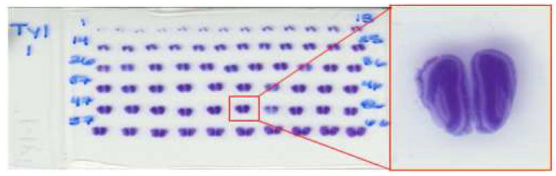
An example of a scanned mouse brain histological glass slide, with one high resolution histological image.
B. 3D Histological volume reconstruction
To reconstruct 3D volume from the histological cross-sections, four steps are applied to the digitized images: image segmentation, center alignment, rigid body alignment, and color normalization. The following sections explain those steps in detail.
1. Image segmentation
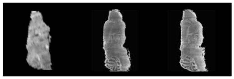
The first step in the process is to extract sub-images, which contain a single cross section from the digitized slides. The connected components on the slides are detected and labeled first, with one individual component containing a single cross-section. Next, sub-images are extracted and ordered, using their position on the slide. Finally, the brain is extracted from each of the sub-images. To achieve this, we have used a level-set method with a dynamic speed function we have proposed for the segmentations of images with weak edges [21]. Initial contours are placed outside the brain area and evolve toward the brain edges. The left panel of Fig. 2 illustrates a typical histological image with the initial contours (the blue circles). The middle panel shows the mask extracted with our segmentation algorithm. The right panel shows the brain extracted from the image.
Fig. 2.
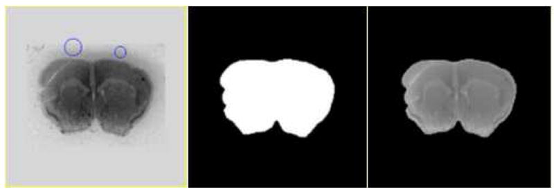
A histological image with the initial contours (left), the mask extracted with the level-set method (middle), and the extracted image (right). This segmentation procedure is the first step used in the reconstruction of 3D histological volumes.
2. Center alignment
In this step, the segmented histological slices are registered to each other sequentially, starting from the first image to the last one, by realigning the center of the slices. This step generates a coarse result and provides a good initialization for the next step. The left panel of Fig. 3 shows the result after this step.
Fig. 3.
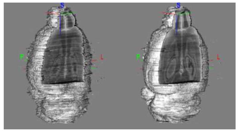
The reconstructed histological volume before registration (left) and after rigid body registration (right). The internal structures are reconstructed accurately after rigid body registration.
3. Rigid body alignment
Next, the slices are registered sequentially using a Mutual Information-based rigid body registration algorithm. A rigid body transformation only includes three parameters: one rotation angle R and a translation vector t = [tx, ty]. The algorithm calculates the optimal parameters R and t through maximizing the Normalized Mutual Information (NMI) using Powell's algorithm [22]:
| (1) |
where A and B' are the target image and the transformed image, respectively, and H (·) is the Shannon entropy of the image, which measures the amount of information in this image viaEq. (2),
| (2) |
where pi (i) is the probability of an intensity value i in the image I.
Although most of the slices can be registered successfully using this method, failures happen because the algorithm converges to an erroneous local minimum. For our data sets, we have observed a 10% error rate. We have also observed that the most critical parameter in our registration algorithm is the number of bins used to compute the joint histograms from which MI is evaluated and we have determined that histograms with 32 bins were the most robust and reliable. Based on this observation we used 32 bins as the default value to compute the histograms but we have developed an algorithm that modifies the number of bins if it is determined that the registration is stuck in an erroneous local minimum. To detect whether or not the algorithm has reached an erroneous local minimum, a threshold on the MI is used. Through experimentation, we have determined that if the MI between two successive slices is above this threshold, the registration has converged to a visually acceptable result. If it is below, the algorithm has generally converged toward the wrong solution. After each slice-to-slice registration the final MI is checked. If it is below the threshold, which is the same for all slices and all volumes, the algorithm is restarted with 8, 16, 64, and 128 bins. The registration that leads to the largest MI is selected as the correct one.
This approach reduced the error rate to 1.5%. The remaining mis-registered cases were identified visually and realigned manually. The right panel of Fig. 3 shows the reconstructed volume after this step.
4. Color normalization
As discussed earlier, not only spatial normalization, but also color normalization is necessary to reconstruct the histological volumes. This is so because individual slices can absorb more or less cresyl violet stain during the histological slice preparation. This, in turn, affects the overall intensity of a slice as well as the contrast between structures.
In this work, we use a weighted histogram specification method on each of the R (red), G (green) and B (blue) channels of the histological images. The standard histogram specification algorithm consists in computing an intensity transformation T that minimizes the difference between the cumulative histogram of a source image to be corrected and a target histogram:
| (3) |
where C is the cumulative histogram function, and Is and It are the reference and target images, respectively.
But, a global optimal intensity histogram (the target histogram) is difficult to find. This is so because different structures are visible in different slices. These slices thus have different intensity distributions and one single target histogram is insufficient to capture the characteristics of all the slices. One solution is to choose a number of target slices spread over the volume and to normalize the intensities block by block. As will be seen, this leads to results that are satisfactory locally but it also produces banding artifacts (i.e., variations in image appearance from one block to the other). Here we propose a method that solves this problem. We start by selecting a number of target slices across the volume. Typically, we choose one target slice every 30 slices (this number was chosen experimentally for our data set) and we normalize slices between these target slices using the intensity histograms of both target slices as follows. Let St be the target slice. For every slice Si ∈ { St ,St+1 } , we compute the intensity transformations between Si and St , and between Si and St+1 :
| (4) |
The final transformation T for Si is then computed as:
| (5) |
where , and , with D the distance between two slices, and v the distance between the two target slices, which has been set to 30. This technique is simple, non-iterative, fully automatic, and we found it to be robust.
Fig. 4 illustrates results obtained with the various intensity normalization schemes we have discussed. Panel (a) shows the stacked slices prior to segmentation and registration in the horizontal orientation. Hence, every column in this panel represents one axial histological slice. Panel (b) shows the histological volume after registration but before intensity normalization. Panel (c) shows the intensity normalization results obtained when only one reference histogram is used. Here, the middle slice has been selected as target and all the other intensity values have been normalized sequentially moving to the left and to the right of the central slice. Clearly, this leads to suboptimal contrast for some of the slices (see for example the reduction in contrast in the cerebellum's region). Panel (d) shows the results when several target histograms are selected and the images normalized block by block. This leads to good results within a block but also to noticeable differences across blocks. Panel (e) shows results obtained with our method. These results show that we have been able to remove intensity and contrast differences between nearby slices while preserving good contrast across the entire volume. To show the robustness of our approach, Fig. 5 illustrates the four histological volumes we have used in this study before (left column) and after (right column) color normalization with our algorithm.
Fig. 4.
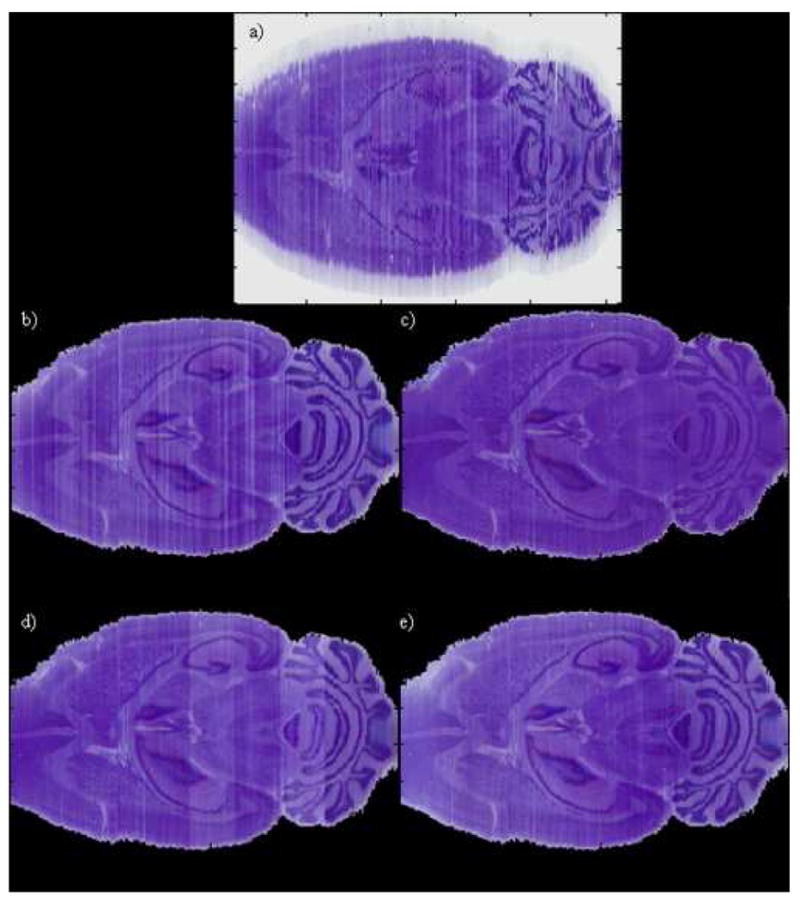
One slice in the 3D reconstructed histological volume after stacking the original histological images (a), after segmentation and registration (b), after color normalization using one single target histogram for the whole volume (c), one target histogram per interval (d), and the method we propose (e).
Fig. 5.
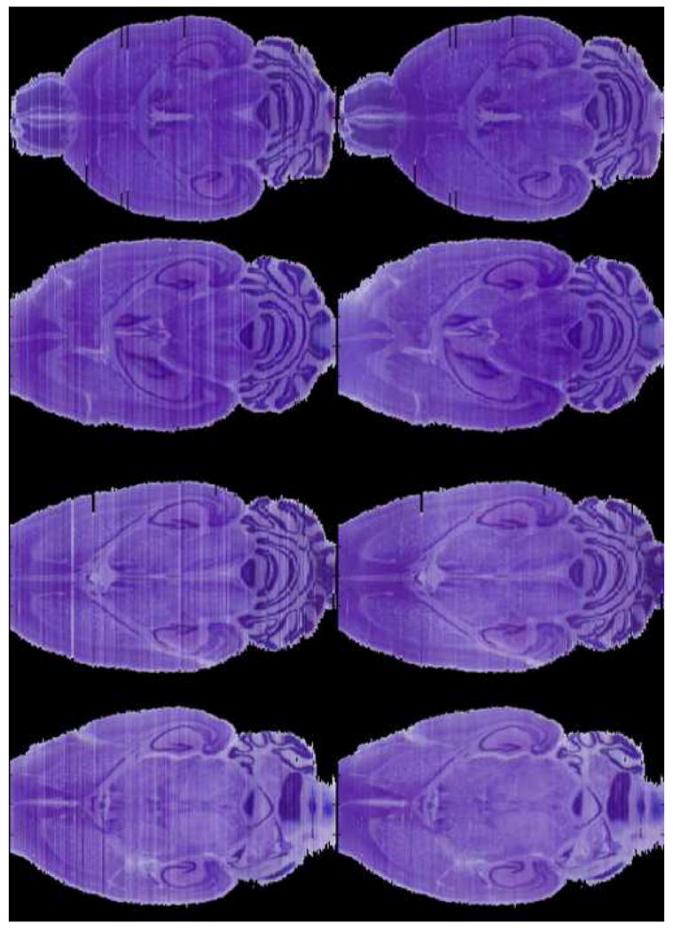
Four reconstructed histological volumes before (left column) and after (right column) color normalization. Inter-slice intensity variations are eliminated in all these four volumes after the color normalization.
Theoretically, the continuous or discrete transformation computed through histogram specification is single-valued and monotonic in an interval. However, in practice, after the discrete transformation, the transformed intensities in one image need to be quantized into integers in the range of [0, 255] to generate a new image. Because of this, multiple intensities in the source image can be mapped into a single intensity in the target image. Moreover, intensity remapping through histogram specification may move pixels from one bin to the other in the intensity histogram used to compute the mutual information between slices. We investigated whether or not intensity normalization has any impact on the registration results. To do so, color normalization was applied to the images before and after rigid body alignment. While the registration algorithm did not fail on the same slices when either of the strategy was used, the rate of failure remained the same at approximately 1.5%. Color normalization was performed before registration to generate all the results presented in this article.
C. Registration of histological volumes to their corresponding MR volume
The next step in the process involves registering histological volumes to their corresponding MR volumes. First, brains are extracted from the MR images using the same level-set algorithm used to separate background and brain regions in the histological images. Next, the two brain volumes are registered. This requires several steps because of the difficulty mentioned in the Introduction section. Namely, when we reconstruct the histological volumes, we stack images consecutively, while maximizing the MI between these slices. This leads to histological volumes whose overall shape does not match exactly the shape of the MR volume as shown in the middle panel of Fig. 6. To address this issue, we first register the MR volume to its histological volume using a rigid-body registration technique. When this is done, we translate each slice in the histological image such that its center of mass coincides with the center of mass of the corresponding MR slice. This is similar to what has been done by Yushkevich et al. [23] and Malandain et al. [16]. We note that these authors added one component to the process to insure a smooth transition between successive transformations. They also used transformations with more degrees of freedom. We did not find this necessary with our data set. This is probably due to the fact that we are dealing with mouse MR images that have a much lower spatial resolution than the monkey and human brain MR images they are using in their studies. The result of this operation is shown on the right panel of Fig. 6. Finally, when the individual slices have been registered to the MR slices, the new histological volume is registered in 3D to the MR volume using a non-rigid registration algorithm [24], which is described in Section II.D.
Fig. 6.
One sagittal slice in one MR volume (left), histological volume after rigid body registration (middle), and histological volume after rigid body registration and realignment of each slice to the corresponding one in the MR volume (right).
Unfortunately, the individual histological volumes obtained with the aforementioned techniques suffer from a series of defects such as tearing or missing segments. One approach is to try to develop more sophisticated reconstruction techniques that can deal with these issues but these are challenging problems. Automatic, robust, and practical solutions will thus be difficult to develop. A practical alternative is to try to combine several individual volumes and generate one synthetic volume that suffers from fewer defects, which is the approach we have investigated.
D. Creation of the average histological volume
The method we have used is a technique that has been proposed for the creation of population averages [26]. In this context, one computes one image volume (e.g., a human brain volume), which is representative of a population as a whole. These averages can then be used to compare populations. Even though our immediate objective is not to compare populations, averaging image volumes can help alleviate defects in individual histological volumes, as these defects are random and occur at different locations in each volume.
The averaging method we have used is illustrated in Fig. 7. First, one histological volume is selected as a reference (it has been shown [26] that the selection of the reference does not affect the average result) and all the other volumes are registered to this reference image, using a rigid registration algorithm first. A non-rigid registration algorithm is then applied to each volume and two deformations fields, which are inverses of each other, are produced. The first, which we call the forward field, permits the registration of a volume to the reference volume. The second, which we call the reverse field, permits the registration of the reference volume to one of the other volumes. Once the deformation fields have been computed, an intensity average is computed. This is done by applying the forward fields to each of the volumes and averaging the resulting volumes. Next, an average shape volume is computed. This is done by first averaging the reverse deformation field. The average reverse deformation field is then applied to the intensity average to produce a new reference. Note that this new reference volume is a “virtual volume”; i.e., it is different from all the original histological volumes. All the volumes are again registered to this new reference volume and the process is repeated until convergence. The experiments we conducted show that after 3 or 4 iterations, both the intensity and the deformation field of the average model remain constant, and the process converges.
Fig. 7.
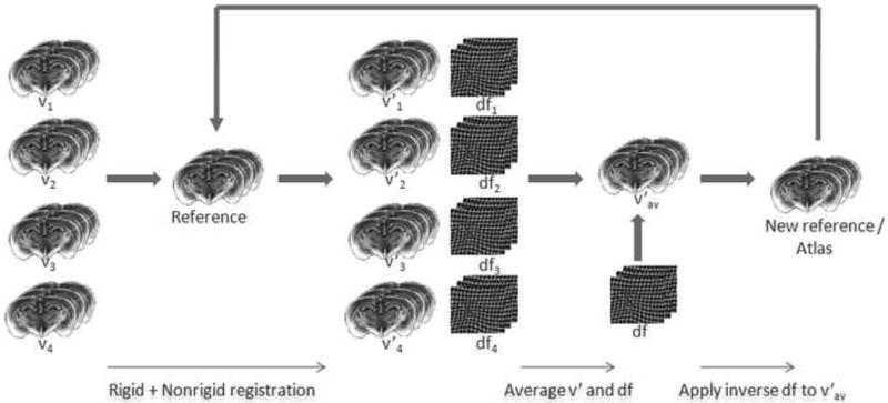
Flow chart of the algorithm used to generate the average volume. The individual reconstructed volumes are averaged using this algorithm and a virtual volume with high SNR is generated (adapted from [26]).
As is the case for inter-slice intensity normalization, we use a histogram specification method to normalize intensities across volumes. Here, a single target histogram is computed from the target volume; the intensities in the other reconstructed volumes are normalized to match the target one.
The algorithm we have used to compute the non-rigid registration is an MI-based algorithm we have proposed, which we call ABA for adaptive bases algorithm [24]. This algorithm models the deformation field that registers the two images as a linear combination of radial basis functions (RBFs) with finite support:
| (6) |
where x is a coordinate vector in ℜd, with ℜd the d-dimensional real space, and d the dimensionality of the images. Φ is one of Wu's compactly supported positive radial basis functions [25], and the ci 's are the coefficients of these basis functions. The coefficients of the radial basis functions are computed through maximizing the Normalized Mutual Information. This algorithm implements several improvements over other existing mutual information-based non-rigid registration algorithms. These include working on an irregular grid, adapting the stiffness of the transformation locally, decoupling a very large optimization problem into several smaller ones, and deriving schemes to guarantee the topological correctness of the transformations.
The algorithm is applied using a multiscale and multi resolution approach. The resolution is related to the spatial resolution of the images. The scale is related to the region of support and the number of basis functions. Typically, the algorithm is started on a low-resolution image with few basis functions with large support. The image resolution is then increased and the support of the basis function decreased. Following this approach, the transformations become more and more local as the algorithm progresses. The algorithm progresses until the highest image resolution and highest scale are reached.
In this algorithm, the transformation is kept topologically correct through imposing a constraint on the difference between the coefficients of adjacent basis functions. The concept is simple: if the coefficients of adjacent basis functions vary widely, the resulting deformation field changes rapidly. Hence, it is possible to spatially adapt the stiffness characteristics of the transformation through creating a stiffness map. The stiffness map has the same dimensions as the original images and associates different stiffness thresholds with different regions. In previous work [27], we have shown this to be of value for registering brain volumes with large space-occupying lesions or with extremely large ventricles. We found it to be useful for this application as well. Looking at Fig. 8, one observes that the images are made of two distinct regions. The first one is the cerebellum in which layers of white and gray matter are clearly visible; these create distinct features that can guide a non-rigid, intensity-based, registration algorithm. The second region encompasses the rest of the brain. In this region, contrast is weaker and internal structures and substructures do not show clearly defined edges. It is well known that intensity-based algorithms as the one we use need to be regularized more over uniform regions than they need to be on regions with a lot of edge information. Hence, we have used a simple binary stiffness map in this study. Stiffness is smaller over the cerebellum region than it is over the rest of the brain region. In other words, the deformation field is regularized more over regions in which edge information is not very reliable (the brain) and less over regions in which edge information is more reliable (the cerebellum).
Fig. 8.
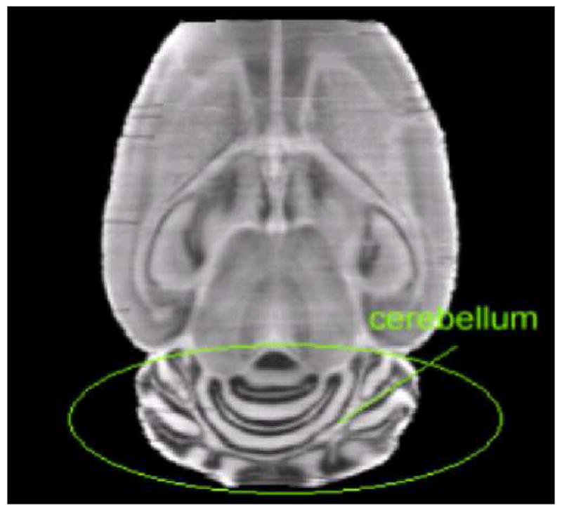
One slice in a histological volume. This image shows that the cerebellum area contains more edge information than the rest of the image.
The effect of using two stiffness values is shown in Fig. 9. The left panel in this figure shows one slice in the reference volume. To create the middle panel, another volume was first registered to the reference volume using one single stiffness value, which produces good results over the brain region. The reference volume and the registered volume were then averaged. The middle panel shows one slice in this average volume. The right panel shows the same but when two stiffness values are used (the transformation is more elastic over the region of cerebellum). This figure shows that the two volumes are aligned more accurately over the region of cerebellum when two stiffness values are used, thus suggesting a better registration.
Fig. 9.
One slice in the reference volume (left), in the average of two volumes registered with one single stiffness value (middle), and in the average of two volumes registered with two stiffness values (right).
E. Creation of the average MR volume
A single MR volume can be created from the four MR volumes acquired in this study in two ways. The first one involves repeating the procedure described above for the creation of the average histological volume. If this approach is used, one of the MR volumes is selected as the original target. The remaining volumes are registered to this first target, the deformation field averaged, a new MR target is created, and the process is repeated until convergence. The second approach relies on the histological volumes to create the MR atlas. First, each MR volume is registered to its own histological atlas. Then, the average histological atlas is created as described earlier. Finally, the transformation that registers each individual histological volume to the average histological atlas is applied to its own registered MR volume to achieve the average MR volume. Results obtained with the two methods will be compared in the next section.
F. Algorithms Implementation
The main registration algorithms (rigid and non-rigid) were implemented in the C programming language. The segmentation algorithm, which was used to extract the mouse brains from the background, was also implemented in the C language. Other algorithms, such as the one used for center alignment and color normalization, were implemented in MATLAB (Mathworks Inc., Sherborn, MA). To implement the strategy that improves the accuracy of rigid registration described in Section II.B.3, MATLAB was also employed to call the rigid registration algorithm, check the values of MI, and modify the number of bins.
III. Results
A. Average histological and MR volumes
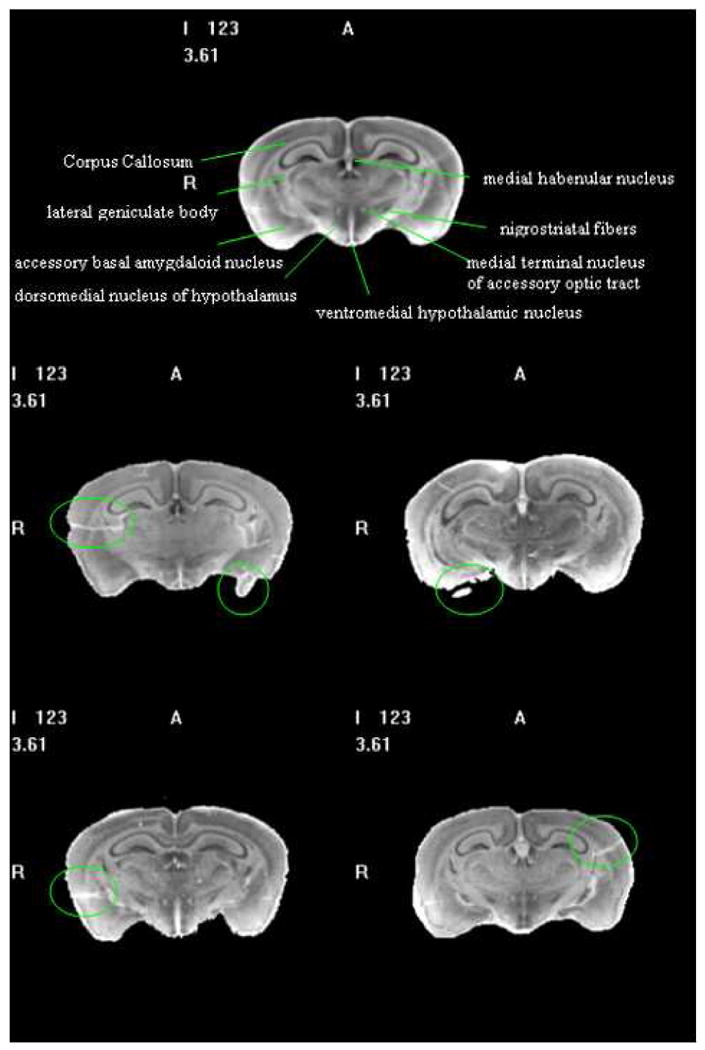
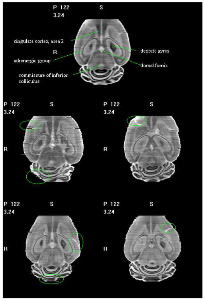
Fig. 10 and Fig. 11 illustrate the results we have obtained with our averaging method. In these figures, the top panel shows one slice in the average. The other panels show the same slice in the four individual volumes used in this study. These figures show two important things. First, defects that are apparent in the individual volumes have virtually disappeared from the average volume. Second, small structures, such as the medial terminal nucleus of the accessory optic tract, the nigrostriatal fibers, or the lateral geniculate body, are clearly visible in the average volume despite being barely visible in the individual image volumes.
Fig. 10.
One axial slice from the averaged histological volume (1st row) with labeled structures, and individual volumes (2nd – 3rd rows). Green circles mark some defects in the individual volumes. Defects are eliminated and small structures are more visible in the averaged volume.
Fig. 11.
One coronal slice in the averaged histological volume (1st row) with labeled structures, and individual volumes (2nd – 3rd rows). Green circles mark some defects in the individual volumes.
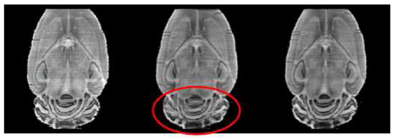
Fig. 12 shows the improvement one can expect when using several histological volumes. The left panel shows an average obtained with two histological volumes, the middle panel is the average obtained with three histological volumes, and the right panel is the average obtained with all four volumes. Green marks show some defects that appeared in the first two averages, but disappeared in the third average. The red mark shows one artifact existing in the third average. Although new defects may be brought into the average, clearly, increasing the number of volumes used to compute the average generally reduces the defects visible in the average and increases its overall signal-to-noise ratio (SNR).
Fig. 12.
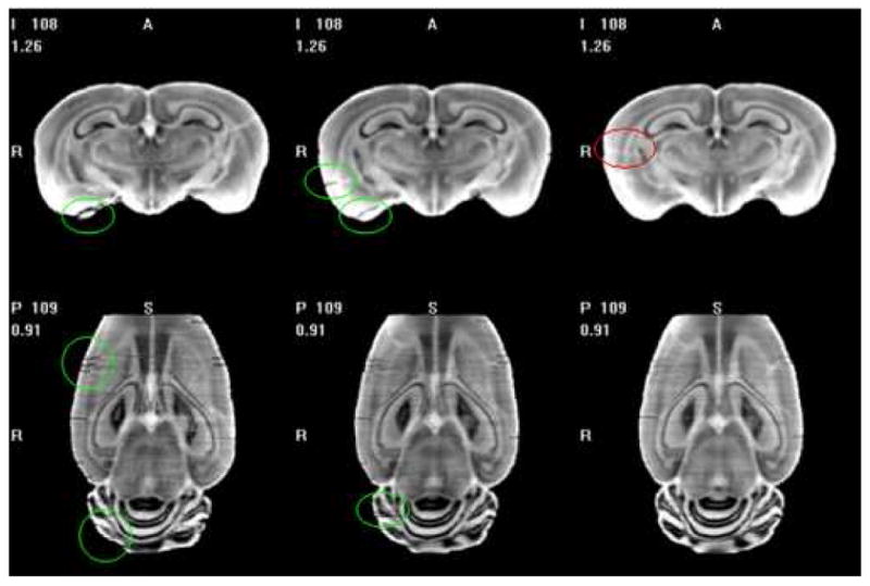
Slices in the average volumes generated using two (left), three (middle) and four (right) individual volumes. Comparing the atlases obtained by different numbers of volumes, we find the SNR of the averaged volume is improved with more individual volumes.
Fig. 13 compares average MR volumes obtained with the two approaches described in Section II.E. The left panel in the image shows one slice in one of the original volumes. The middle panel shows one slice in the average MR volume obtained when the histological images are used and the right panel shows a slice in the average MR volume obtained when MR images alone are used. The right panel is blurrier than the middle one, suggesting that using the histological image volumes improves the registration process. This finding is not very surprising. Indeed, contrast and visibility of internal brain structures are substantially lower in MR images than they are in the histological images. Accurate inter-subject non-rigid registration is thus more difficult for MR images than it is for histological images. When the histological images are used for atlas creation, the only non-rigid registration applied to the MR images is the last step in the intra-subject MR-histological registration process. Typically, this only requires small displacements that improve the results obtained with the rigid-body step. This is a much simpler non-rigid registration problem than the inter-subject registration step required to register MR volumes to each other directly.
Fig. 13.
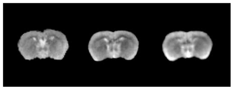
One slice in the original MR volume (left), in the average MR volume obtained using the histological volumes (middle), and the average MR volume obtained by registering MR volumes directly (right).
B. Validation
The MR-histology atlas pair we have created can be used to facilitate the visual interpretation of the MR image as well as to perform automatic volumetric measurements on these images. To validate our approach and demonstrate the usefulness of this atlas we first use a leave-one-out approach to qualitatively show that the registration of the atlas with an MR volume produces accurate results. We then use the same approach to quantitatively assess the accuracy of volumetric measurements for structures that are not easily discernible in the MR images. We complement this validation study with another one performed on an additional ten MR volumes in which we segment structures that are discernible in the MR images.
1. Qualitative evaluation
To evaluate our method qualitatively we used the following approach. First, one MR-histological atlas pair was created with three of the volumes for which we have both MR and histological data. The MR volume in this pair was registered to the fourth MR volume for which we have both MR and histological data. The transformation, which registers the MR atlas to the fourth MR volume, was then applied to the histological atlas, and the deformed atlas was compared to the fourth histological volume. This method permits to judge the quality of the registration between the MR atlas and a new MR volume on structures that are not visible on the MR images. Fig. 14 shows results on a few slices. In this figure, the left panels are slices in the fourth MR volume. The middle panels are the histological slices in the histological volume associated with the fourth MR volume. The right panels are the corresponding slices in the histological atlas registered to the fourth MR volumes using the MR atlas. Contours have been drawn manually on the right panels and copied on the corresponding middle panels. These contours show a very good agreement between the histological volumes, thus demonstrating that accurate registration between MR volumes is achievable. It also shows that information such as the position of anatomic structure not visible in the MR can be inferred automatically from a histological atlas.
Fig. 14.
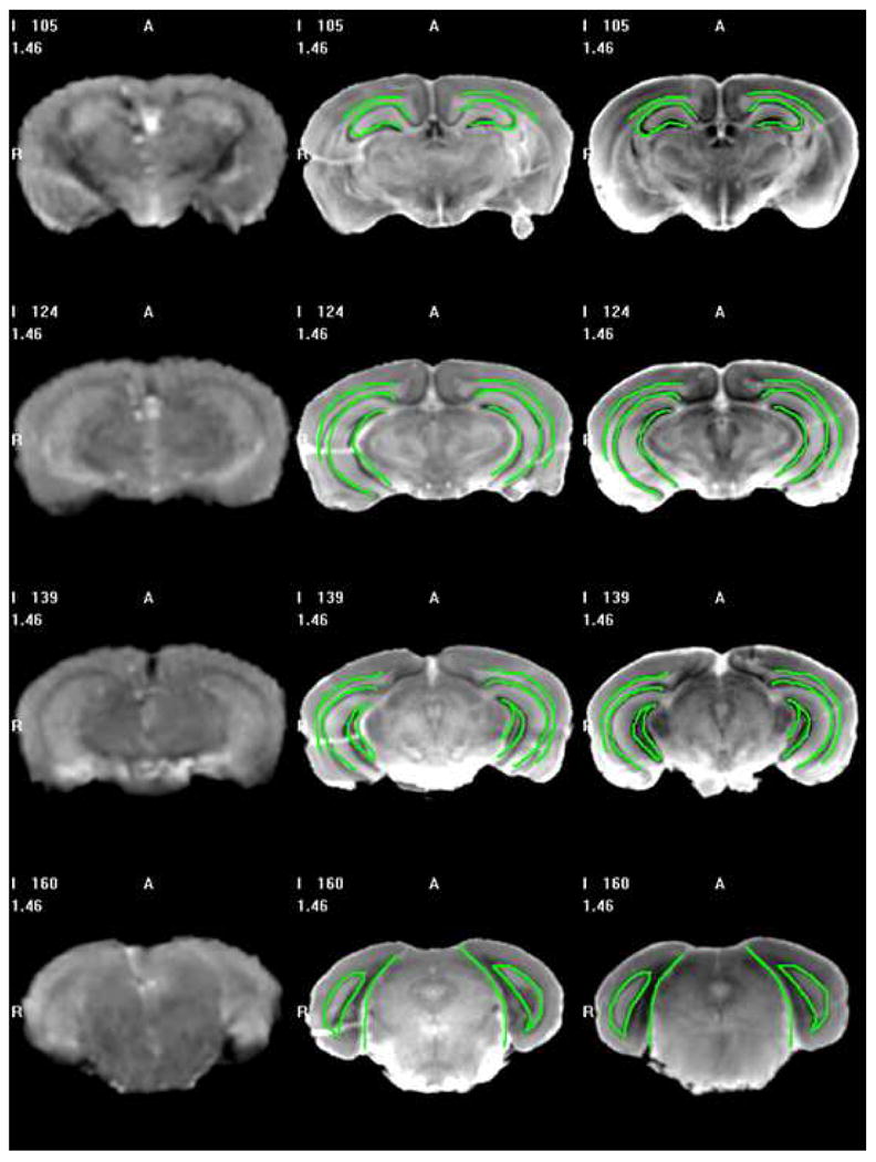
Slices in the 4th MR volume (left column), the 4th histological volume (middle column), and the histological atlas (right column) obtained using a leave-one-out method. The contours were drawn manually on the images shown on the right and copied on the images shown in the middle.
2. Quantitative validation on structures not visible in the MR images
To evaluate the usefulness of our MR-histology atlas for the quantitative analysis of MR images we first used the same leave-one-out strategy described in the previous section, i.e., we have created four pairs of MR-histology atlases. Each of these was created using only three of the four MR-histological volume pairs and tested on the fourth one. To test our approach for volumetric measurements, the hippocampus was first delineated manually in each of the histological atlases. Next, the MR atlases (created with three volumes) were registered to the fourth MR volume, which was already registered to its own histological volume. The deformation field computed using this method was then used to project the hippocampus contours from the histological atlas onto the fourth histological volume. Manual and automatic contours for the fourth histological volumes were then compared. This approach permits evaluating the accuracy of our atlas-based segmentation method in four volumes. Fig. 15 shows hippocampus contours we have obtained automatically and contours obtained manually superimposed on the MR volume not used to create the atlas (left panels) and on the corresponding histological volume (right panels). To validate the results quantitatively, manual and automatic contours were compared using the Dice similarity index [28] defined as follows:
Fig. 15.
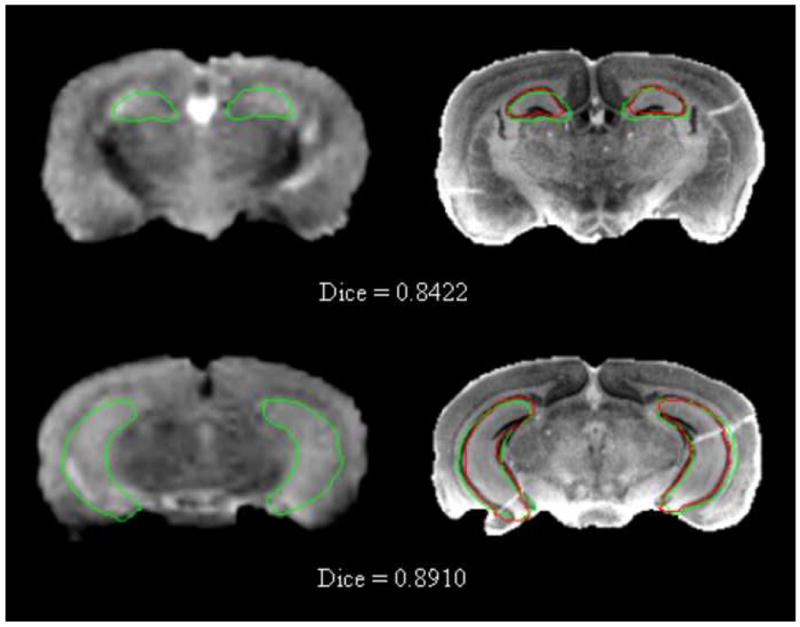
Hippocampus contours obtained automatically (green) and manually (red) are superimposed on the MR volume (left column) and on the corresponding histological volume (right column).
| (7) |
where n{.} indicates the number of voxels within a region and A and M are the automatic and manual contours. Fig. 16 shows this Dice similarity result. Dice values above 0.7 are customarily considered indicative of a good agreement between contours [29].
Fig. 16.
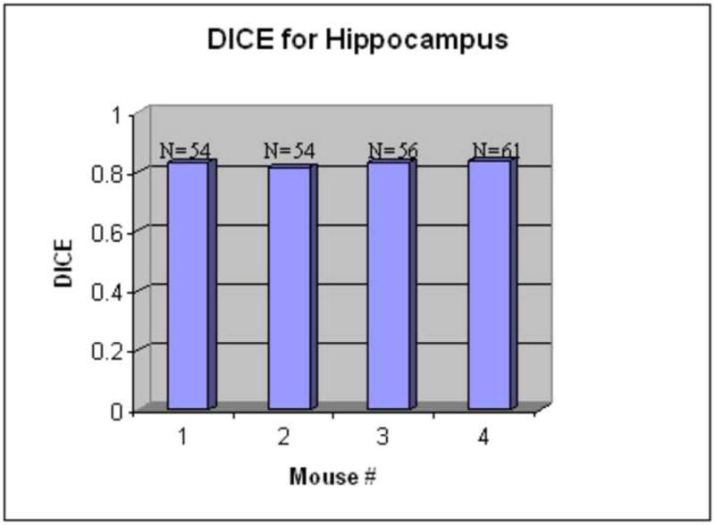
The Dice similarity index for hippocampus structures (N: the number of slices). The Dice values are around 0.8, which indicates the accuracy of the atlas-based segmentation.
3. Quantitative validation on structures visible in the MR images
In the previous section we have validated our approach on structures that are not visible in the MR images. This is possible because we have an associated histological volume for each of the MR volumes. But this validation was limited to the four data sets for which we had both MR and histological information. To further evaluate the atlases we tested the accuracy of automatic volumetric measurements on additional MR volumes acquired with the same imaging protocol described in Section II.A. Because we did not have associated histological volumes, we limited our analysis to structures, which could be visually identified and manually delineated in the MR images. Three structures were manually contoured in each of the ten volumes: the left lobe, the right lobe, and the cerebellum. These structures were also delineated in the atlas (here we use an MR-histology atlas created with the four data sets). The atlas was registered to all the other volumes and 3D structures delineated in the atlas were deformed with the computed deformation field. Contours obtained automatically were compared to the manual contours using the Dice similarity index. Table 1 shows the Dice values for all ten mice. The mean values for all three structures are above 0.9, which indicates an excellent agreement between the automatic contours and the manually segmented contours. Those mean values are larger than the Dice values obtained for the hippocampus contours in the previous validation experiment. The reason is that, compared with the regions of hippocampus, these three structures have clearer edges in the MR images, which improves the accuracy of intensity-based methods such as the one used in this work.
Table 1.
Dice coefficients for three structures in the mouse brains.
| Left lobe | Right lobe | Cerebellum | # of slices (left/right) |
# of slices (cerebellum) |
|
|---|---|---|---|---|---|
| # 01 | 0.9589 | 0.9578 | 0.9377 | 15 | 3 |
| # 02 | 0.9695 | 0.9643 | 0.9351 | 16 | 3 |
| # 03 | 0.9729 | 0.9707 | 0.9310 | 17 | 3 |
| # 04 | 0.9687 | 0.9621 | 0.9135 | 16 | 3 |
| # 05 | 0.9600 | 0.9587 | 0.9004 | 15 | 3 |
| # 06 | 0.9653 | 0.9560 | 0.9144 | 14 | 3 |
| # 07 | 0.9603 | 0.9597 | 0.9291 | 16 | 3 |
| # 08 | 0.9705 | 0.9663 | 0.9192 | 14 | 3 |
| # 09 | 0.9724 | 0.9658 | 0.9109 | 15 | 4 |
| # 10 | 0.9722 | 0.9700 | 0.8750 | 16 | 3 |
| Mean | 0.9671 | 0.9632 | 0.9166 | 15.4 | 3.1 |
IV. Discussion
Defects in individual histological slices are unavoidable and difficult to correct because they involve tearing, missing parts, or folding. The study we have conducted has shown that a very practical solution to reconstruct 3D histological volumes of high quality is to use more than one reconstructed histological volume and to create one single volume from these through non-rigid registration. The accuracy of our non-rigid registration is such that the average it produces has a higher signal-to-noise ratio than any of the individual volumes used for its creation. This permits the clear visualization of structures that are not easily discernable in the individual volumes. Also, defects in individual volumes become less apparent in the average one because of the intensity averaging we perform. Some defects remain in the atlas we have created with our four MR-histology data sets, which makes it less than a gold standard, but these are such that it is unlikely that they substantially affect the volumetric measurement we have made. Adding more MR-histology data sets would further improve the quality of the atlas. As noted in the introduction, intensity normalization is an important component for the reconstruction of histological volumes. Others have proposed methods that are somewhat complex, often requiring iterative optimization steps and parameter adjustments. The new method we propose is based on a standard histogram specification technique. With the modification we have developed it leads to satisfactory results while being simple, fast, and parameter free (except for the selection of the number of target histograms, which is not critical). The method we use to realign histological slices to each other is largely automatic albeit we have observed a failure rate around 1.5%. One possible way to address the issue would be to restart the rigid body registration algorithm from different starting points to steer it away from erroneous local minima and to select the solution that produces the largest MI. Using our histological atlases, we have shown that atlas-based segmentation methods permit accurate volumetric measurements of mice MR images both on structures that are visible in these images and on structures that are difficult to discern. An immediate, and promising, application of this technique involves the segmentation of brain structures in mouse populations that have been, for example, genetically manipulated—an area of active investigation to understand the adult and developing mammalian central nervous system [30-32]. Others have developed digital MR atlases [6][7][33]. These are built directly from 3D tomographic volumes that are acquired with very long acquisition sequences. While results obtained with these approaches are excellent, there remains a place for histological atlases. Indeed, histology can still provide a spatial resolution that is far superior to what is achievable with MR and various histology stains can be used to visualize nuclei or cell surface receptors that cannot be seen in MR images. It is thus likely that histology will remain the standard for many years to come. But, the creation of good quality histological cross-sections is a difficult task that requires experience and skills. The method proposed herein permits the reconstruction of high quality volumes even if the raw data is less than perfect.
Acknowledgments
The authors gratefully acknowledge support from SAIRP U24 CA126588, NIBIB 2R01 EB000214-15A1, and 1K25 EB005936. We thank Mr. Richard Baheza for expert technical MRI assistance.
Footnotes
Publisher's Disclaimer: This is a PDF file of an unedited manuscript that has been accepted for publication. As a service to our customers we are providing this early version of the manuscript. The manuscript will undergo copyediting, typesetting, and review of the resulting proof before it is published in its final citable form. Please note that during the production process errors may be discovered which could affect the content, and all legal disclaimers that apply to the journal pertain.
References
- 1.Gillies RJ, Bhujwalla ZM, Evelhoch JL, Garwood M, Neeman M, Robinson SP, Sotak CH, Van Der Sanden B. Applications of maagentic resonance in model systems: Tumor biology and physiology. Neoplasia. 2000;2:139–51. doi: 10.1038/sj.neo.7900076. [DOI] [PMC free article] [PubMed] [Google Scholar]
- 2.Evelohoch JL, GIllies RJ, Karczmar GS, Koutcher JA, Maxwell RJ, Nalcioglu O, Raghunand N, Ronen SM, Ross BD, Swartz HM. Applications of magnetic resonance in model systems: Cancer therapeutics. Neoplasia. 2000;2:152–65. doi: 10.1038/sj.neo.7900078. [DOI] [PMC free article] [PubMed] [Google Scholar]
- 3.Yan GP, Robinson L, Hogg P. Magnetic resonance imaging contrast agents: Overview and perspectives. Radiography. 2007;12:e5–e19. [Google Scholar]
- 4.Daldrup-Link HE, Meier R, Rudelius M, Piontek G, Piert M, Metz S, Settles M, Uherek C, Wels W, Schlegel J, Rummeny EJ. In vivo tracking of genetically engineered, anti-HER2/neu directed natural killer cells to HER2/neu positive mammary tumors with magnetic resonance imaging. Eur Radiology. 2005;15:4–13. doi: 10.1007/s00330-004-2526-7. [DOI] [PubMed] [Google Scholar]
- 5.Hakumäki JM, Brindle KM. Techniques: Visualizing apoptosis using nuclear magnetic resonance. Trends in Pharmacol Science. 2003;24:146–9. doi: 10.1016/S0165-6147(03)00032-4. [DOI] [PubMed] [Google Scholar]
- 6.Chan E, Kovacevíc N, Ho SK, Henkelman RM, Henderson JT. Development of a high resolution three-dimensional surgical atlas of the murine head for strains 129S1/SvImJ and C57Bl/6J using magnetic resonance imaging and micro-computed tomography. Neuroscience. 2007;144(2):604–15. doi: 10.1016/j.neuroscience.2006.08.080. [DOI] [PubMed] [Google Scholar]
- 7.MacKenzie-Graham A, Lee EF, Dinov ID, Bota M, Shattuck DW, Ruffins S, Yuan H, Konstantinidis F, Pitiot A, Ding Y, Hu G, Jacobs RE, Toga AW. A multimodal, multidimensional atlas of the C57BL/6J mouse brain. J Anat. 2004;204(2):93–102. doi: 10.1111/j.1469-7580.2004.00264.x. [DOI] [PMC free article] [PubMed] [Google Scholar]
- 8.Deverell MH, Salisbury JR, Cookson MJ, Holman JG, Dykes E, Whimster F. Three-dimensional reconstruction: methods of improving image registration and interpretation. Anal Cell Pathol. 1993;5:253–263. [PubMed] [Google Scholar]
- 9.Rydmark M, Jansson T, Berthold CH, Gustavsson T. Computer assisted realignment of light microgragh images from consecutive sections series of cat cerebral cortex. J Microsc. 1992;165:29–47. doi: 10.1111/j.1365-2818.1992.tb04303.x. [DOI] [PubMed] [Google Scholar]
- 10.Cohen FS, Yang Z, Huang Z, Nissanov J. Automatic matching of homologous histological sections. IEEE Trans Biomed Engng. 1998;45(5):642–649. doi: 10.1109/10.668755. [DOI] [PubMed] [Google Scholar]
- 11.Kay PA, Robb RA, Bostwick DG, Camp JJ. Robust 3-D reconstruction and analysis of microstructures from serial histologic sections, with emphasis on microvessels in prostate cancer. Visual Biomed Comput, Lecture Notes in Computer Science. 1996;1131:129–134. [Google Scholar]
- 12.Rangarajan A, Chui H, Mjolsness E, Pappu S, Davachi L, Goldman-Rakic P, Duncan J. A robust point-matching algorithm for autoradiograph alignment. Med Image Anal. 1997;1(4):379–398. doi: 10.1016/s1361-8415(97)85008-6. [DOI] [PubMed] [Google Scholar]
- 13.Ourselin S, Roche A, Subsol G, Pennec X. Automatic Alignment of Histological Sections. International Workshop on Biomedical Image Registration, WBIR; 1999. pp. 1–13. [Google Scholar]
- 14.Ourselin A, Roche A, Subsol G, Pennec X, Ayache N. Reconstructing a 3-D structure from serial histological sections. Image Vision Comput. 2001;19(12):25–31. [Google Scholar]
- 15.Ourselin S, Bardinet E, Dormont D, Malandain G, Roche A, Ayache N, Tande D, Parain K, Yelnik J. Fusion of Histological Sections and MR Images: Towards the Construction of an Atlas of the Human Basal Ganglia. The 4th International Conference on Medical Image Computing And Computer-Assisted Intervention; 2001. pp. 743–751. [Google Scholar]
- 16.Malandain G, Bardinet É, Nelissenc K, Vanduffel W. Fusion of autoradiographs with an MR volume using 2-D and 3-D linear transformations. NeuroImage. 2004;23:111–127. doi: 10.1016/j.neuroimage.2004.04.038. [DOI] [PubMed] [Google Scholar]
- 17.Dauguet J, Mangin JF, Delzescaux T, Frouin V. Robust inter-slice intensity normalization using histogram scale-space analysis. Medical Image Computing and Computer Assisted Intervention. 2004;3216:242–249. [Google Scholar]
- 18.Chakravarty MM, Bertrand G, Hodge CP, Sadikot AF, Collins DL. The creation of a brain atlas for image guided neurosurgery using serial histological data. Neuroimage. 2006;30:359–76. doi: 10.1016/j.neuroimage.2005.09.041. [DOI] [PubMed] [Google Scholar]
- 19.Gonzales R, Wintz P. Digital Image Processing. Addison-Wesley; 1977. [Google Scholar]
- 20. http://www.mbl.org/tutorials/MBLTrainingManual/index.html.
- 21.Dawant BM, Pan S, Li R. Robust Segmentation of Medical Images Using Geometric Deformable Models and a Dynamic Speed Function. Lecture Notes in Computer Science (LNCS 2208) Medical Image Computing and Computer-assisted Intervention. 2001:1040–1047. [Google Scholar]
- 22.Press W, Teukolsky S, Vetterling W, Flannery B. Numerical Recipes in C The Art of Scientific Computing. 2nd. Cambridge, U.K.: Cambridge Univ. Press; 1994. [Google Scholar]
- 23.Yushkevich PA, Avants B, Ng L, Hawrylycz M, Burstein PD, Zhang H, Gee JC. 3D Mouse Brain Reconstruction from Histology Using a Coarse-to-Fine Approach. Proc Third International Workshop of WBIR; 2006. pp. 230–237. [Google Scholar]
- 24.Rohde GK, Aldroubi A, Dawant BM. The adaptive bases algorithm for intensity-based nonrigid image registration. IEEE Trans Med Imaging. 2003;22(11):1470–1479. doi: 10.1109/TMI.2003.819299. [DOI] [PubMed] [Google Scholar]
- 25.Wu Z. Multivariate compactly supported positive definite radial functions. Adv. Comput. Math. 1995;4:283–292. [Google Scholar]
- 26.Guimond A, Meunier J, Thirion JP. Average brain models: A convergence study. Comp Vision Image Understand. 2000;77:192–210. [Google Scholar]
- 27.Duay V, D'Haese P, Li R, Dawant BM. Non-Rigid Registration Algorithm With Spatially Varying Stiffness Properties. ISBI. 2004:408–411. [Google Scholar]
- 28.Bartko JJ. Measurement and reliability: Statistical thinking considerations. Schizophr. Bull. 1991;17:483–489. doi: 10.1093/schbul/17.3.483. [DOI] [PubMed] [Google Scholar]
- 29.Zijdenbos AP, Dawant BM, Margolin RA, Palmer AC. Morphometric analysis of white matter lesions in MR images: Method and validation. IEEE Trans Med Imag. 1994;13(4):716–724. doi: 10.1109/42.363096. [DOI] [PubMed] [Google Scholar]
- 30.Brumwell CL, Curran T. Developmental mouse brain gene expression maps. J Physiol. 2006;575(Pt 2):343–6. doi: 10.1113/jphysiol.2006.112607. [DOI] [PMC free article] [PubMed] [Google Scholar]
- 31.Koester SE, Insel TR. Mouse maps of gene expression in the brain. Genome Biol. 2007;8(5):212. doi: 10.1186/gb-2007-8-5-212. [DOI] [PMC free article] [PubMed] [Google Scholar]
- 32.Lein ES, Hawrylycz MJ, Ao N, Ayres M, Bensinger A, et al. Genome-wide atlas of gene expression in the adult mouse brain. Nature. 2007;445(7124):168–76. doi: 10.1038/nature05453. [DOI] [PubMed] [Google Scholar]
- 33.Ma Y, Hof PR, Grant SC, Blackband SJ, Bennett S, Slatest L, McGuigan MD, Benveniste H. A three-dimensional digital atlas database of the adult C57BL/6J mouse brain by magnetic resonance microscopy. Neuroscience. 2005;135(4):1203–15. doi: 10.1016/j.neuroscience.2005.07.014. [DOI] [PubMed] [Google Scholar]