mStruct: Inference of Population Structure in Light of Both Genetic Admixing and Allele Mutations

Abstract

Traditional methods for analyzing population structure, such as the Structure program, ignore the influence of the effect of allele mutations between the ancestral and current alleles of genetic markers, which can dramatically influence the accuracy of the structural estimation of current populations. Studying these effects can also reveal additional information about population evolution such as the divergence time and migration history of admixed populations. We propose mStruct, an admixture of population-specific mixtures of inheritance models that addresses the task of structure inference and mutation estimation jointly through a hierarchical Bayesian framework, and a variational algorithm for inference. We validated our method on synthetic data and used it to analyze the Human Genome Diversity Project–Centre d'Etude du Polymorphisme Humain (HGDP–CEPH) cell line panel of microsatellites and HGDP single-nucleotide polymorphism (SNP) data. A comparison of the structural maps of world populations estimated by mStruct and Structure is presented, and we also report potentially interesting mutation patterns in world populations estimated by mStruct.

THE deluge of genomic polymorphism data, such as the genomewide multilocus genotype profiles of variable numbers of tandem repeats (i.e., microsatellites) and single-nucleotide polymorphisms (SNPs), has fueled the long-standing interest in analyzing patterns of genetic variations to reconstruct the ancestral structures of modern human populations. Genetic ancestral information can shed light on the evolutionary history and migrations of modern populations (Bowcock et al. 1994; Rosenberg et al. 2002; Conrad et al. 2006). It also provides guidelines for more accurate association studies (Roeder et al. 1998) and is useful for many other population genetics problems (Queller et al. 1993; Hammer et al. 1998; Templeton 2002).

Various methods have been proposed for stratifying population structures on the basis of multilocus genotype information from a set of individuals. For example, Pritchard et al. (2000) proposed a model-based approach implemented in the program Structure, which uses a statistical methodology known as the allele-frequency admixture model to stratify population structures. This model, and admixture models in general arising in genetic and other contexts (Blei et al. 2003), belongs to a more general class of hierarchical Bayesian models known as the mixed membership models (Erosheva et al. 2004). Such a model postulates that an empirical multiple-instance sample, such as the ensemble of genetic markers of an individual, is made up of either independently and identically distributed (iid) instantiations (Pritchard et al. 2000) or spatially coupled (Falush et al. 2003) instantiations, from multiple population-specific fixed-dimensional multinomial distributions of marker alleles [known as allele-frequency profiles, AP (Falush et al. 2003)]. Under this assumption, the admixture model identifies each ancestral population by a specific AP (that defines a unique vector of allele frequencies of each marker in each ancestral population) and displays the fraction of contributions from each AP in a modern individual genome as an admixing vector (also known as an ancestral proportion vector or structure vector) in a structural map over the population sample in question. Figure 1 shows an example of a structural map of four modern populations inferred from a portion of the HapMap multipopulation data set by Structure. In this population structural map, the admixing vector underlying each individual is represented as a thin vertical line of unit length and multiple colors, with the height of each color reflecting the fraction of the individual's genome originated from a certain ancestral population denoted by that color and formally represented by a unique AP. This method has been applied to the Human Genome Diversity Project–Centre d'Etude du Polymorphisme Humain (HGDP–CEPH) Human Genome Diversity Cell Line Panel in Rosenberg et al. (2002) and many other studies, and has unraveled interesting patterns in the genetic structures of the world population. However, even though Structure was originally built on a genetic admixture model, in reality the structural patterns derived by Structure in various studies often turn out to be distinct clusters among the study populations (e.g., Figure 1), which has led many to think of it as a clustering program rather than a tool for uncovering genetic admixing as it was supposed to do. The design limitation of the Structure model behind this issue motivated us to develop a new approach in this article to analyze admixed genetic samples.

Figure 1.—

Population structural map inferred by Structure on HapMap data consisting of four populations.

A recent extension of Structure, known as Structurama (Pella and Masuda 2006; Huelsenbeck and Andolfatto 2007), relaxes the finite dimensional assumption on ancestral populations in the admixture model by employing a Dirichlet process prior over the ancestral allele-frequency profiles. This allows automatic estimation of the maximum a posteriori probable number of ancestral populations. This extension is a useful improvement since it eliminates the need for manual selection of the number of ancestral populations. Anderson and Thompson (2002) address the problem of classifying species hybrids into categories, using a model-based Bayesian clustering approach implemented in the NewHybrid program. While this problem is not exactly identical to the problem of stratifying the structure of highly admixed populations, it is useful for structural analysis of populations that were recently admixed. The BAPS program (Corander et al. 2003) also uses a Bayesian approach to find the best partition of a set of individuals into subpopulations on the basis of genotypes. Parallel to the aforementioned model-based approaches for genomic structural analysis, direct algebraic eigen-decomposition and dimensionality reduction methods, such as the Eigensoft program (Patterson et al. 2006) based on principal components analysis (PCA), offer an alternative approach to explore and visualize the ancestral composition of modern populations and facilitate formal statistical tests for significance of population differentiation. However, unlike the model-based methods such as Structure, where each inferred ancestral population bears a concrete genetic meaning as a population-specific allele-frequency profile, the eigenvectors computed by Eigensoft represent the mutually orthogonal directions in an abstract low-dimensional ancestral space, in which population samples can be embedded and visualized; these eigenvectors can be understood as mathematical surrogates of independent genetic sources underlying a population sample, but lack a concrete interpretation under a generative genetic inheritance model (from here on, we use the term “inheritance model” to describe the process by which a descendant allele is derived from an ancestral allele). Analyses based on Eigensoft are usually limited to two-dimensional ancestral spaces, offering limited power in stratifying highly admixed populations.

This progress notwithstanding, an important aspect of population admixing that is largely missing in the existing methods is the effect of allele mutations between the ancestral and current alleles of genetic markers, which can dramatically influence the accuracy of the structural estimation of current populations. It can also reveal additional information about population evolution, such as the relative divergence time and migration history of admixed populations.

Consider, for example, the Structure model. Since an AP merely represents the frequency of alleles in an ancestral population rather than the actual allelic content or haplotypes of the alleles themselves, the admixture models developed so far on the basis of APs do not model genetic changes due to mutations from the ancestral alleles. Indeed, a serious pitfall of the model underlying Structure, as pointed out in Excoffier and Hamilton (2003), is that there is no mutation model for modern individual alleles with respect to hypothetical common prototypes in the ancestral populations. That means every unique allele in the modern population is assumed to have a distinct ancestral proportion, rather than allowing the possibility of it just being a descendant of some common ancestral allele that can also give rise to other closely related alleles at the same locus of other individuals in the modern population. Thus, while Structure aims to provide ancestry information for each individual and each locus, there is no explicit representation of the “ancestors” as a physical set of “founding alleles.” Therefore, the inferred population structural map emphasizes revealing the contributions of abstract population-specific ancestral proportion profiles, which does not necessarily reflect individual diversity or the extent of genetic changes with respect to the founders. Due to this limitation, Structure does not enable inference of the founding genetic patterns, the age of the founding alleles, or the population divergence time (Excoffier and Hamilton 2003).

The lack of an appropriate allele mutation model in a structural inference program can also compromise our ability to reliably assess the amount or level of genetic admixing in different populations. The Structure model, like several other related models (Blei et al. 2003), is based on the fundamental assumption of the presence of genetic admixing among multiple founding populations. However, as we shall see later, on real population data such as the HGDP–CEPH panel, it produces results that favor clustering individuals into predominantly one allele-frequency profile or another, thus leading us to conclude that there was little or no admixing between the ancestral human populations. We believe that this occurs due to the absence of a mutation model in Structure. While a partitioning of individuals would be desirable for clustering them into groups, it does not offer enough biological insight into the intermixing of the populations.

In this article, we present mStruct (which stands for Structure under mutations), based on a new model: an admixture of population-specific mixtures of inheritance models (AdMim). Statistically, AdMim is an admixture of mixture models, which represents each ancestral population as a mixture of ancestral alleles each with its own inheritance process and each modern individual as an “ancestry vector” (or structure vector) that reflects membership proportions of the ancestral populations. As we explain shortly, mStruct facilitates estimation of both the structural map of populations and the mutation parameters of either SNP or microsatellite alleles under various contexts. A new variational inference algorithm, which is much faster than the MCMC algorithm used for Structure, was developed for estimating the structure vectors and other genetic parameters of interest. We compare our method with Structure on simulated genotype data and on the microsatellite and SNP genotype data of world populations (Rosenberg et al. 2002; Conrad et al. 2006). Our results using microsatellite data reveal the presence of significant levels of genetic admixing among the founding populations underlying the HGDP–CEPH cell line panel, as well as consequences of expansion of humans out of Africa. Our results suggest that the inability of Structure to model mutations during genetic admixing could have caused it to detect correct clustering but very low levels of genetic admixing in each modern population in the HGDP–CEPH data. We also report interesting visualizations of genetic divergence in world populations revealed by the mutation patterns estimated by mStruct. The mStruct software has been implemented in C++ and is available for download at http://www.sailing.cs.cmu.edu/mstruct.html.

THE STATISTICAL MODEL

The mStruct model differs from the Structure model in two main aspects: the representation of ancestral populations and the generative process for sampling a modern individual from the ancestral populations. In this section we describe in detail the statistical underpinning of these two aspects.

Representation of Populations

To reveal the genetic composition of each modern individual in terms of contributions from hypothetical ancestral populations via statistical inference on multilocus genotype data, one must first choose an appropriate representation of ancestral populations. We begin with a brief description of the commonly used representation adopted by Structure, followed by a new representation we propose that allows mutations to be captured.

Population-specific allele-frequency profiles:

Since all markers that are used for population structure stratification are polymorphic in nature, it is not surprising that the most intuitive representation of an ancestral population is a set of frequency vectors for all alleles observed at all the loci. Specifically, we can represent an ancestral population k by a unique set of population-specific multinomial distributions , where is the vector of multinomial parameters, also known as an AP (Falush et al. 2003), of the allele distribution at locus i in ancestral population k; denotes the total number of observed marker alleles at locus i; and I denotes the total number of marker loci. This representation, known as population-specific allele-frequency profiles, is used by the program Structure.

Population-specific mixtures of ancestral alleles:

An AP does not enable us to model the possibility of mutations; i.e., there is no way of representing a situation where two observed alleles might have been derived from a single ancestral allele by two different mutations. This possibility can be represented by a genetically more realistic statistical model known as the population-specific mixture of ancestral alleles (MAA). For each locus i, an MAA for ancestral population k is a set consisting of three components: (1) a set of ancestral (or founder) alleles , which can differ from their descendant alleles in the modern population; (2) a mutation parameter associated with the locus, which can be further generalized to be allele-specific if necessary; and (3) an AP , which now represents the frequencies of the ancestral alleles. Here L_i denotes the total number of ancestral alleles at loci i, which is different from in the previous section, which denotes the total number of observed alleles at loci i. By explicitly associating a mutation model with an ancestral population, we can now capture mutation events as described above. It is important to note that the mutation parameter δ is not the mutation rate commonly referred to in the literature. As we shall see later, it is a measure of the variability of a locus that can be described approximately as the combined effect of the per-generation mutation rate and the age of the population.

An MAA is strictly more expressive than an AP, because the incorporation of a mutation model helps to capture details about the population structure that an AP cannot; and the MAA reduces to the AP when the mutation rates (and hence the mutation parameters) become zero and the founders are identical to their descendants. MAA is also arguably more realistic because it allows mutation rates (and mutation parameters) to be different for different founder alleles even within the same ancestral population, as is commonly the case with many genetic markers. For example, the mutation rates for microsatellite alleles are believed to be dependent on their length (number of repeats). As we shall show shortly, with an MAA, one can examine the mutation parameters corresponding to each ancestral population via Bayesian inference from genotype data; this might enable us to infer the age of alleles and also estimate population divergence times subject to a calibration constant.

Let i ∈ {1,…, I} index the position of a locus in the study genome, n ∈ {1,…, N} index an individual in the study population, and e ∈ {0, 1} index the two possible parental origins of an allele (in this study we do not require strict phase information of the two alleles, so the index e is used merely to indicate ploidy of the data). Under an MAA specific to an ancestral population k, the correspondence between a marker allele and a founder is not directly observable. For each allele founder , we associate with it an inheritance model p(· | , ) from which descendants can be sampled. Then, given specifications of the ancestral population from which is derived, which is denoted by hidden indicator variable , the conditional distribution of under an MAA follows a mixture of population-specific inheritance models:

(1)

Comparing to the counterpart of this function under AP, , we can see that the latter cannot explicitly model allele diversities in terms of molecular evolution from the founders.

A New Admixture Model for Population Structure

Admixtures are useful for modeling objects (e.g., human beings), each comprising multiple instances of some attributes (e.g., marker alleles), each of which comes from a (possibly different) source distribution P_k(· | Θ^k), according to an individual-specific admixing vector (a.k.a. structure vector) . The structure vector represents the normalized contribution from each of the source distributions {P_k; k = 1:K} to the object in question. For a single data set, all the structure vectors are assumed to be samples from an underlying structure prior with parameter α. For example, for every individual, the alleles at all loci may be inherited from founders in different ancestral populations, each represented by a unique distribution of founding alleles and the way they can be inherited. Formally, this scenario can be captured in the following generative process:

• 1. For each individual n, draw the admixing vector , where P(· | α) is a prechosen structure prior.

• 2. For each marker allele :

• 2.1, draw the latent ancestral-population-origin indicator ;

• 2.2, draw the allele .

As discussed in the previous section, an ancestral population can be represented either as an AP or as an MAA. These two different representations lead to two different probability distributions for P_k(· | Θ^k) in the last sampling step above and thereby to two different admixtures of very different characteristics.

The Structure model by Pritchard et al. (2000):

In Structure, the ancestral populations are represented by a set of population-specific APs. Thus the distribution P_k(· | Θ^k) from which an observed allele can be sampled is a multinomial distribution defined by the frequencies of all observed alleles in the ancestral population; i.e., . Using this probability distribution in the general admixture scheme outlined above, we can see that Structure essentially implements an admixture of population-specific allele-frequency profiles (Adaf) model. But a serious pitfall of using such a model, as pointed out in Excoffier and Hamilton (2003), is that there is no mutation model for individual alleles with respect to the common prototypes; i.e., every unique allele measurement at a particular locus is assumed to correspond to a unique ancestral allele, rather than allowing the possibility of it just being derived from some common ancestral allele at that locus as a result of a mutation.

Our model:

We propose to represent each ancestral population by a set of population-specific MAAs. Recall that in an MAA for each locus we define a finite set of founders with prototypical alleles that can be different from the alleles observed in a modern population; each founder is associated with a unique frequency and a unique (if desired) mutation model from the prototype allele parameterized by rate . Under this representation, now the distribution P_k(· | ) from which an observed allele can be sampled becomes a mixture of inheritance models, each defined on a specific founder; and the ensuing sampling module that can be plugged into the general admixture scheme outlined above (to replace step 2.2) becomes a two-step generative process: (step 2.2a) draw the latent founder indicator ; and (step 2.2b) draw the allele , 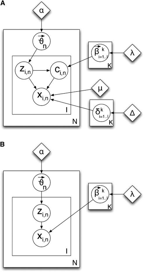where P_m() is a mutation model that can be flexibly defined on the basis of whether the genetic markers are microsatellites or single-nucleotide polymorphisms. We call this model AdMim. Figure 2A shows a graphical model representation of the overall generative scheme for AdMim, in comparison with the Adaf model underlying Structure. From Figure 2, we can clearly see that mStruct is an extended Structure model that allows copying errors.

Figure 2.—

Graphical models: the circles represent random variables and diamonds represent hyperparameters.

For simplicity of presentation, in the model described above, we assume that for a particular individual, the genetic markers at each locus are conditionally iid samples from a set of population-specific fixed-dimensional mixture of inheritance models and that the set of founder alleles (but not their frequencies) at a particular locus is the same for all ancestral populations (i.e., ≡ μ_i). We also assume that the mutation parameters for each population at any locus are independent of the alleles at that locus (i.e., ≡ ). Also, our model assumes Hardy–Weinberg equilibrium within populations. The simplifying assumptions of unlinked loci and no linkage disequilibrium between loci within populations can be easily removed by incorporating Markovian dependencies over ancestral indicators and of adjacent loci and over other parameters such as the allele frequencies in exactly the same way as in Structure. We can also introduce Markovian dependencies over mutation parameters at adjacent loci, which might be desirable to better reflect the dynamics of molecular evolution in the genome. We defer such extensions to a future article.

Mutation model

As described above, our model is applicable to almost all kinds of genetic markers by plugging in an appropriate allele mutation model (i.e., inheritance model) P_m(). We now discuss mutation models for microsatellites and SNPs.

Microsatellite mutation model:

Microsatellites are a class of tandem-repeat loci that involve a DNA unit that is 1–4 bp in length. Microsatellite DNA has significantly high mutation rates as compared to other DNA, with mutation rates as high as 10⁻³ or 10⁻⁴ (Kelly et al. 1991; Henderson and Petes 1992). The large amount of variations present in microsatellite DNA makes it ideal for differentiating founder patterns between closely related populations. Microsatellite loci have been used before DNA fingerprinting (Queller et al. 1993), before linkage analysis (Dietrich et al. 1992), and in the reconstruction of human phylogeny (Bowcock et al. 1994). By applying theoretical models of microsatellite evolution to data, questions such as time of divergence of two populations can be attempted to be addressed (Pisani et al. 2004; Zhivotovsky et al. 2004).

The choice of a suitable microsatellite mutation model is important, for both computational and interpretation purposes. Below we discuss the mutation model that we use and the biological interpretation of the parameters of the mutation model. We begin with a stepwise mutation model for microsatellites widely used in forensic analysis (Valdes et al. 1993; Lin et al. 2006).

This model defines a conditional distribution of a progeny allele b given its progenitor allele a, both of which take continuous values

(2)

where ξ is the mutation rate (probability of any mutation), and δ is the factor by which mutation decreases as distance between the two alleles increases. Although this mutation distribution is not stationary (i.e., it does not ensure allele frequencies to be constant over the generations), it is commonly used in forensic inference due to its simplicity. To some degree δ can be regarded as a parameter that controls the probability of unit-distance mutation, as can be seen from the following identity: p(b + 1 | a)/p(b | a) = δ.

In practice, the alleles for almost all microsatellites are represented by discrete counts. The two-parameter stepwise mutation model described above complicates the inference procedure. We propose a discrete microsatellite mutation model that is a simplification of Equation 2, but captures its main idea. We posit that P(b | a) ∝ δ^|b−a|. Since b ∈ [1, ∞), the normalization constant of this distribution is

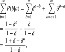which gives the mutation model as

(3)

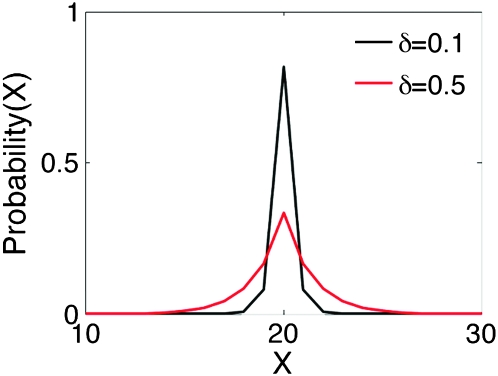
We can interpret δ as a variance parameter, the factor by which probability drops as a function of the distance between the mutated version b of the allele a. Figure 3 shows the discrete probability density function (pdf) for various values of δ.

Figure 3.—

Discrete pdf for two values of mutation parameter.

Determination of founder set at each locus:

According to our model assumptions, there can be a different number of founder alleles at each locus. This number is typically smaller than the number of alleles observed at each marker since the founder alleles are “ancestral.” To estimate the appropriate number and allele states of founders, we fit finite mixtures (of fixed size, corresponding to the desired number of ancestral alleles) of microsatellite mutation models over all the measurements at a particular marker for all individuals. We use the Bayesian information criterion (BIC) (Schwarz 1978) to determine the best number and states of founder alleles to use at each locus, since information criteria tend to favor a smaller number of founder alleles that fit the observed data well.

For each locus, we fit many different finite-sized mixtures of mutation distributions, with the size varying from 1 to the number of observed alleles at the locus. For each mixture size, the likelihood is optimized and a BIC value is computed. The number of founder alleles is chosen to be the size of the mixture that has the best (minimum) BIC value. We can do this as a pre-processing step before the actual inference or estimation procedures. This is possible since we assumed that the set of founder alleles at each locus was the same for all populations.

Choice of mutation prior:

In our model, the δ parameter, as explained above, is a population-specific parameter that controls the probability of stepwise mutations. Being a parameter that controls the variance of the mutation distribution, there is a possibility that inference on the model will encourage higher values of δ to improve the log-likelihood, in the absence of any prior distribution on δ. To avoid this situation, and to allow more meaningful and realistic results to emerge from the inference process, we impose on δ a beta prior that is biased toward smaller values of δ. The beta prior is a fixed one and is not among the parameters we estimate.

SNP mutation model:

SNPs represent the largest class of individual differences in DNA. In general, there is a well-defined correlation between the age of the mutation producing a SNP allele and the frequency of the allele. For SNPs, we use a simple pointwise mutation model, rather than more complex block models. Thus, the observations in SNP data are only binary (0/1) in nature. So, given the observed allele b, we say that the probability of it being derived from the founder allele a is given by

(4)

In this case, the mutation parameter δ is the probability that the observed allele is not identical to the founder allele, but derived from it due to a mutation.

INFERENCE AND PARAMETER ESTIMATION

For notational convenience, we ignore the diploid nature of observations in the analysis that follows. With the understanding that the analysis is carried out for an arbitrary nth individual, we drop the subscript n. Also, we overload the indicator variables z_i and c_i to be both arrays with only one element equal to 1 and the rest equal to 0, as well as scalars with a value equal to the index at which the array forms have 1's. In other words, z_i ∈ {1,…, K} or z_i ≡ [z_i,1,…, z_i,K], where , and denotes an indicator function that equals to 1 when the predicate argument is true and 0 otherwise. A similar overloading is also assumed for the c_i variables. For generalization across different types of markers, we use to denote P(x_i | c_i, z_i, μ_i, δ_i). Different mutation models can be used in AdMim by varying the form of the function f ().

The joint probability distribution of the data and the relevant variables under the AdMim model can then be written as

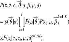The marginal likelihood of the data can be computed by summing/integrating out the latent variables:

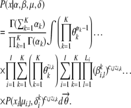However, a closed-form solution to this summation/integration is not possible, and indeed exact inference on hidden variables such as the structure vector and estimation of model parameters such as the mutation rates δ under AdMim is intractable. Pritchard et al. (2000) presented an MCMC algorithm for approximate inference for their admixture model underlying Structure. While it is straightforward to implement a similar MCMC scheme for AdMim, we choose to apply a computationally more efficient approximate inference method known as variational inference (Jordan et al. 1999).

Variational inference:

We use a mean-field approximation for performing inference on the model. This approximation method approximates an intractable joint posterior p() of all the hidden variables in the model by a product of marginal distributions , each over only a single hidden variable. The optimal parameterization of q_i() for each variable is obtained by minimizing the Kullback–Leibler divergence between the variational approximation q and the true joint posterior p. Using results from the generalized mean field theory (Xing et al. 2003), we can write the variational distributions of the latent variables in AdMim as follows:

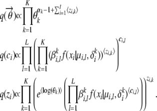In the distributions above, the “〈·〉” are used to indicate the expected values of the enclosed random variables. A close inspection of the above formulas reveals that these variational distributions have the form , q(z_i) ∼ Multinomial(ρ_i,1,…, ρ_i,K), and q(c_i) ∼ Multinomial(ξ_i,1,…, ξ_i,L), respectively, of which the parameters γ_k, ρ_i,k and ξ_i,l are given by the equations

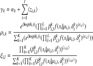and they have the properties , = ρ_i,k, and = ξ_i,l, which suggest that they can be computed via fixed point iterations. [The digamma function ψ() used above is the first derivative of the logarithm of the gamma function Γ().] It can be shown that this iteration will converge to a local optimum, similar to what happens in an EM algorithm. Empirically, a near global optimum can be obtained by multiple random restarts of the fixed point iteration. Typically, such a mean-field variational inference converges much faster than sampling (Xing et al. 2003). Upon convergence, we can easily compute an estimate of the structure vector for each individual from .

Parameter estimation:

The parameters of our model are the centroids , the mutation parameters δ, the ancestral allele frequency distributions , and the Dirichlet hyperparameter that is the prior on ancestral populations, α. For the hyperparameter estimation, we perform empirical Bayes estimation using the variational expectation maximization algorithm described in Blei et al. (2003). The variational inference described in the previous section provides us with a tractable lower bound on the log-likelihood as a function of the current values of the hyperparameters. We can thus maximize it with respect to the hyperparameters. If we alternately carry out variational inference with fixed hyperparameters, followed by a maximization of the lower bound with respect to the hyperparameters for fixed values of the variational parameters, we can get an empirical Bayes estimate of the hyperparameters. The derivation, details of which we do not show here, leads to the following iterative algorithm:

1. E-step: For each individual, find the optimizing values of the variational parameters (γ_n, ρ_n, ξ_n; n ∈ 1,…, N) using the variational updates described above.

2. M-step: Maximize the resulting variational lower bound on the likelihood with respect to the model parameters, namely α, β, μ, δ.

The two steps are repeated until the lower bound on the log-likelihood converges. The details of estimation of each hyperparameter are included in the appendix.

EXPERIMENTS AND RESULTS

We validated our model on synthetic microsatellite data sets simulated using a coalescent model to assess the performance of mStruct in terms of the accuracy and consistency of the estimated structure vectors and to test the correctness of the inference and estimation algorithms we developed. We also conducted empirical analysis using mStruct of two real data sets: the HGDP–CEPH cell line panel of microsatellite loci and the HGDP SNP data, in comparison with the Structure program (version 2.2).

Validations on coalescent simulations:

To verify the correctness of the empirical admixture estimations based on mStruct when the truth is known, we first simulated a multitude of admixture population data sets, using coalescent techniques described in Hudson (1990), under various user-specified admixing scenarios. Specifically, following Hudson (R. Hudson, personal communications), without loss of generality we simulated genealogy trees for two discrete populations of effective size 2N, which were assumed to have split from a single ancestral population, also of size 2N, at a time N generations in the past. We assumed that there was no migration between the populations after the split. These two discrete populations were joined together to form a single random-mating population. (A simulation of multiple-population admixing is possible, but tedious, and thus omitted here for simplicity.) After a single generation of random mating, samples were collected from the resulting population. Individuals, therefore, have i parents from population 1 and 2 − i parents from population 2 with probability . Every locus was simulated independently. Microsatellite mutation was modeled by a simple stepwise mutation process. The mutation parameter 4Nμ was varied over data points, with three discrete values, {8, 16, 32}, being used. Since the expected number of mutations within the populations is given by 2Nμ, the values chosen are representative of the diversity observed in real data (Pritchard et al. 2000).

For each individual, we stored the fractional contribution of population 1 to its genome. For each data set, we also stored the fractional contribution of population 1 to the entire population. To ensure that each population was well represented in the admixed population, only data sets that had roughly equal contribution from both populations were accepted (the contribution of population 1 to the resulting population was required to be in [50 − 0.01, 50 + 0.01]%). For each data point in the graph, 10 data sets were simulated using the same parameter settings for the mutation parameter. Each data set had 60 individuals from the admixed population measured at 100 loci. For each data set, 10 runs of each software (i.e., mStruct and Structure) were used to determine the run with best likelihood. The statistics used in the result were computed only on the run with the best likelihood.

We used the simulated data sets to carry out three analyses. First, we study the ability of both softwares to recover the contribution of population 1 (denoted as η) to the resulting admixed population. Next, we study how well each software is able to recover the proportion of ancestry in population 1 for each individual. Finally, we consider the problem of model selection—i.e., choosing the number of ancestral populations to provide an appropriate representation of the data.

Recovering the contribution of population 1 to the resulting population:

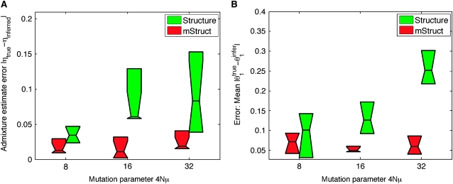
We evaluated the accuracy of the estimated η under three different conditions, one for each value of the magnitude of the mutation parameter described above. The greater the magnitude is, the more difficult the estimation of admixing coefficient η, because more discrepancy would exist between the ancestral alleles and the simulated population alleles. As a measure of error, we used the absolute difference between the true value η^true and the inferred value η^infer. The results shown in Figure 4A denote the means and quartiles of the result statistics. From Figure 4A, we can see that as the magnitude of the mutation parameter increases, the error for Structure increases. However, for mStruct, there is no significant effect of the mutation parameter on the error. mStruct also performs better than Structure over all the data points.

Figure 4.—

Recovery of individual- and population-level admixture parameters.

Recovering the contribution of population 1 to the ancestry of an individual:

We used the same data from the earlier experiment for this analysis. In this case, we used the mean of the absolute difference between the true and inferred values of the proportion of ancestry of individuals in population 1 as the measure of error. Figure 4B shows the results of this analysis. The results follow a similar trend as in the earlier experiment. For Structure, an increase in the mutation parameter causes as increase in the error, but there is no significant effect of the mutation parameter on the error for mStruct. We show the results for a particular data set with mutation parameter 4Nμ = 32 in Figure 5. Figure 5A shows the true ancestry proportion map for the sample. It shows that around half the individuals are admixed. Figure 5, B and C, shows the ancestry proportion maps inferred by Structure and mStruct, respectively. We can see that the ancestry structure recovered by mStruct is very close to the true ancestry proportions. The recovery of ancestry proportions by Structure is not very close to the truth in this case.

Figure 5.—

A comparison of the true and inferred ancestry proportions for a single example. (A) The true ancestry proportions for the sample. (B) The ancestry proportions inferred by Structure. (C) The ancestry proportions inferred by mStruct.

Model selection—choice of K:

As in Structure, our model is defined for a particular value of K, the number of ancestral populations. In general, it is not always clear what value of K must be chosen to interpret the data appropriately. We performed an experiment on the simulated data to determine the most appropriate number of ancestral populations for the data. In this case, only a single data set was used with the mutation parameter 4Nμ set to 16. For each value of K from 1 to 5, we performed 10 runs of mStruct on the data and chose the run with the best likelihood for model selection. To choose the best value of K, we used the BIC (Schwarz 1978) (that we previously used to decide the optimal number of ancestral alleles at each locus). The preferred model is the one that has the minimum value of the BIC. Table 1 shows the BIC values for the values of K. From Table 1, we can see that the model with K = 2 ancestral populations is correctly chosen as the optimal model.

TABLE 1.

Model selection for simulated data: BIC values for K from 1 to 5

K	BIC
1	6.91 × 104
2	6.87 × 104
3	6.99 × 104
4	7.12 × 104
5	7.26 × 104

The model having a smaller BIC value (K = 2 in this case) is preferred (numbers in boldface type).

Empirical analysis of real data sets:

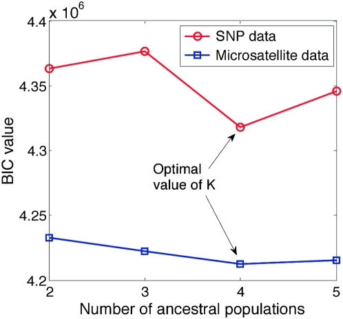
The HGDP–CEPH cell line panel (Cann et al. 2002; Cavalli-Sforza 2005) used in Rosenberg et al. (2002) contains genotype information from 1056 indviduals from 52 populations at 377 autosomal microsatellite loci, along with geographical and population labels. The HGDP SNP data (Conrad et al. 2006) contain the SNP genotypes at 2834 loci of 927 unrelated individuals that overlap with the HGDP–CEPH data. To make results for both types of data comparable, we chose the set of only those individuals present in both data sets. As in Rosenberg et al. (2002), the choice of the total number of ancestral populations can be left to the user; we tried K ranging from 2 to 5, and we applied the BIC to decide the Bayes optimal number of ancestral populations within this range to be K = 4. Below, we present the structural analysis under four ancestral populations.

Structural map from the HGDP–CEPH data:

We compare the structural maps inferred from the microsatellite data using mStruct and Structure in Figure 6. The most obvious difference between the maps produced by both programs is the degree of admixing that the individuals in the program are assigned. Structure assigns each geographical population to a distinct ancestral allele-frequency profile. This assignment is very useful for partitioning individuals into separate clusters. However, in doing so, it is unable to capture the genetic structural relationships between individuals. It offers no insights into the admixture history of populations, as mStruct does. In contrast, the structure map produced by mStruct from microsatellite data suggests that all populations share a common ancestral population as a unique extra component (represented by the magenta color in Figure 6) that characterizes their particular regional genotypes. A structure map, characterized thus by an underlying commonality in a part of the genetic ancestry, together with regional differences, clearly reveals the expansion of humans out of Africa (Hammer et al. 1998; Templeton 2002). It is in this regard that Structure and mStruct are significantly different.

Figure 6.—

Ancestry structure maps inferred from the microsatellite portion of the HGDP data set, using mStruct and Structure with four ancestral populations. The colors represent different ancestral populations.

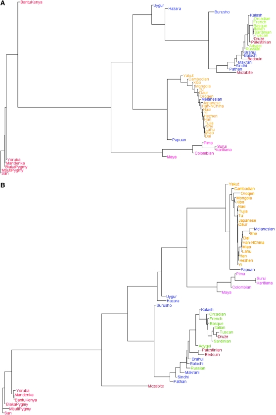
Both structure maps show that individuals having a similar population label (at regional, national, or continental levels) have similar admixture proportions. The similarity is least if two individuals come from different continents and most if two individuals are from the same region. We can therefore represent each regional population by the average of the admixture proportions of all individuals from the region. We computed the Euclidean distance between all pairs of the 52 regional populations and constructed a neighbor-joining tree from the distance matrices. Figure 7, A and B, shows the neighbor-joining trees constructed for Structure and mStruct. It is important to note that the distance measure used is not known to be a true measure of evolutionary distance. These trees have been constructed from a single instance of the distance matrix and have not been bootstrapped. Despite this, we can see that the mStruct tree agrees quite well with previously constructed phylogenetic trees for human populations (Bowcock et al. 1994). The phylogeny from mStruct appears to be more interpretable than that from Structure. In Figure 7B, we can see a tighter cluster for the African populations and that American populations diverged after Asian and European populations diverged, rather than before.

Figure 7.—

Neighbor-joining trees constructed using mStruct and Structure for the 52 regional populations in the HGDP microsatellite data. (A) Tree constructed using Structure. (B) Tree constructed using mStruct.

Analysis of the mutation spectra:

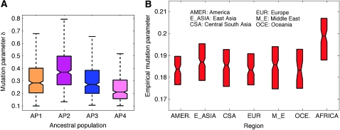
Now we report a preliminary analysis of the evolutionary dynamics reflected by the estimated mutation spectra of different ancestral populations (denoted “am-spectrum”) and of different modern geographical populations (denoted “gm-spectrum”), which is not possible by Structure. For the am-spectrum (Figure 8A), we compute the mean mutation rates over all loci and founding alleles for each ancestral population as estimated by mStruct. We estimate the gm-spectrum (Figure 8B) as follows: for every individual, a mutation parameter is computed as the per-locus number of observed alleles that are attributed to mutations, weighted by the mutation parameters corresponding to the ancestral allele chosen for that locus. This can be computed by observing the population indicator (Z) and the allele indicator (C) for each locus of the individual. We then compute the population mutation parameters by averaging mutation parameters of all individuals having the same geographical label.

Figure 8.—

Am-spectrum and Gm-spectrum inferred from the microsatellite portion of the HGDP data set, using mStruct with four ancestral populations. The colors represent different ancestral populations.

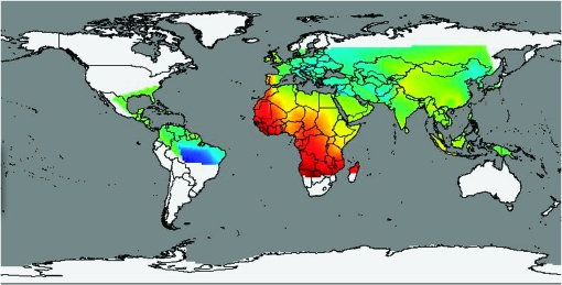
As shown in the gm-spectrum in Figure 8B, the mutation parameters for African populations are indeed higher than those of other modern populations. Since the mutation parameter reflects effects of mutation rate and population age, this indicates that they diverged earlier, a common hypothesis of human migration. Other trends in the gm-spectra also reveal interesting insights. We computed the empirical mutation parameters for each of the 52 subpopulations present in the data as we did for each continent. Since each population has an associated latitude and longitude, this allows us to set up a function that maps a geographical latitude/longitude coordinate to an empirical mutation parameter. Figure 9 shows the contour plot of this function. The mutation parameter δ in our model is a measure of variability (a combination of per generation mutation rate and age of the population). Thus, the contour plots shows us how the amount of variability changes across the world. We can see that the maximum variation is in Africa. There is a decrease in variation as we move away from central Africa. We can also see that the South American tribes have the least amount of accumulated variation. This is in qualitative agreement with the ages of different populations as predicted by the “Out of Africa” hypothesis of human migration.

Figure 9.—

Contour map of the empirical mutation parameters over the world map.

Structural map from the HGDP SNP data:

Figure 10 shows the structural maps produced by mStruct and Structure for the HGDP SNP data. We can see that the two population maps are nearly identical, which signals an inconsistency between the microsatellite and SNP mStruct results for the human data. However, there are some important caveats that must be taken into consideration. In our analysis, we consider a simplistic Bernoulli-like model of SNP mutation. While richer mutation models could potentially reduce this difficulty, there is a more significant difficulty with the analysis of SNP data. The biallelic nature of SNP markers makes it difficult to draw any inferences about the correct number of ancestral alleles at a locus. For microsatellites, this problem is considerably easier due to their multiallelic nature. As a result, mStruct is unable to obtain more information about evolutionary history from SNP markers than Structure does. As we explained earlier, mStruct is an extension of Structure that finds signals about mutations present in the data. So in the event that mStruct is unable to find any extra mutation information from the data, it is quite reasonable to expect its output to be nearly the same as that of Structure.

Figure 10.—

Ancestry structure maps inferred from the SNP portion of the HGDP data set, using mStruct and Structure with four ancestral populations.

Model selection:

As with all probabilistic models, we face a trade-off between model complexity and the log-likelihood value that the model achieves. In our case, complexity is controlled by the number of ancestral populations we pick, K. Unlike nonparametric or infinite-dimensional models (Dirichlet processes, etc.), for models of fixed dimension, it is not clear in general as to what value of K gives us the best balance between model complexity and log-likelihood. In such cases, different information criteria are often used to determine the optimal model complexity. To determine what number of ancestral populations fit the HGDP SNP and microsatellite data best, we computed BIC scores for K = 2–5 for both kinds of data separately. The results are shown in Figure 11. From the BIC curves for both SNP and microsatellite data, we can see that the curves suggest K = 4 as the best fit for the data.

Figure 11.—

Model selection with BIC score for the HGDP data with mStruct on SNP and microsatellite data.

DISCUSSION

The task of estimating the genetic contributions of ancestral populations, i.e., structural map estimation, in each modern individual, is an important problem in population genetics. Due to the relatively high rates of mutation in markers such as microsatellites and SNPs, multilocus genotype data usually harbor a large amount of variations, which allows differentiation even between populations that have close evolutionary relationships. However, to our knowledge, none of the existing methods is able to take advantage of this property to compare how marker mutation rates vary with population and locus, while at the same time exploiting such information for population structural estimation. Traditionally, population structure estimation and mutation spectrum estimation have been performed as separate tasks.

We have developed mStruct, which allows estimation of genetic contributions of ancestral populations in each modern individual in light of both population admixture and allele mutation. The variational inference algorithm that we developed allows tractable approximate inference on the model. The ancestral proportions of each individual enable representing population structure in a way that is visually easy to interpret, as well as amenable to further computational analysis.

The statistical modeling differences between mStruct and Structure provide an interesting insight into the possible reasons that lead to mStruct inferring higher levels of admixture than Structure. In Structure's representation of population, every microsatellite allele is considered to be a separate element of the population, even though they might be very similar. In the inheritance model representation, such alleles are considered to be possibly derived from a single ancestral allele. This can lead to detection of extra similarity among individuals possessing these alleles. This is probably the main reason that the inferred levels of admixture are higher in mStruct than in Structure.

Another parameter that would also affect inferred levels of admixture is the δ-parameter that determines the variance of the mutation distributions. Higher values of δ (tending to 1) lead to significantly higher levels of inferred admixture. If a strong prior is not used, the δ-values tend toward 1 in the initial few steps of the variational EM algorithm. This seems to happen due to the initial imprecise assignments for the z and c indicator variables. However, the region of high δ-values is a region of low log-likelihood in the parameter space and the EM quickly finds a local optimum that is undesirable due to the low log-likelihood of that region of the parameter space.

In conjunction with geographical location, the inferred ancestry proportions could be used to detect migrations, subpopulations, etc. Moreover, the ability to estimate population- and locus-specific mutation parameters also allows us to substantiate evolutionary dynamics claims on the basis of high/low mutation parameters in certain geographical populations or on the basis of high/low mutation parameters at certain loci in the genome. While the estimates of mutation parameters that mStruct provides are not on an absolute scale, the comparison of their relative magnitudes is certainly informative.

The mutation model we currently use is a computationally simple one. However, it lacks the ability to distinguish between the effects of per generation mutation rate and the age of the population. Under the stepwise mutation model, we can model inheritance by using a more complex but powerful model, using Bessel functions (Felsenstein 2004). This form would allow separate inference of the per generation mutation rate as well as the age of the population.

As of now, a number of possible extensions remain to the methodology we presented so far. It would be instructive to see the impact of allowing linked loci as in Falush et al. (2003). We have not yet addressed the issue of the most suitable choice of mutation process, but instead have chosen one that is reasonable and computationally tractable. It would also be interesting to combine mStruct with the nonparametric Bayesian models based on the Dirichlet processes as in programs such as Spectrum (Sohn and Xing 2007) and Structurama (Huelsenbeck and Andolfatto 2007).

In summary, current population stratification methods such as Structure ignore the effects of allele mutations, which are a significant factor in shaping allele diversity in microsatellites in human populations. In doing so, they are restricted to clustering human genetic data rather than being able to identify admixing of populations. Clustering is useful for population stratification, but a more accurate representation of events such as genome variations might cast more light on population evolutionary history. By incorporating the effect of allele mutations, the mStruct approach developed in this article represents such an attempt to gain more insight into the fine structures of genetic admixing of populations and their divergence times.

APPENDIX: DETAILS OF HYPERPARAMETER ESTIMATION

Bayes estimates of hyperparameters:

Denote the original set of hyperparameters by

(A1)

and the variational parameters for the nth individual by

(A2)

The variational lower bound to the log-likelihood for the nth individual is given by

(A3)

The subscripts indicate the nth individual. In the analysis below, we use z_.,n to denote {z_1,n,…, z_I,n} and c_.,n to represent {c_1,n,…, c_I,n}. As described earlier, we partition the variational approximation as

(A4)

So we can expand Equation 7 as

(A5)

The lower bound to the total data log-likelihood is

which, on substituting from Equation A5, becomes

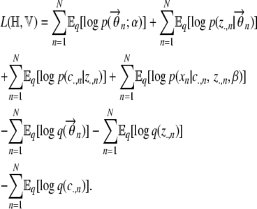(A6)

To compute and , we use the properties of a Dirichlet distribution, which is an exponential family distribution. If θ ∼ Dir(α), then the exponential family representation of p(θ; α) is given by

(A7)

So the natural parameter of the Dirichlet is η_k = α_k − 1 and the sufficient statistic is T(θ_k) = log θ_k. The log normalization factor is . For an exponential distribution, the derivative of the log normalization factor with respect to the natural parameter is equal to the expected value of the sufficient statistic. Using this fact, we get

(A8)

where ψ is the digamma function, the first derivative of the log gamma function. The remaining expectation terms in Equation A6 are expectations of multinomial parameters and hence are easy to calculate.

Simplifying each term in Equation A6, we get

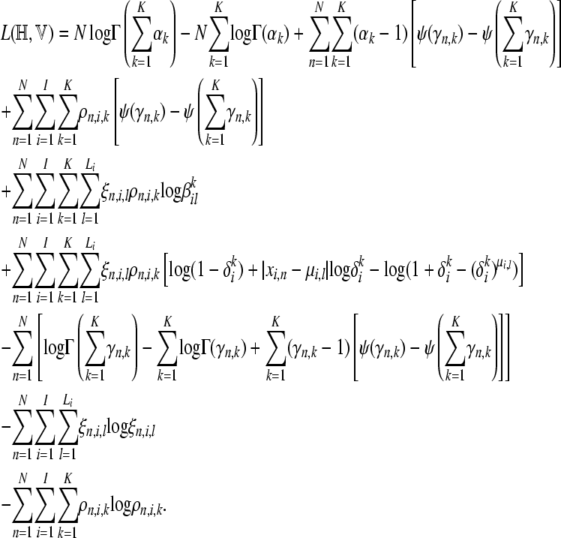(A9)

Each line in Equation A9 corresponds to an expectation term in Equation A6. In the following sections, we briefly describe how the maximum-likelihood estimates of the hyperparameters were obtained from the variational lower bound.

Estimating ancestral allele frequency profiles β:

Since β is a table of probability distributions, the values of its elements are constrained by the equality for all combinations of {i, k}. So to find the optimal values of β satisfying this constraint while maximizing the variational lower bound, we introduce Lagrange multipliers ν_i,k. The new objective function to maximize is then given by

(A10)

Maximizing this objective function gives

(A11)

We use a uniform Dirichlet prior λ on each multinomial . Under this prior, it is not difficult to show that the estimate of changes to

(A12)

Estimating the Dirichlet prior on populations α:

For estimating α we use the method described in Minka (2003). This gives a Newton–Raphson iteration for α that does not involve inversion of the Hessian and hence is reasonably fast. The log-likelihood terms involving α are

(A13)

The gradient of the log-likelihood with respect to α_k is given by

(A14)

where the digamma function used above is the first derivative of the logarithm of the gamma function.

The second derivatives, which form the Hessian, can be computed as

(A15)

(A16)

where ψ′, the trigamma function, is the derivative of the digamma function. The Hessian can then be written as

(A17)

(A18)

(A19)

where Q is a K × K matrix with elements q_j,k. As we can see from the definition, Q is a diagonal matrix. The Newton update equation we have is

(A20)

The inverse of the Hessian can be computed using the Sherman–Morris formula to be

(A21)

Therefore, we have that the update term is

(A22)

where

So the update equation for α_k is

(A23)

Estimating the ancestral alleles μ and the mutation parameters δ:

For finding the optimal values of μ and δ, we use simple gradient ascent with line search. μ-values are actually discrete variables; however, as an approximation, we assume them to be continuous in the optimization and round off the result to the nearest integer. The gradient of the variational lower bound with respect to μ_i,l is given by

(A24)

The gradient with respect to is given by

(A25)

Since the values of δ are constrained to be in [0, 1], we use the logit transformation to create a mapping from [0, 1] to . This gives us the equations

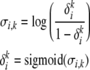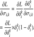We can then perform gradient ascent on each μ and δ separately and repeat this a number of times, to obtain values that increase the lower bound. To constrain values of the mutation parameter δ to allow meaningful interpretation, we use a β prior on it with a small expected value (∼0.1). We denote the prior as β(ζ₁, ζ₂).

While the gradient methods developed are useful for small data sets, they are inefficient on larger data sets and increase the time required for estimation. Hence we look at a couple of small approximations that help speed up the hyperparameter estimation. A careful look at the results that have been produced indicates that once the founder alleles have been picked initially by fitting a mixture of mutation distributions individually at each locus, the later gradient descent on makes only very minor changes in their values, if any at all. So, to improve the speed of the algorithm, we do not perform gradient descent on the founder alleles but fix them after initialization. We show below an approximation for estimating the mutation parameter δ.

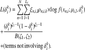
For the estimation of the mutation parameter δ, the only relevant term in the likelihood lower bound is the term

(A26)

And for the mutation distribution, we use the discrete distribution whose pdf is

(A27)

Approximation:

We assume δ to be small in Equation A27. So we can ignore the term exponential in μ in the denominator, reducing it to only (1 + δ). The expansion of (1 + δ)⁻¹ is given by

(A28)

(A29)

This gives us a lower bound to the mutation distribution of

(A30)

It is not hard to show that using this form for the mutation distribution allows a closed-form maximum-likelihood estimate for δ. This approximation gives us a lower bound to the likelihood that is not as tight as the variational lower bound. However, it offers a significant improvement in time complexity due to the existence of a closed-form solution, thus avoiding the need for slow gradient-based methods. Under this approximation, the maximum-likelihood estimate of for the microsatellite mutation model is given by

(A31)

References

- Anderson, E., and E. Thompson, 2002. A model-based method for identifying species hybrids using multilocus genetic data. Genetics 160 1217–1229. [DOI] [PMC free article] [PubMed] [Google Scholar]
- Blei, D., A. Ng and M. Jordan, 2003. Latent Dirichlet allocation. J. Mach. Learn. Res. 3 993–1022. [Google Scholar]
- Bowcock, A., A. Ruiz-Linares, J. Tomfohrde, E. Minch, J. Kidd et al., 1994. High resolution of human evolutionary trees with polymorphic microsatellites. Nature 368 455–457. [DOI] [PubMed] [Google Scholar]
- Cann, H., C. de Toma, L. Cazes, M. Legrand, V. Morel et al., 2002. A human genome diversity cell line panel. Science 296 261–262. [DOI] [PubMed] [Google Scholar]
- Cavalli-Sforza, L., 2005. The Human Genome Diversity Project: past, present and future. Nat. Rev. Genet. 6 333–340. [DOI] [PubMed] [Google Scholar]
- Conrad, D., M. Jakobsson, G. Coop, X. Wen, J. Wall et al., 2006. A worldwide survey of haplotype variation and linkage disequilibrium in the human genome. Nat. Genet. 38 1251–1260. [DOI] [PubMed] [Google Scholar]
- Corander, J., P. Waldmann and M. Sillanpaa, 2003. Bayesian analysis of genetic differentiation between populations. Genetics 163 367–374. [DOI] [PMC free article] [PubMed] [Google Scholar]
- Dietrich, W., H. Katz, S. Lincoln, H. Shin, J. Friedman et al., 1992. A genetic map of the mouse suitable for typing intraspecific crosses. Genetics 131 423–447. [DOI] [PMC free article] [PubMed] [Google Scholar]
- Erosheva, E., S. Fienberg and J. Lafferty, 2004. Mixed-membership models of scientific publications. Proc. Natl. Acad. Sci. USA 101 5220–5227. [DOI] [PMC free article] [PubMed] [Google Scholar]
- Excoffier, L., and G. Hamilton, 2003. Comment on genetic structure of human populations. Science 300 1877. [DOI] [PubMed] [Google Scholar]
- Falush, D., M. Stephens and J. Pritchard, 2003. Inference of population structure using multilocus genotype data linked loci and correlated allele frequencies. Genetics 164 1567–1587. [DOI] [PMC free article] [PubMed] [Google Scholar]
- Felsenstein, J., 2004. Inferring Phylogenies. Sinauer Associates, Sunderland, MA.
- Hammer, M. F., T. Karafet, A. Rasanayagam, E. T. Wood, T. K. Altheide et al., 1998. Out of Africa and back again: nested cladistic analysis of human y chromosome variation. Mol. Biol. Evol. 15 427–441. [DOI] [PubMed] [Google Scholar]
- Henderson, S., and T. Petes, 1992. Instability of simple sequence DNA in Saccharomyces cerevisiae. Mol. Cell. Biol. 12 2749–2757. [DOI] [PMC free article] [PubMed] [Google Scholar]
- Hudson, R., 1990. Gene genealogies and the coalescent process. Oxf. Surv. Evol. Biol. 7 1–44. [Google Scholar]
- Huelsenbeck, J., and P. Andolfatto, 2007. Inference of population structure under a Dirichlet process model. Genetics 175 1787–1802. [DOI] [PMC free article] [PubMed] [Google Scholar]
- Jordan, M., Z. Ghahramani, T. Jaakkola and L. Saul, 1999. An introduction to variational methods for graphical models. Mach. Learn. 37 183–233. [Google Scholar]
- Kelly, R., M. Gibbs, A. Collick and A. Jeffreys, 1991. Spontaneous mutation at the hypervariable mouse minisatellite locus Ms6-hm: flanking DNA sequence and analysis of germline and early somatic mutation events. Proc. Biol. Sci. 245 235–245. [DOI] [PubMed] [Google Scholar]
- Lin, T., E. Myers and E. Xing, 2006. Interpreting anonymous DNA samples from mass disasters–probabilistic forensic inference using genetic markers. Bioinformatics 22 e298. [DOI] [PubMed] [Google Scholar]
- Minka, T., 2003. Estimating a Dirichlet distribution. Technical Report. Carnegie Mellon University, Pittsburgh.
- Patterson, N., A. Price and D. Reich, 2006. Population structure and eigenanalysis. PLoS Genet. 2 e190. [DOI] [PMC free article] [PubMed] [Google Scholar]
- Pella, J., and M. Masuda, 2006. The Gibbs and split-merge sampler for population mixture analysis from genetic data with incomplete baselines. Can. J. Fish. Aquat. Sci. 63 576–596. [Google Scholar]
- Pisani, D., L. Poling, M. Lyons-Weiler and S. Hedges, 2004. The colonization of land by animals: molecular phylogeny and divergence times among arthropods. BMC Biol. 2: 1. [DOI] [PMC free article] [PubMed]
- Pritchard, J., M. Stephens and P. Donnelly, 2000. Inference of population structure using multilocus genotype data. Genetics 155 945–959. [DOI] [PMC free article] [PubMed] [Google Scholar]
- Queller, D., J. Strassmann and C. Hughes, 1993. Microsatellites and kinship. Trends Ecol. Evol. 8 285–288. [DOI] [PubMed] [Google Scholar]
- Roeder, K., M. Escoar, J. Kadane and I. Balazs, 1998. Measuring heterogeneity in forensic databases using hierarchical Bayes models. Biometrika 85 269. [Google Scholar]
- Rosenberg, N., J. Pritchard, J. Weber, H. Cann, K. Kidd et al., 2002. Genetic structure of human populations. Science 298 2381–2385. [DOI] [PubMed] [Google Scholar]
- Schwarz, G., 1978. Estimating the dimension of a model. Ann. Stat. 6 461–464. [Google Scholar]
- Sohn, K., and E. Xing, 2007. Spectrum: joint Bayesian inference of population structure and recombination events. Bioinformatics 23 i479–i489. [DOI] [PubMed] [Google Scholar]
- Templeton, A., 2002. Out of Africa again and again. Nature 416 45–51. [DOI] [PubMed] [Google Scholar]
- Valdes, A., M. Slatkin and N. Freimer, 1993. Allele frequencies at microsatellite loci: the stepwise mutation model revisited. Genetics 133 737–749. [DOI] [PMC free article] [PubMed] [Google Scholar]
- Xing, E., M. Jordan and S. Russell, 2003. A generalized mean field algorithm for variational inference in exponential families, pp. 583–591 in Uncertainty in Artificial Intelligence (UAI2003). Morgan Kaufmann Publishers.
- Zhivotovsky, L., P. Underhill, C. Cinnioglu, M. Kayser, B. Morar et al., 2004. The effective mutation rate at Y chromosome short tandem repeats, with application to human population-divergence time. Am. J. Hum. Genet. 74 50–61. [DOI] [PMC free article] [PubMed] [Google Scholar]