

Abstract
The purpose of this prospective study was to compare a new isotropic three-dimensional (3D) fast spin-echo (FSE) pulse sequence with parallel imaging and extended echo train acquisition (3D-FSE-Cube) with a conventional two-dimensional (2D) FSE sequence for magnetic resonance (MR) imaging of the ankle. After institutional review board approval and informed consent were obtained and in accordance with HIPAA privacy guidelines, MR imaging was performed in the ankles of 10 healthy volunteers (four men, six women; age range, 25–41 years). Imaging with the 3D-FSE-Cube sequence was performed at 3.0 T by using both one-dimensional– and 2D-accelerated autocalibrated parallel imaging to decrease imaging time. Signal-to-noise ratio (SNR) and contrast-to-noise ratio (CNR) with 3D-FSE-Cube were compared with those of the standard 2D FSE sequence. Cartilage, muscle, and fluid SNRs were significantly higher with the 3D-FSE-Cube sequence (P < .01 for all). Fluid-cartilage CNR was similar for both techniques. The two sequences were also compared for overall image quality, blurring, and artifacts. No significant difference for overall image quality and artifacts was demonstrated between the 2D FSE and 3D-FSE-Cube sequences, although the section thickness in 3D-FSE-Cube imaging was much thinner (0.6 mm). However, blurring was significantly greater on the 3D-FSE-Cube images (P < .04). The 3D-FSE-Cube sequence with isotropic resolution is a promising new MR imaging sequence for viewing complex joint anatomy.
© RSNA, 2008
The ankle is the second most common site of injury in athletes after the knee, and ligamentous sprains are the most common sports-related injury (1). Long-term sequelae can include chronic ankle instability, ankle impingement, and eventual osteoarthritis (2). With its multiplanar imaging capabilities and high-spatial-resolution imaging of soft-tissue structures, magnetic resonance (MR) imaging is ideal for evaluating ligamentous integrity, tendon disease, and osteochondral injury in the ankle (3–10).
Three-tesla MR imaging is increasingly being used for evaluation of musculoskeletal disease (11–14). MR imaging of the ankle traditionally involves the use of multiple two-dimensional (2D) multisection acquisitions to evaluate internal derangements. However, 2D fast spin-echo (FSE) imaging has limitations in examination of the ankle, as the voxels produced are not isotropic and the relatively thick sections compared with the in-plane resolution can lead to partial volume artifacts. The anisotropic nature of the voxels also renders them unsuitable for reformations in other imaging planes.
The articular cartilage in the ankle is relatively thin, varying from 1.35 to 2.69 mm in thickness over the talus (15); therefore, the thinner section thickness images that can be obtained at 3.0 T can lead to improved diagnostic accuracy for osteochondral lesions in the ankle (14). However, the tibiotalar joint also has a complex curved surface, which can make accurate evaluation of osteochondral disease challenging. The ability to reformat the images and interrogate the articular surface in any plane may help improve visualization of cartilage defects. In addition, the numerous ligaments surrounding the ankle are oriented in different planes, making evaluation of the ligamentous structures in any one imaging plane difficult. The tendons around the ankle also run in different imaging planes as they traverse the ankle joint. Therefore, a pulse sequence that provides the ability to reformat images in multiple planes with high spatial resolution would be well suited for visualizing this complex joint anatomy.
A number of three-dimensional (3D) imaging sequences have been used to evaluate the ankle, including 3D fat-suppressed gradient-echo imaging (16,17), 3D multishot echo-planar imaging (16), and fast imaging with steady-state precession (18). The utility of 3D FSE sequences has already been established in the evaluation of intracranial structures (19,20), and, more recently, a 3D turbo spin-echo sequence was used to image the spine, pelvis, and extremities (21). The researchers in the latter study concluded that an optimized 3D sequence with isotropic imaging and high spatial resolution would be helpful in clinical practice for evaluating body parts with complex regional anatomy.
Given the large volume of data contained in an isotropic high-spatial-resolution 3D data set and the relatively long repetition times required for proton-density and T2-weighted FSE sequences, imaging time for 3D acquisitions of these types of pulse sequences would be prohibitive but for a number of recent advances. First, modulating the flip angles of the refocusing radiofrequency train enables very long readout trains to be acquired with minimal blurring (22–24). Second, parallel imaging in both phase-encoding directions (25,26) and partial Fourier acquisition (27) can greatly reduce the number of phase encodes required to encode a large 3D data set. Previously, an earlier version of flip angle modulation (23) and one-dimensional (1D)-accelerated autocalibrating parallel imaging (26,28) was reported for application to knee imaging (22). Here, we investigate the use of the new 3D-FSE-Cube sequence, which combines a more recent flip angle algorithm to determine the set of refocusing flip angles appropriate for a long echo train readout (22) with 2D-accelerated autocalibrating parallel imaging (29) for imaging of the ankle. The improved acquisition efficiency of this sequence enables isotropic acquisition, allowing the data to be reformatted in arbitrary planes, which is ideal for imaging complex anatomy such as that found around the ankle.
The purpose of our study was to compare the newly developed 3D-FSE-Cube sequence with a conventional 2D FSE sequence commonly used in clinical practice for MR imaging of the ankle.
MATERIALS AND METHODS
Volunteers and Imaging
After institutional review board approval and informed consent were obtained and in accordance with Health Insurance Portability and Accountability Act privacy guidelines, MR imaging was performed in the ankles of 10 healthy volunteers (mean age, 36 years; age range, 25–41 years): four men (mean age, 38 years; age range, 35–41 years) and six women (mean age, 35 years; age range, 25–40 years). All images were acquired between October 30, 2006, and November 24, 2006, with a 3.0-T MR imaging unit (Signa Excite HDx; GE Healthcare, Milwaukee, Wis) equipped with high-performance gradients (amplitude, 40 mT/m; slew rate, 150 mT/m/msec) by using an eight-channel head coil. All images were acquired with and without fat suppression. The authors who are not employees of GE Healthcare had control of inclusion of any data and information that might present a conflict of interest for those authors who are employees of GE Healthcare.
Imaging with 3D-FSE-Cube was performed with the following parameters: repetition time msec/echo time msec, 3000/35; matrix, 256 × 256; field of view, 15 cm; section thickness, 0.6 mm; and receiver bandwidth, ±31.25 kHz—resulting in an isotropic resolution of 0.6 mm. Partial Fourier acquisition and 1D-accelerated parallel imaging reduced the imaging time by a factor of 3.4, enabling an echo train of 78 to encode 256 lines. To cover the entire ankle, 132 sections were acquired in just 6 minutes 40 seconds. Two-dimensional acceleration was also used (acceleration factor, 4.5) with the same parameters and resulted in the acquisition of 132 sagittal sections in 5 minutes. Images were acquired both with and without fat saturation. Autocalibrating Reconstruction for Cartesian sampling parallel imaging reconstruction was performed online by using host-based prototype software, and reconstructed images were transferred to the imaging unit database.
Sagittal 2D FSE images for comparison with reformats of the 3D data were acquired in the sagittal and axial planes with the following parameters: 3000/35; matrix, 256 × 256; field of view, 15 cm; section thickness, 2 mm with a 0.5-mm gap; number of acquisitions, three; echo train length, eight; bandwidth, ±31.25 kHz; and imaging time, 5 minutes.
Image Evaluation
Signal intensity from cartilage, muscle, and synovial fluid and noise were measured in all patients in regions of interest (ROIs) in the subtalar joint cartilage, soleus muscle, and fluid in the posterior subtalar recess. Measurements were performed by a single radiologist (G.E.G., with 10 years of experience in interpretation of MR images of the ankle). The circular ROI for cartilage and fluid measurements was 3 mm in diameter. The circular ROI for muscle and noise measurements was 9 mm in diameter. The standard deviation of the noise was measured in a single ROI placed anterior to the tibiotalar joint in an area where there was no phase ghosting (phase-encoding direction, anterior to posterior). Signal-to-noise ratios (SNRs) for cartilage, muscle, and joint fluid were estimated by dividing the signal intensity level by the standard deviation of the noise. The fluid-cartilage contrast-to-noise ratio was calculated by subtracting the cartilage SNR from the fluid SNR.
Axial reformats of the isotropic 3D-FSE-Cube images were created by using software (Osirix; http://www.osirix.com/) and were compared with 2D FSE images acquired in the axial plane. Images obtained with the 3D-FSE-Cube sequence were also reformatted in multiple arbitrary imaging planes to best demonstrate the ankle ligaments, tendons, and articular cartilage of the tibiotalar and subtalar joints.
A central sagittal section through the tibiotalar joint was selected from among the 2D FSE images for each patient and was compared with a comparable section from the 3D-FSE-Cube acquisition. Similarly, an axial 2D FSE image at the level of the anterior talofibular ligament in each patient was compared with an equivalent axial reformatted 3D-FSE-Cube image. The paired images were then randomized and assessed for overall image quality, blurring, and artifact by three musculoskeletal radiologists (K.J.S., with 10 years, G.E.G., with 10 years, and C.F.B., with 14 years of musculoskeletal radiology experience) who were blinded as to which image had been obtained with which sequence. The radiologists graded the images on a five-point scale from −2 to +2, where a score of −2 indicated that image A was much better than image B; a score of −1, that image A was somewhat better than image B; a score of 0, that there was no difference between the two images; a score of +1, that image B was somewhat better than image A; and a score of +2, that image B was much better than image A.
Statistical Analysis
Statistical analysis was performed by using software (Excel, version 11.1.1; Microsoft, Redmond, Wash). The 3D-FSE-Cube and 2D FSE sequences were compared with respect to SNR and cartilage-fluid contrast-to-noise ratio by using a paired sample t test. P < .05 was considered to indicate a significant difference.
The ratings of the three readers for overall image quality, blurring, and artifacts on the axial and sagittal MR images in each of the 10 volunteers were then compared and analyzed by using a two-tailed paired Wilcoxon test and software (Stata, release 9.2; Stata, College Station, Tex).
RESULTS
Cartilage SNR was significantly higher with 3D-FSE-Cube with 1D acceleration and 0.6-mm isotropic resolution (mean, 25 ± 3 [standard error of the mean]) than with 2D FSE (19 ± 5, P = .007). Muscle SNR with 3D-FSE-Cube with 1D acceleration (29 ± 9) was also significantly higher than that with 2D FSE (14 ± 3, P = .0004). Additionally, fluid SNR was higher with 3D-FSE-Cube with 1D acceleration (76 ± 7) than with 2D FSE (67 ± 13, P = .0036) (Fig 1).
Figure 1:

Bar graph shows comparison of SNRs in cartilage, muscle, and fluid between 1D- and 2D-accelerated 3D-FSE-Cube MR imaging (3000/35) and 2D FSE MR imaging (3000/35). Images acquired with 1D-accelerated 3D-FSE-Cube had significantly higher SNR in all three tissues (* = P < .05) despite much thinner sections. The SNRs for all three tissues were similar for 2D accelerated 3D-FSE-Cube and 2D FSE (P > .1).
Use of the 2D-accelerated parallel imaging technique instead of 1D acceleration reduced the imaging time substantially, from 6 minutes 40 seconds to 5 minutes. This was the same imaging time as that with the 2D FSE sequence. Cartilage, muscle, and fluid SNRs with 3D-FSE-Cube with 2D acceleration and 0.6-mm isotropic resolution were not significantly different from those with 2D FSE (P = .0600 for cartilage, P = .239 for muscle, P = .340 for fluid) (Fig 1).
Fluid-cartilage contrast-to-noise ratio was similar for 2D FSE (48 ± 9) and 3D-FSE-Cube with 1D acceleration (51 ± 5, P = .194) and 2D acceleration (43 ± 3, P = .720). Cartilage signal intensity in 2D FSE was likely lower owing to magnetization transfer effects from the 2D acquisition (30,31). Contrast between fluid and articular cartilage was seen with both methods, with high fluid signal intensity on both 2D FSE and 3D-FSE-Cube images. Image quality was very similar for the 3D-FSE-Cube images acquired with either 1D or 2D acceleration (Fig 2).
Figure 2a:
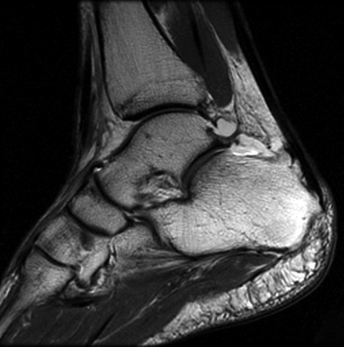
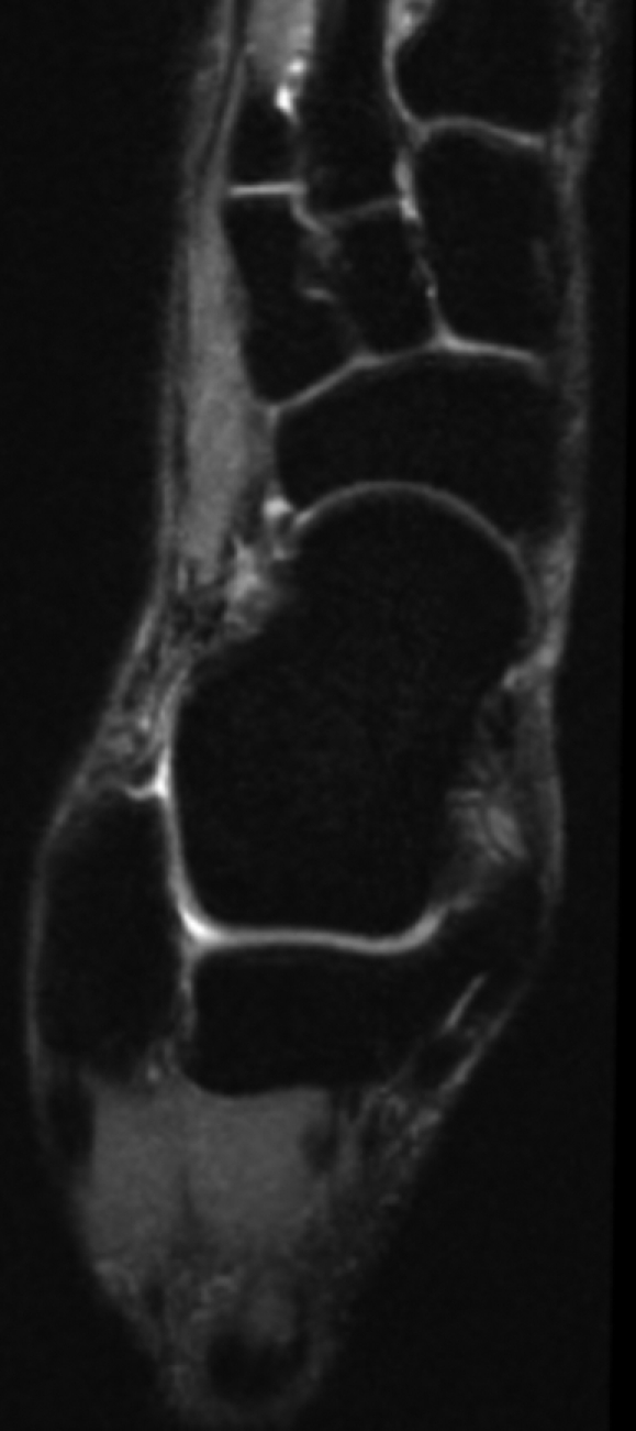
(a) Sagittal 2D FSE MR image (2-mm section thickness), (b) sagittal 3D-FSE-Cube with 1D acceleration MR image (0.6-mm section thickness), and (c) sagittal 3D-FSE-Cube with 2D acceleration MR image (0.6-mm section thickness) in healthy volunteer. Fluid is of high signal intensity in comparison to the articular cartilage.
Figure 2b:
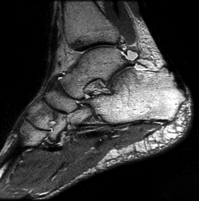
(a) Sagittal 2D FSE MR image (2-mm section thickness), (b) sagittal 3D-FSE-Cube with 1D acceleration MR image (0.6-mm section thickness), and (c) sagittal 3D-FSE-Cube with 2D acceleration MR image (0.6-mm section thickness) in healthy volunteer. Fluid is of high signal intensity in comparison to the articular cartilage.
Figure 2c:
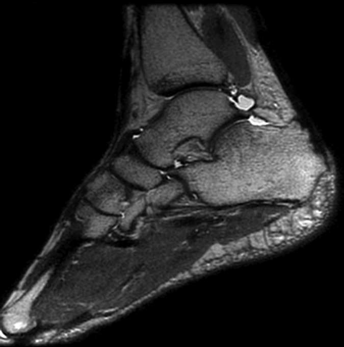
(a) Sagittal 2D FSE MR image (2-mm section thickness), (b) sagittal 3D-FSE-Cube with 1D acceleration MR image (0.6-mm section thickness), and (c) sagittal 3D-FSE-Cube with 2D acceleration MR image (0.6-mm section thickness) in healthy volunteer. Fluid is of high signal intensity in comparison to the articular cartilage.
The 2D FSE and 3D-FSE-Cube images were assessed for overall image quality, blurring, and artifacts by three readers. No significant difference was seen between overall image quality for the 2D FSE and 3D-FSE-Cube images for either axial (P < .4795) or sagittal (P < .1573) images. A significant difference between the 2D FSE and 3D-FSE-Cube sequences was demonstrated for blurring on both axial (P < .00001) and sagittal (P < .0325) images. Blurring was more pronounced on the 3D-FSE-Cube images, most likely because of the greater T2 decay during the long echo train. No statistically significant difference between the 2D FSE and 3D-FSE-Cube sequences was demonstrated for artifacts on either the axial or sagittal images (P > .99).
The 3D-FSE-Cube sequence was performed both with and without fat suppression. Fat suppression was uniform for all sequences, with no excessive blurring on the 3D-FSE-Cube images (Fig 3). The big advantage of 3D-FSE-Cube was the ability to reformat images in arbitrary planes. Reformations of the 3D-FSE-Cube images were similar to the directly acquired 2D FSE data, except that the 3D-FSE-Cube sections were much thinner. Images acquired with the 3D-FSE-Cube sequence were reformatted in multiple oblique imaging planes to optimally depict the ankle ligaments (Fig 4), the complex course of the tendons around the ankle (Figs 5, 6), and the articular cartilage of the tibiotalar and subtalar joints (Fig 7). Compared with images acquired directly in the reformation plane with 2D FSE, the reformatted 3D-FSE-Cube images were similar in quality and depiction of anatomy, only with much thinner sections. An advantage of 3D-FSE-Cube is the ability to average sections, so that both source and reformatted images can be displayed at any multiple of the 0.6-mm section thickness. Fat suppression was excellent with both 2D FSE and 3D-FSE-Cube.
Figure 3a:
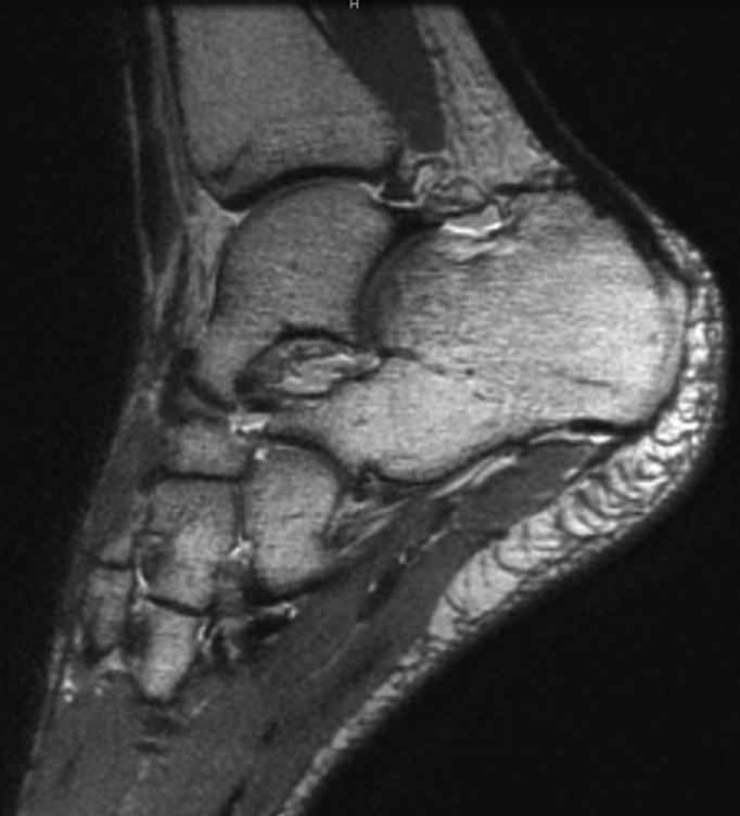
(a) Sagittal 0.6-mm 3D-FSE-Cube MR image obtained with 1D acceleration and (b) sagittal 0.6-mm 3D-FSE-Cube MR image obtained with 1D acceleration with fat saturation. There is no substantial blurring on either image.
Figure 3b:
(a) Sagittal 0.6-mm 3D-FSE-Cube MR image obtained with 1D acceleration and (b) sagittal 0.6-mm 3D-FSE-Cube MR image obtained with 1D acceleration with fat saturation. There is no substantial blurring on either image.
Figure 4a:
(a–c) Axial oblique 3D-FSE-Cube MR images obtained with 1D acceleration in differing obliquities show anterior talofibular ligament (arrow in a). (b) By tilting the axial image a little more posteriorly, it is possible to see both the anterior (arrow) and posterior (arrowhead) talofibular ligaments on the same image. (c) Tilting the axial plane more posteriorly still allows the calcaneofibular ligament (arrows) to be seen in its entirety. (d) Sagittal 3D-FSE-Cube MR image depicts planes of a (A), b (B), and c (C).
Figure 4b:
(a–c) Axial oblique 3D-FSE-Cube MR images obtained with 1D acceleration in differing obliquities show anterior talofibular ligament (arrow in a). (b) By tilting the axial image a little more posteriorly, it is possible to see both the anterior (arrow) and posterior (arrowhead) talofibular ligaments on the same image. (c) Tilting the axial plane more posteriorly still allows the calcaneofibular ligament (arrows) to be seen in its entirety. (d) Sagittal 3D-FSE-Cube MR image depicts planes of a (A), b (B), and c (C).
Figure 4c:
(a–c) Axial oblique 3D-FSE-Cube MR images obtained with 1D acceleration in differing obliquities show anterior talofibular ligament (arrow in a). (b) By tilting the axial image a little more posteriorly, it is possible to see both the anterior (arrow) and posterior (arrowhead) talofibular ligaments on the same image. (c) Tilting the axial plane more posteriorly still allows the calcaneofibular ligament (arrows) to be seen in its entirety. (d) Sagittal 3D-FSE-Cube MR image depicts planes of a (A), b (B), and c (C).
Figure 4d:
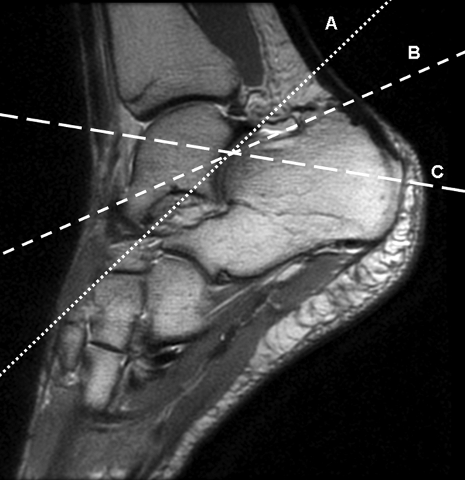
(a–c) Axial oblique 3D-FSE-Cube MR images obtained with 1D acceleration in differing obliquities show anterior talofibular ligament (arrow in a). (b) By tilting the axial image a little more posteriorly, it is possible to see both the anterior (arrow) and posterior (arrowhead) talofibular ligaments on the same image. (c) Tilting the axial plane more posteriorly still allows the calcaneofibular ligament (arrows) to be seen in its entirety. (d) Sagittal 3D-FSE-Cube MR image depicts planes of a (A), b (B), and c (C).
Figure 5a:
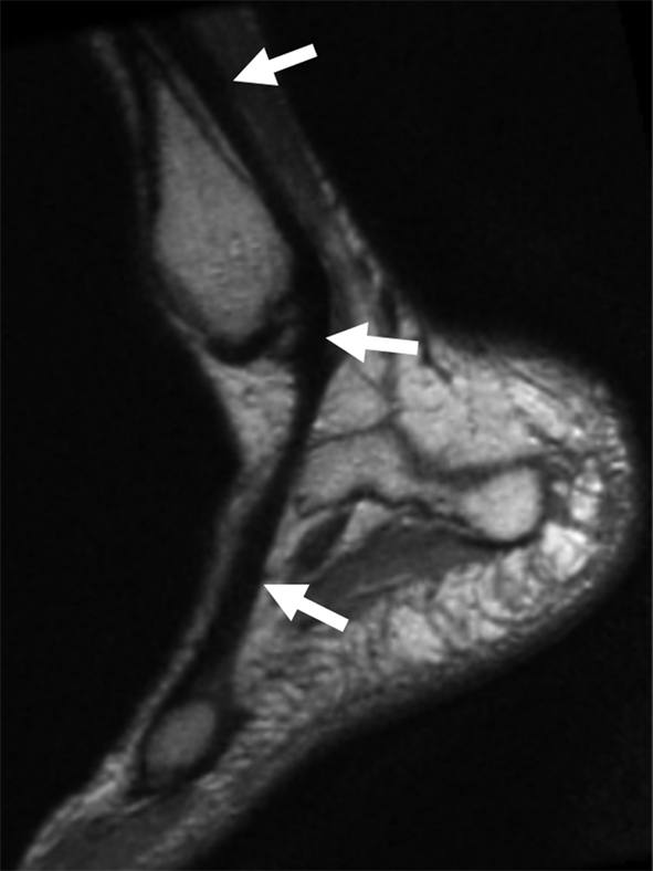
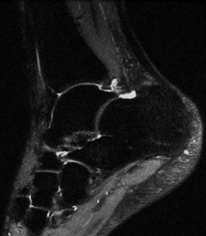
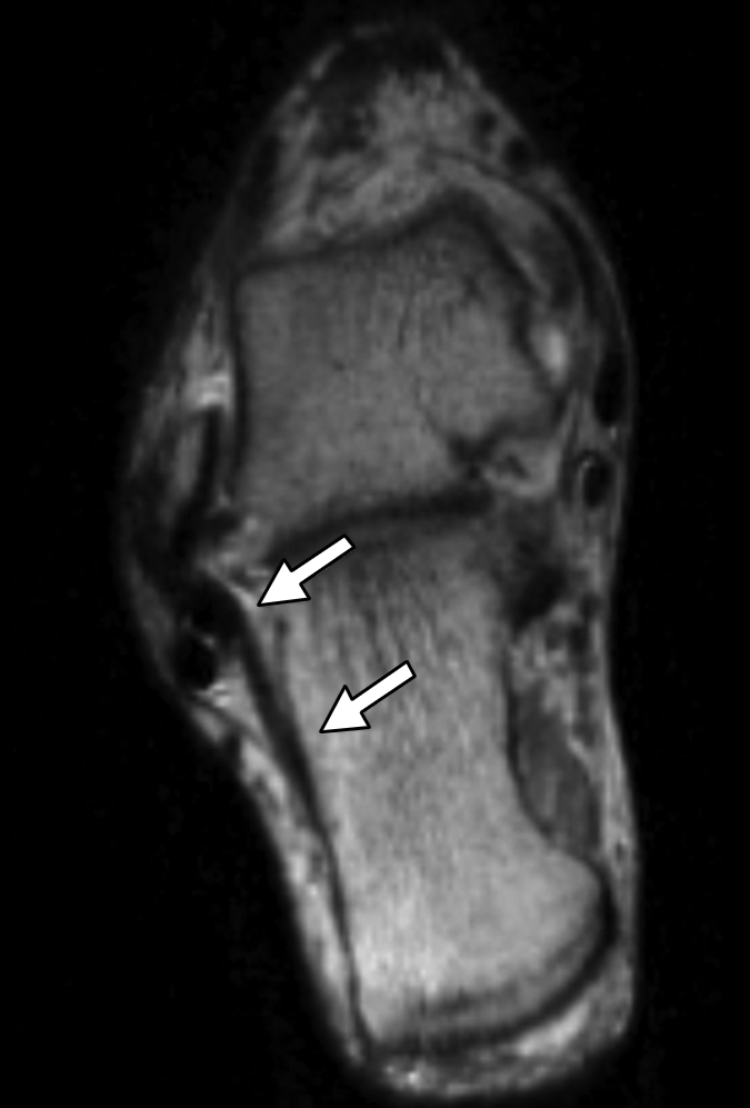
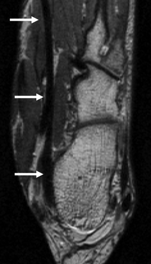
(a, b) Sagittal oblique and (c) axial oblique 3D-FSE-Cube reformatted MR images show the course of the peroneal tendons. (a) The peroneus brevis tendon (arrows) grooves the posterior surface of the lateral malleolus to insert into the base of the fifth metatarsal. (b) The peroneus longus tendon (solid arrows) passes behind the lateral malleolus, inferior to the peroneal tubercle of the calcaneus (open arrow), to the undersurface of the cuboid bone. (c) The peroneus longus tendon (arrows) passes in a groove underneath the cuboid bone to insert into the base of the first metatarsal.
Figure 5b:
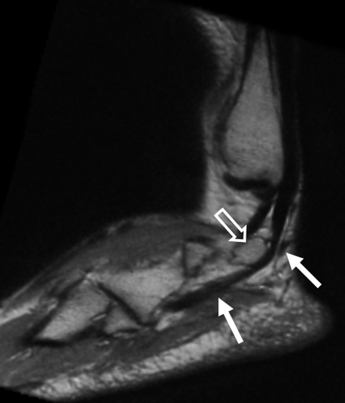
(a, b) Sagittal oblique and (c) axial oblique 3D-FSE-Cube reformatted MR images show the course of the peroneal tendons. (a) The peroneus brevis tendon (arrows) grooves the posterior surface of the lateral malleolus to insert into the base of the fifth metatarsal. (b) The peroneus longus tendon (solid arrows) passes behind the lateral malleolus, inferior to the peroneal tubercle of the calcaneus (open arrow), to the undersurface of the cuboid bone. (c) The peroneus longus tendon (arrows) passes in a groove underneath the cuboid bone to insert into the base of the first metatarsal.
Figure 5c:
(a, b) Sagittal oblique and (c) axial oblique 3D-FSE-Cube reformatted MR images show the course of the peroneal tendons. (a) The peroneus brevis tendon (arrows) grooves the posterior surface of the lateral malleolus to insert into the base of the fifth metatarsal. (b) The peroneus longus tendon (solid arrows) passes behind the lateral malleolus, inferior to the peroneal tubercle of the calcaneus (open arrow), to the undersurface of the cuboid bone. (c) The peroneus longus tendon (arrows) passes in a groove underneath the cuboid bone to insert into the base of the first metatarsal.
Figure 6a:

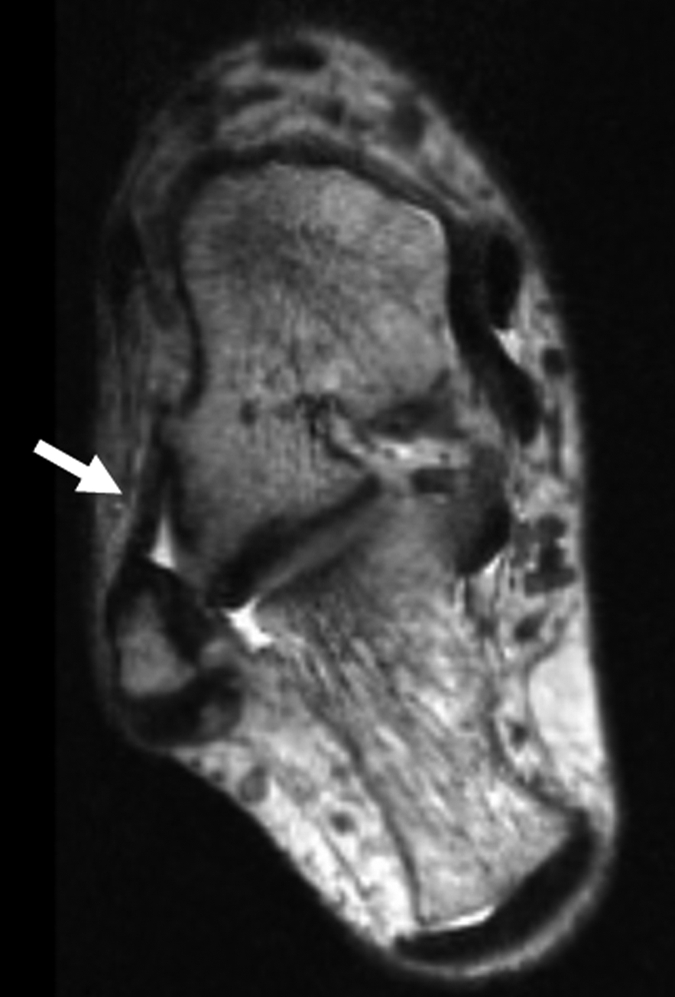
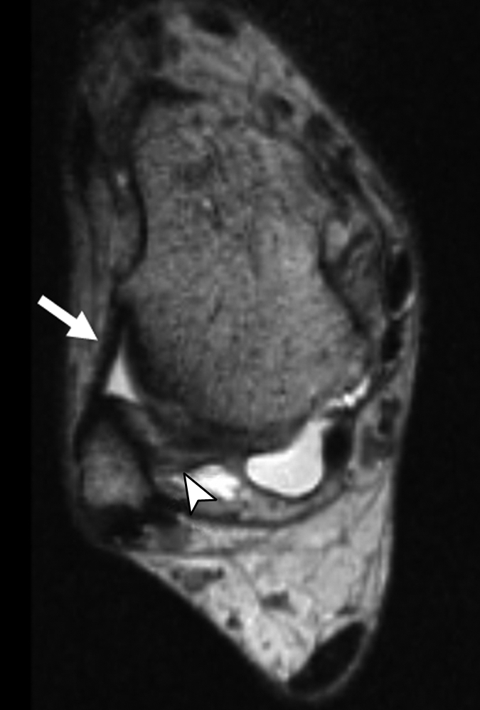
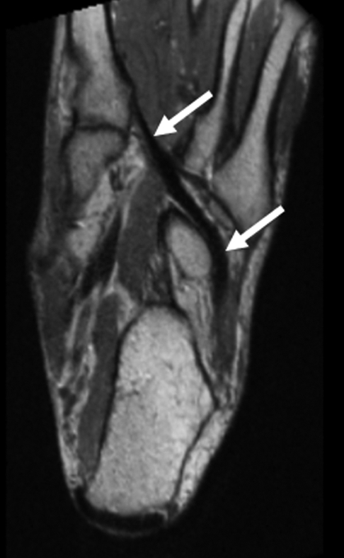
(a) Sagittal oblique and (b) axial oblique 3D-FSE-Cube reformatted MR images of left ankle show the flexor hallucis tendon (arrows) grooving the undersurface of the sustentaculum tali to pass toward the hallux (not included in the field of view). A = anterior, F = foot, H = head, P = posterior.
Figure 6b:
(a) Sagittal oblique and (b) axial oblique 3D-FSE-Cube reformatted MR images of left ankle show the flexor hallucis tendon (arrows) grooving the undersurface of the sustentaculum tali to pass toward the hallux (not included in the field of view). A = anterior, F = foot, H = head, P = posterior.
Figure 7a:
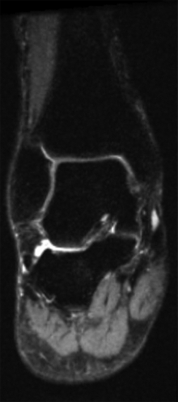
(a) Coronal and (b) sagittal 3D-FSE-Cube reformatted MR images with fat saturation show the articular cartilage of the tibial plafond and subtalar joints. However, 3D-FSE-Cube data can be reformatted in multiple imaging planes to view cartilage over areas of bone that are not easily seen with conventional orthogonal sequences. (c) Sagittal oblique 3D-FSE-Cube MR image shows cartilage over the lateral talar dome, where cartilage is usually thickest. (d) Axial oblique 3D-FSE-Cube MR image shows articular cartilage over the anterior tibiotalar joint, as well as in the intertarsal and tarsometatarsal joints.
Figure 7b:
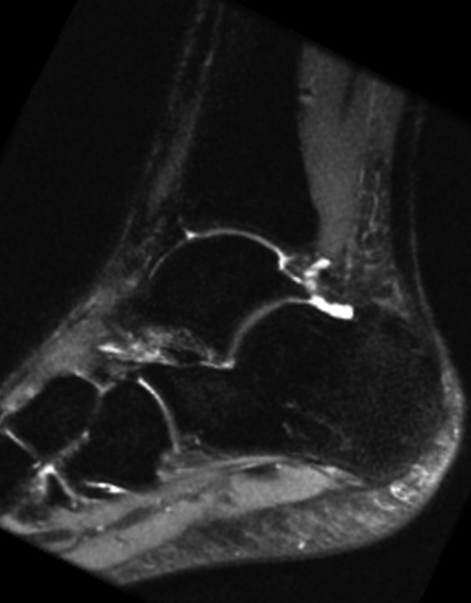
(a) Coronal and (b) sagittal 3D-FSE-Cube reformatted MR images with fat saturation show the articular cartilage of the tibial plafond and subtalar joints. However, 3D-FSE-Cube data can be reformatted in multiple imaging planes to view cartilage over areas of bone that are not easily seen with conventional orthogonal sequences. (c) Sagittal oblique 3D-FSE-Cube MR image shows cartilage over the lateral talar dome, where cartilage is usually thickest. (d) Axial oblique 3D-FSE-Cube MR image shows articular cartilage over the anterior tibiotalar joint, as well as in the intertarsal and tarsometatarsal joints.
Figure 7c:
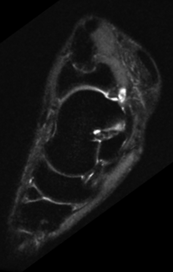
(a) Coronal and (b) sagittal 3D-FSE-Cube reformatted MR images with fat saturation show the articular cartilage of the tibial plafond and subtalar joints. However, 3D-FSE-Cube data can be reformatted in multiple imaging planes to view cartilage over areas of bone that are not easily seen with conventional orthogonal sequences. (c) Sagittal oblique 3D-FSE-Cube MR image shows cartilage over the lateral talar dome, where cartilage is usually thickest. (d) Axial oblique 3D-FSE-Cube MR image shows articular cartilage over the anterior tibiotalar joint, as well as in the intertarsal and tarsometatarsal joints.
Figure 7d:
(a) Coronal and (b) sagittal 3D-FSE-Cube reformatted MR images with fat saturation show the articular cartilage of the tibial plafond and subtalar joints. However, 3D-FSE-Cube data can be reformatted in multiple imaging planes to view cartilage over areas of bone that are not easily seen with conventional orthogonal sequences. (c) Sagittal oblique 3D-FSE-Cube MR image shows cartilage over the lateral talar dome, where cartilage is usually thickest. (d) Axial oblique 3D-FSE-Cube MR image shows articular cartilage over the anterior tibiotalar joint, as well as in the intertarsal and tarsometatarsal joints.
DISCUSSION
Traditional ankle MR imaging protocols usually include multiple 2D FSE sequences acquired in orthogonal planes. Parallel imaging with generalized autocalibrating reconstruction algorithms (eg, generalized autocalibrating partially parallel acquisitions, or GRAPPA) has been used more recently to decrease the imaging time of conventional pulse sequences (32,33). In the case of 3D-FSE-Cube, parallel imaging permits the imaging time to be in an acceptable range (5–8 minutes). Because the imaging time in parallel imaging is reduced, the SNR in parallel imaging is proportional to the SNR of a nonaccelerated image divided by the square root of the acceleration factor. Despite the relative reduction in SNR due to parallel imaging, 3D-FSE-Cube had comparable or better SNR than 2D FSE in our study.
The 3D-FSE-Cube with half-Fourier acquisition and 2D-accelerated autocalibrating parallel imaging technique provides high-quality isotropic images of the ankle with similar contrast to those obtained with 2D FSE, although there is slightly increased blurring on the 3D-FSE-Cube images, likely due to T2 decay during the long echo train. However, the blurring did not decrease the overall image quality, which was not significantly different between the two sequences. On all 3D-FSE-Cube images, parallel imaging artifacts were minimal because of the robust autocalibrating nature of the Autocalibrating Reconstruction for Cartesian sampling technique. Isotropic data from 3D-FSE-Cube imaging enable reformations in arbitrary planes, optimizing visualization of the ligaments and the complex course of the tendons around the ankle.
The imaging time for the 3D-FSE-Cube sequence with 1D acceleration techniques is slightly longer than for conventional 2D FSE sequences. However, the 3D-FSE-Cube sequence makes multiple 2D acquisitions unnecessary, as images can subsequently be reformatted in multiple orthogonal planes. Image quality was generally comparable for the 3D-FSE-Cube sequence with 2D acceleration, which can be performed in considerably less time than the 1D acceleration, making this sequence well suited for patients in pain, pediatric patients who are unable to stay still for long, and patients with claustrophobia who are able to tolerate lying in the magnet bore only for short periods of time. The specific absorption rate of 3D-FSE-Cube was well within Food and Drug Administration limits for both the 1D and the 2D acceleration methods. The section thickness in 3D-FSE-Cube imaging is also approximately three times less than that in 2D FSE imaging, thereby decreasing partial-volume artifacts and further improving depiction of anatomy.
Cartilage and muscle SNRs were lower for the 2D FSE sequence than for the 3D-FSE-Cube sequence with 1D acceleration. One explanation is the inherent higher SNR in 3D acquisitions. There may also have been a small magnetization transfer effect due to the long echo train in 3D-FSE-Cube imaging. The magnetization transfer effect decreases the signal in cartilage and muscle in 2D FSE acquisitions because of the effect on out-of-section spins with section selection pulses (30,31).
Our study was limited in that only healthy volunteers were initially imaged, and their number was relatively small. However, this new technique has the potential to be applied to patients with internal derangements of the ankle or hindfoot, to see if depiction of underlying foot disease can be improved with this new isotropic imaging technique. Finally, the current implementation of 3D-FSE-Cube does not have a method for preventing phase wrap in the section and phase-encoding directions. This may be improved in the future by using special radiofrequency pulses or no-phase-wrap techniques (34).
In summary, 3D-FSE-Cube is a promising new MR imaging sequence that allows the rapid acquisition of high-spatial-resolution isotropic data that can be reformatted in arbitrary planes, making it ideal for evaluating the complex anatomy of the ankle joint.
The 3D-FSE-Cube technique may enable rapid isotropic imaging of the ankle with volumetric data for diagnosis of any relevant internal derangement, allowing improved clinical efficiency compared with protocols that use multiple planes of 2D FSE imaging. Furthermore, the ability to view images at arbitrary section thicknesses and in oblique and curved planes may improve depiction of anatomy and diagnosis of disease.
ADVANCE IN KNOWLEDGE
Three-dimensional (3D)-fast spin-echo (FSE)-Cube with extended echo train acquisition combining half-Fourier acquisition and autocalibrating parallel reconstruction was applied to high-spatial-resolution ankle imaging; images acquired with 3D-FSE-Cube can be reformatted into multiple arbitrary planes, which can both save examination time and improve depiction of anatomy and disease.
IMPLICATION FOR PATIENT CARE
This new isotropic 3D FSE sequence allows reformatting in multiple orthogonal planes, making the performance of numerous other two-dimensional sequences unnecessary.
Acknowledgments
We thank Jarrett Rosenberg, PhD, for his help in the statistical analysis and Carol Beehler, RT, for her help in acquiring the MR imaging data.
Abbreviations
FSE = fast spin echo
1D = one-dimensional
SNR = signal-to-noise ratio
3D = three-dimensional
2D = two-dimensional
Author contributions: Guarantors of integrity of entire study, K.J.S., G.E.G.; study concepts/study design or data acquisition or data analysis/interpretation, all authors; manuscript drafting or manuscript revision for important intellectual content, all authors; manuscript final version approval, all authors; literature research, K.J.S., A.C.S.B., G.E.G.; clinical studies, K.J.S., G.E.G.; experimental studies, E.H., A.C.S.B., C.F.B., G.E.G.; statistical analysis, K.J.S., G.E.G.; and manuscript editing, K.J.S., E.H., A.C.S.B., C.F.B., G.E.G.
See Materials and Methods for pertinent disclosures.
Funding: This research was supported by the National Institutes of Health (grant 1 R01-EB002524).
References
- 1.Fong DT, Hong Y, Chan LK, Yung PS, Chan KM. A systematic review on ankle injury and ankle sprain in sports. Sports Med 2007;37:73–94. [DOI] [PubMed] [Google Scholar]
- 2.Kirby AB, Beall DP, Murphy MP, Ly JQ, Fish JR. Magnetic resonance imaging findings of chronic lateral ankle instability. Curr Probl Diagn Radiol 2005;34:196–203. [DOI] [PubMed] [Google Scholar]
- 3.Cheung Y, Rosenberg ZS. MR imaging of ligamentous abnormalities of the ankle and foot. Magn Reson Imaging Clin N Am 2001;9:507–531, x. [PubMed] [Google Scholar]
- 4.Frey C, Bell J, Teresi L, Kerr R, Feder K. A comparison of MRI and clinical examination of acute lateral ankle sprains. Foot Ankle Int 1996;17:533–537. [DOI] [PubMed] [Google Scholar]
- 5.Hepple S, Winson IG, Glew D. Osteochondral lesions of the talus: a revised classification. Foot Ankle Int 1999;20:789–793. [DOI] [PubMed] [Google Scholar]
- 6.Kreitner KF, Ferber A, Grebe P, Runkel M, Berger S, Thelen M. Injuries of the lateral collateral ligaments of the ankle: assessment with MR imaging. Eur Radiol 1999;9:519–524. [DOI] [PubMed] [Google Scholar]
- 7.Labovitz JM, Schweitzer ME. Occult osseous injuries after ankle sprains: incidence, location, pattern, and age. Foot Ankle Int 1998;19:661–667. [DOI] [PubMed] [Google Scholar]
- 8.Leffler S, Disler DG. MR imaging of tendon, ligament, and osseous abnormalities of the ankle and hindfoot. Radiol Clin North Am 2002;40:1147–1170. [DOI] [PubMed] [Google Scholar]
- 9.Mintz DN, Tashjian GS, Connell DA, Deland JT, O'Malley M, Potter HG. Osteochondral lesions of the talus: a new magnetic resonance grading system with arthroscopic correlation. Arthroscopy 2003;19:353–359. [DOI] [PubMed] [Google Scholar]
- 10.Morrison WB. Magnetic resonance imaging of sports injuries of the ankle. Top Magn Reson Imaging 2003;14:179–197. [DOI] [PubMed] [Google Scholar]
- 11.Gold GE, Han E, Stainsby J, Wright G, Brittain J, Beaulieu C. Musculoskeletal MRI at 3.0 T: relaxation times and image contrast. AJR Am J Roentgenol 2004;183:343–351. [DOI] [PubMed] [Google Scholar]
- 12.Mosher TJ. MRI of osteochondral injuries of the knee and ankle in the athlete. Clin Sports Med 2006;25:843–866. [DOI] [PubMed] [Google Scholar]
- 13.Ramnath RR. 3T MR imaging of the musculoskeletal system. II. Clinical applications. Magn Reson Imaging Clin N Am 2006;14:41–62. [DOI] [PubMed] [Google Scholar]
- 14.Schibany N, Ba-Ssalamah A, Marlovits S, et al. Impact of high field (3.0 T) magnetic resonance imaging on diagnosis of osteochondral defects in the ankle joint. Eur J Radiol 2005;55:283–288. [DOI] [PubMed] [Google Scholar]
- 15.Millington SA, Grabner M, Wozelka R, Anderson DD, Hurwitz SR, Crandall JR. Quantification of ankle articular cartilage topography and thickness using a high resolution stereophotography system. Osteoarthritis Cartilage 2007;15:205–211. [DOI] [PubMed] [Google Scholar]
- 16.Ba-Ssalamah A, Schibany N, Puig S, Herneth AM, Noebauer-Huhmann IM, Trattnig S. Imaging articular cartilage defects in the ankle joint with 3D fat-suppressed echo planar imaging: comparison with conventional 3D fat-suppressed gradient echo imaging. J Magn Reson Imaging 2002;16:209–216. [DOI] [PubMed] [Google Scholar]
- 17.El-Khoury GY, Alliman KJ, Lundberg HJ, Rudert MJ, Brown TD, Saltzman CL. Cartilage thickness in cadaveric ankles: measurement with double-contrast multi-detector row CT arthrography versus MR imaging. Radiology 2004;233:768–773. [DOI] [PubMed] [Google Scholar]
- 18.Verhaven EF, Shahabpour M, Handelberg FW, Vaes PH, Opdecam PJ. The accuracy of three-dimensional magnetic resonance imaging in the diagnosis of ruptures of the lateral ligaments of the ankle. Am J Sports Med 1991;19:583–587. [DOI] [PubMed] [Google Scholar]
- 19.Mugler JP, 3rd, Bao S, Mulkern RV, et al. Optimized single-slab three-dimensional spin-echo MR imaging of the brain. Radiology 2000;216:891–899. [DOI] [PubMed] [Google Scholar]
- 20.Murakami JW, Weinberger E, Tsuruda JS, Mitchell JD, Yuan C. Multislab three-dimensional T2-weighted fast spin-echo imaging of the hippocampus: sequence optimization. J Magn Reson Imaging 1995;5:309–315. [DOI] [PubMed] [Google Scholar]
- 21.Lichy MP, Wietek BM, Mugler JP 3rd, et al. Magnetic resonance imaging of the body trunk using a single-slab, 3-dimensional, T2-weighted turbo-spin-echo sequence with high sampling efficiency (SPACE) for high spatial resolution imaging: initial clinical experiences. Invest Radiol 2005;40:754–760. [DOI] [PubMed] [Google Scholar]
- 22.Busse RF, Brau ACS, Beatty P, et al. Design of refocusing flip angle modulation for volumetric 3D-FSE imaging of brain, spine, knee, kidney and uterus [abstr]. In: Proceedings of the Fifteenth Meeting of the International Society for Magnetic Resonance in Medicine. Berkeley, Calif: International Society for Magnetic Resonance in Medicine, 2007; 345.
- 23.Busse RF, Haruharan H, Vu A, Brittain JH. Fast spin echo sequences with very long echo trains: design of variable refocusing flip angle schedules and generation of clinical T2 contrast. Magn Reson Med 2006;55:1030–1037. [DOI] [PubMed] [Google Scholar]
- 24.Mugler JP, Kiefer B, Brookeman JR. Three-dimensional T2-weighted imaging of the brain using very long spin-echo trains [abstr]. In: Proceedings of the Eighth Meeting of the International Society for Magnetic Resonance in Medicine. Berkeley, Calif: International Society for Magnetic Resonance in Medicine, 2000; 687.
- 25.Wang Z, Fernández-Seara MA. 2D partially parallel imaging with k-space surrounding neighbors-based data reconstruction. Magn Reson Med 2006;56:1389–1396. [DOI] [PubMed] [Google Scholar]
- 26.Weiger M, Pruessmann KP, Boesiger P. 2D sense for faster 3D MRI. MAGMA 2002;14:10–19. [DOI] [PubMed] [Google Scholar]
- 27.Noll DC, Nishimura DG, Macovski A. Homodyne detection in magnetic resonance imaging. IEEE Trans Med Imaging 1991;10:154–163. [DOI] [PubMed] [Google Scholar]
- 28.Brau AC, Beatty PJ, Skare S, Bammer R. Comparison of reconstruction accuracy and efficiency among autocalibrating data-driven parallel imaging methods. Magn Reson Med 2008;59:382–395. [DOI] [PMC free article] [PubMed] [Google Scholar]
- 29.Beatty P, Brau ACS, Chang S, et al. A method for autocalibrating 2D-accelerated volumetric parallel imaging with clinically practical reconstruction times [abstr]. In: Proceedings of the Fifteenth Meeting of the International Society for Magnetic Resonance in Medicine. Berkeley, Calif: International Society for Magnetic Resonance in Medicine, 2007; 1749.
- 30.Wolff SD, Chesnick S, Frank JA, Lim KO, Balaban RS. Magnetization transfer contrast: MR imaging of the knee. Radiology 1991;179:623–628. [DOI] [PubMed] [Google Scholar]
- 31.Yao L, Gentili A, Thomas A. Incidental magnetization transfer contrast in fast spin-echo imaging of cartilage. J Magn Reson Imaging 1996;6:180–184. [DOI] [PubMed] [Google Scholar]
- 32.Griswold MA, Jakob PM, Heidemann RM, et al. Generalized autocalibrating partially parallel acquisitions (GRAPPA). Magn Reson Med 2002;47:1202–1210. [DOI] [PubMed] [Google Scholar]
- 33.Bauer JS, Banerjee S, Henning TD, Krug R, Majumdar S, Link TM. Fast high-spatial-resolution MRI of the ankle with parallel imaging using GRAPPA at 3 T. AJR Am J Roentgenol 2007;189:240–245. [DOI] [PubMed] [Google Scholar]
- 34.Mitsouras D, Mulkern RV, Rybicki FJ. Strategies for inner volume 3D fast spin echo magnetic resonance imaging using nonselective refocusing radio frequency pulses. Med Phys 2006;33:173–186. [DOI] [PMC free article] [PubMed] [Google Scholar]