Elucidating the mechanisms and loci of neuronal excitation by Transcranial Magnetic Stimulation using a finite element model of a cortical sulcus

Abstract

Objective

The present work aims to elucidate by what physical mechanisms and where stimulation occurs in the brain during transcranial magnetic stimulation (TMS), taking into account cortical geometry and tissue heterogeneity.

Methods

An idealized computer model of TMS was developed, comprising a stimulation coil, a cortical sulcus, and surrounding tissues. The distribution of the induced electric field was computed and estimates of the relevant parameters were generated to predict the locus and type of neurons stimulated during TMS, assuming three different stimulation mechanisms.

Results

Tissue heterogeneity strongly affects the spatial distribution of the induced electric field and hence which stimulation mechanism is dominant and where it acts. Stimulation of neurons may occur in the gyrus, in the lip of the gyrus, and in the walls of the sulcus. The stimulated cells can be either pyramidal cells having medium to large caliber axons, or intracortical fibers of medium caliber.

Conclusions

The results highlight the importance of cortical folding in shaping locally the action of TMS.

Significance

Tissue geometry and heterogeneity in electrical conductivity both must be taken into account to predict accurately stimulation loci and mechanism in TMS.

Introduction

Transcranial magnetic stimulation (TMS) is an established tool for the non-invasive stimulation of the central nervous system based on electromagnetic induction, using a time-varying magnetic field to induce an electric field in brain tissues (Barker et al., 1985). Although TMS is widely used in neurophysiological and cognitive studies, it is still not known which nerve cells are stimulated during TMS, and by what mechanism(s) stimulation occurs (Hallett, 2000, Miranda et al., 2003).

If we consider TMS of the motor cortex, two types of cortical output have been identified: I waves, which are thought to be the result of transsynaptic activation of corticospinal tract neurons, and D waves, which, due to their short latency, are thought to be the result of direct stimulation of corticospinal tract axons (Terao and Ugawa, 2002). A monophasic magnetic stimulus applied over the hand region in the primary motor cortex, with a posterior-anterior (P-A) direction of the induced current, and for threshold intensities of the stimulus, appears to recruit I waves more prominently than D waves. The recruitment of D waves tends to occur only for higher stimulus intensities (Day et al., 1989; Di Lazzaro et al., 2004). However, other observations indicate that D waves are a prominent output of lateral-medial (L-M) monophasic stimulation of the motor cortex with a figure-eight coil (Di Lazzaro et al., 2004). This is probably a consequence of the complex folding of the cortical sheet in the central sulcus in the hand area.

Electric fields induced by TMS inside the brain are roughly tangential to the scalp. Since an externally applied field preferentially stimulates nerve fibers which align parallel to it (Rushton, 1927), it is reasonable to suggest that the currents induced by TMS will most likely stimulate nerve fibers that align tangential to the scalp, i.e., horizontally aligned interneurons located on the gyri of the brain, as well as perpendicularly aligned neurons (pyramidal and non-pyramidal) buried within the sulci. Day et al. (1989) interpreted the observed prominence of I waves in TMS of the motor cortex as a consequence of the short effective depth range of the induced electric field, which makes it unable to stimulate sulcal pyramidal neurons directly. Therefore, according to Day et al. (1989), it is likely that TMS-induced currents stimulate horizontal cells present in the precentral gyrus, closer to the stimulation coil. However, Fox et al. (2004) argued that this hypothesis seems to be incompatible with the fact that cortical horizontal fibers are arranged isotropically in the cortical layers and with the fact that the cortical output to TMS has an “orientation selectivity”, as found in previous works (e.g., Mills et al. (1992)). Indeed, the results obtained by Fox et al. (2004) using PET to detect M1 excitation by TMS suggest that TMS excites pyramidal neurons of the sulcal bank preferentially. Stimulation of these cells could account for the observed orientation selectivity.

In this paper, a computer model of TMS is implemented to investigate where and by what physical mechanisms stimulation is most likely to occur in the motor cortex. The model predicts the spatial distribution of the induced electric field and the electric field gradient in the brain. In order to make use of this information, some knowledge is required regarding the orientation of neurons in the brain (relative to the cortical surface and to the induced electric field) and regarding the magnitude of the neural depolarization caused by the induced field for the known stimulations mechanisms.

There are two types of neuronal cells in the cortex, namely, pyramidal cells and stellate (or non-pyramidal) cells. Pyramidal cells are the most abundant, accounting for 75% of all cortical neurons (Nolte, 2002) and are arranged perpendicularly to the cortical surface. Their axons are projection fibers since most, if not all, of them leave the cortex (Standring et al., 2005, p. 289). Stellate cell axons can be found along any direction inside the cortex. Nevertheless, spiny stellate cells, the most abundant subgroup of stellate cells, have their axons predominantly aligned perpendicular to the cortical surface. As for the non-spiny stellate cells, their axons align preferentially either perpendicular or tangential to the cortical surface (Standring et al., 2005, p. 390). The literature also suggests that pyramidal axon collaterals, which have a preponderant role in intracortical connectivity (Brodal, 1992), align mostly perpendicularly to the cortical surfaces, while the remaining ones align preferably tangentially to the cortical surfaces (Mountcastle, 1997). Therefore, globally, cortical nerve fibers align either perpendicularly or tangentially to the cortical surface, with the great majority perpendicular to it.

The effect of an applied electric field on the membrane potential of a neuron is described by the cable equation (Roth and Basser, 1990; Roth, 1994). For stimuli of long duration, an expression for the steady state change in membrane potential can be obtained for some specific cases. For long straight axons, the change in membrane potential relative to its resting value is given by

$$-{\lambda }^2\frac{\partial E_x}{\partial x},$$ (1)

where λ is the membrane space constant, E_x is the component of the electric field along the direction of the axon (i.e. the axon is taken to lie along the x-axis), and $\frac{\partial E_x}{\partial x}$ is the directional derivative of the electric field along the same direction. This expression predicts that axons will be depolarized first in the region where the component of the electric field along the axon is decreasing most rapidly in the direction of the axon.

In the brain, low threshold stimulation of axons may also take place at terminations or sharp bends, even in the absence of electric field gradients (Amassian et al., 1992; Nagarajan et al, 1993). In this case, and provided the axon is long compared to its space constant, the steady state membrane depolarization is given by

$$-\lambda E_x,$$ (2)

where E_x is the component of the electric field along the direction of the axon at the termination (Roth, 1994). This figure is reduced if the length of the axon is not considerably greater than its space constant. At sharp right angle bends, this figure is reduced by a factor of 2. According to this expression, axons will be depolarized first where terminations or sharp bends occur in regions where the electric field along the direction of the axon is high.

A third mechanism that can lead to membrane depolarization in the brain is related to the jump in the normal component of the electric field, ΔE, that takes place at interfaces between tissues with different electrical conductivities. The depolarization is greatest at the interface when the applied electric field and the axon are both perpendicular to the interface and is given by (Miranda et al., 2007)

$$-\lambda \frac{\Delta E}{2}.$$ (3)

This mechanism may be effective when axons cross a gray matter-white matter (GM-WM) interface.

Magnetic stimulation of the soma and dendrites was not considered here, since it is thought to be very difficult to achieve (Nagarajan et al., 1993) due to the long time constants of these neuronal structures, about 10 ms (Manola et al., 2007). Given the short duration of TMS stimuli, with respect to these long membrane time constants, effective stimulation would require very high stimulus intensities.

Because the heterogeneity of electrical properties of cerebral tissues has a significant effect on the spatial distributions of the TMS-induced electric field and electric field gradient, these distributions should be calculated in models of the head with realistic geometric and electrical properties (Maccabee et al., 1991; Kobayashi et al., 1997; Liu and Ueno, 2000; Miranda et al., 2003). Here we present a calculation of the TMS-induced electric field and of its directional derivative on a heterogeneous isotropic model of a cortical sulcus and surrounding tissues. We also calculate their tangential and perpendicular components relative to the cortical surface, as well as the electric field jump at the GM-WM interface. These data are used to calculate the changes in membrane potential as predicted by the expressions in (1)-(3). Furthermore, the results obtained in the heterogeneous model are compared with the results obtained in an equivalent homogeneous model, to understand the effects of heterogeneity on the distributions of these functions.

Methods

The physical model of cortical stimulation

The brain model consists of a cylinder with 3 layers representing CSF, grey matter (GM), and white matter (WM). The cortical layer is 3 mm thick, lies 2 cm below the surface of the volume conductor (see, for example, Kozel et al., 2000, Knecht et al., 2005, and Stokes et al., 2005), and has a straight sulcus 21 mm deep. The sulcus extends along the diameter of the volume conductor, parallel to the y-axis (see Fig. 1). The brain regions were modeled as isotropic, with conductivities σ_CSF = 1.79 S/m, σ_GM = 0.33 S/m and σ_WM = 0.15 S/m, which are averages of conductivity values found in the literature (Robillard, 1977; Gabriel e al., 1996; Baumann et al., 1997; Haueisen et al., 1997). A skull layer was not included in the model because the skull's electrical conductivity is low, about 1/40^th that of gray matter (Gonçalves et al., 2003) and its effect on the electric field induced in the cortex is, therefore, negligible. The geometric model includes a region of interest (ROI), consisting of a rectangular box (3×5×4 cm³) centered directly under the center of the coil (at y = 0 m, see Fig. 1) and that surrounds the sulcus. It is designed to facilitate the display of the results and to increase the accuracy of the calculations in that region. The diameter of the cylinder is large enough that charge accumulation on its vertical walls has a negligible effect on the total electric field in the ROI. Inside the ROI, three additional surfaces, parallel to the inner and outer cortical boundaries, were included to display the magnitude of the stimulation mechanisms inside the cortex and white matter, as well as on the boundaries (Fig. 1, inset 2). The five surfaces lie 1 mm apart from each other and will be referred to as S1 to S5: S1 is the CSF-cortex interface, S4 is the GM-WM interface, S2 and S3 are surfaces located inside the cortex, and S5 is a surface located in the WM, 1 mm below S4. In the primary motor cortex, S2 would correspond roughly to the lower part of layer III, while S3 would correspond to the upper part of layer VI. Between these two surfaces lie layer V and the inner and outer bands of Baillarger (see, for example, Paxinos and Mai, 2004, p. 999, Table 27.2).

Fig.1.

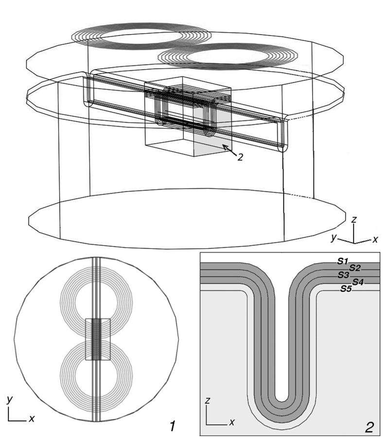
Overall geometry of the volume conductor and stimulation coil showing a rectangular box (ROI) centered under the coil; Inset 1) Volume conductor viewed from above; Inset 2) Geometry of the sulcus. There are 5 surfaces (S1-S5), parallel to each other and 1 mm apart, over which the stimulation mechanisms were evaluated. Surfaces S1 and S4 represent the boundaries of the cortex.

The decision to model a sharp conductivity transition at the GM-WM interface rather than a more gradual one simplifies considerably the construction of the computer model. However, it has been shown that, at least in the motor cortex, this interface is not well defined (Paxinos and Mai, 2004), with conductivity probably changing gradually from the cortex to the white matter. The actual jump of the electric field, ΔE_n, across the GM-WM interface in the motor cortex is probably smaller than the one assumed in our model. The issue of the scale of the interface is an important area requiring further study. Systematic FEM studies could be performed and should be addressed in forthcoming work.

The coil model is based on the Magstim Double 70 mm coil (P/N 9790), and is described in more detail in Thielscher and Kammer (2002, 2004) and in Miranda et al. (2007). The coil lies 1 cm above and parallel to the surface of the volume conductor, with its center just above the center of the sulcus, at (x, y, z)= (0, 0, 0.01) m. The axis of the coil is positioned perpendicularly to the axis of the sulcus and induces a posterior-anterior electric field in the cortex. The current in the coil is modeled as sinusoidal with a maximum rate of change of 67 A/μs, an average threshold value for monophasic P-A stimulation of the motor cortex with this coil (Kammer et al., 2001; Thielscher and Kammer, 2002). Thus, the peak electric field induced in the model should correspond approximately to the electric field induced in a real head at threshold. The temporal evolution of the electric field in the brain is determined solely by the time derivative of the current in the coil. However, this information is useful only if the membrane kinetics are built into the model, too. This aspect is not explored in this work.

The electric field induced by the coil in the brain tissues was calculated using the Finite Element Method (FEM) implemented by the commercial program Comsol Multiphysics (http://www.comsol.com). The total electric field, E⃗, induced in the brain tissues by TMS is given by

$$\overrightarrow{E}=-\frac{\partial \overrightarrow{A}}{\partial t}-\nabla \phi ,$$ (4)

where A⃗ is the magnetic vector potential and ∇φ is the gradient of the electric potential φ. The program calculates the spatial distribution of the two sources of the electric field, − ∂A⃗/∂t and −∇φ, as well as their sum. The global FEM mesh has 402,520 tetrahedral elements and 606,210 degrees of freedom. The average dimension of the finite elements inside the ROI is about 3 mm. Close to the sulcus and within it, the dimension of the elements is about 0.5 mm. The calculated values of the induced electric field near and within the cortical layer are expected to be accurate to within 10% or better. In an homogeneous medium with the assumed symmetry between coil and tissue interface, so there is no charge accumulation, the electric field is given solely by E⃗ = −∂A⃗/∂t. This part of the solution obtained in the heterogeneous model is the total electric field that would be induced in a homogeneous model.

Calculating the strength of the stimulation mechanisms along the direction of the axon

The magnitude of the three stimulation mechanisms was calculated for perpendicular and tangential orientations of the axons within the cortical sheet. At any point on the cortical surface, the perpendicular direction is uniquely defined by a unit vector normal to the surface, n⃗. In contrast, the tangent to the cortical surface only defines a plane. Assuming that the axons are isotropically distributed within the cortical layers, we report the maximum strength of a stimulation mechanism within the tangent plane, independent of its orientation within that plane.

The electric field term for perpendicular axons was therefore computed as − λ E_n = −λ (E⃗ · n⃗) = − λ E cos(θ), as shown in Fig. 2. A similar procedure was followed for the electric field term for the tangential axons, − λ E_t, additionally taking into account that the tangential electric field may have a component along the direction perpendicular to the plane of the figure. The calculation of the directional derivative of the electric field perpendicular to the cortical surface involves estimating the rate of change of the perpendicular component of the electric field, E_n, along the direction defined by n⃗. The procedure for doing this calculation is described elsewhere (Miranda et al., 2007). For the tangential directional derivative, the direction of the strongest gradient in the tangential plane was found first using the method of Lagrange multipliers and then the gradient along that tangential direction was calculated as above. Both the perpendicular and the tangential directional derivatives were multiplied by λ² to obtain estimates of the change in membrane potential. The electric field jump only affects the perpendicular component of the electric field and has magnitude of $-\lambda \frac{\Delta E_n}{2}$.

Fig. 2.

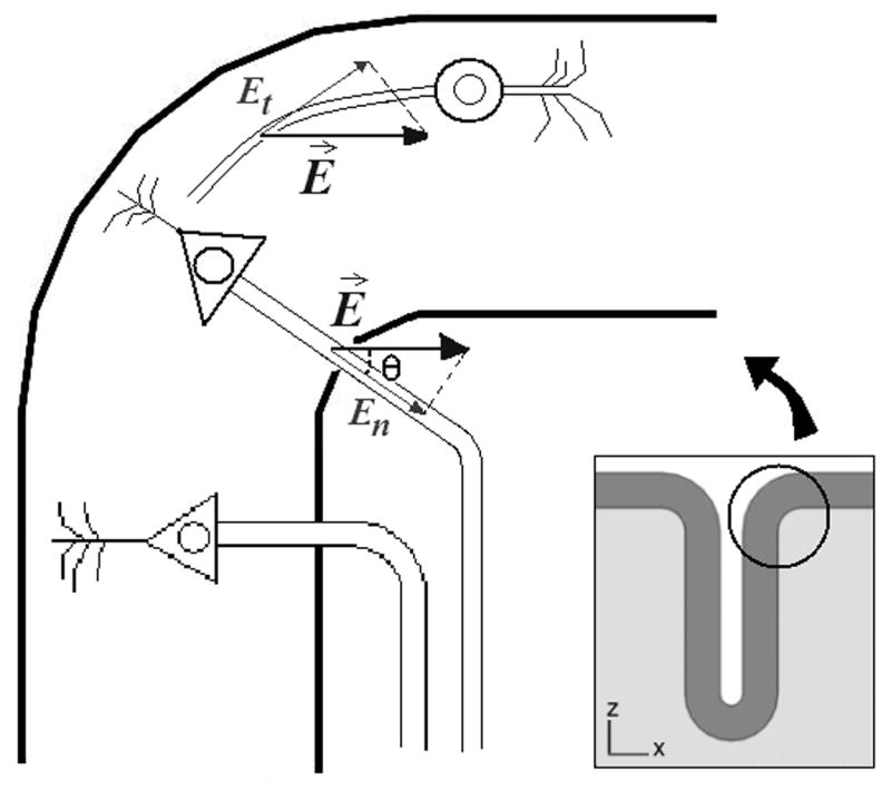
Projections of the electric field along the axon's axis, for different cells in the cortex. The projection of the electric field along a pyramidal axon is the component of E⃗ perpendicular to the cortical surface, E_n. The projection of the electric field along the axon of a horizontal cell is the component of E⃗ tangent to the cortical surface, E_t, since horizontal cells are oriented tangentially to the cortical surface.

We will refer to each of the stimulation mechanisms considered in this work as follows: the mechanisms related to the perpendicular and tangential components of E⃗ will be referred to by their mathematical expressions, − λE_n and − λ E_t, respectively; $-\lambda \frac{\Delta E_n}{2}$ will be referred to as the electric field jump mechanism; and the perpendicular and tangential directional derivatives multiplied by λ² will be referred to as the perpendicular directional derivative and the tangential directional derivative, respectively.

Data post-processing

The FEM simulations were performed using first order finite elements, and therefore only provided values for the two contributions to the total electric field: $-\frac{\partial \overrightarrow{A}}{\partial t}$, and −∇φ; however, calculating the directional derivatives of the electric field involves the calculation of the derivatives of all three components of the total electric field E⃗ = (E_x, E_y, E_z) with respect to all three coordinate directions (x, y, z) (Miranda et al., 2007). To do this, we exported the electric field data to Matlab (http://www.mathworks.com) in regular grids of 81×61×101 points, spanning the dimensions of the ROI. Appropriate functions were fitted along the lines and columns of the data matrices, respecting the electric field discontinuity at the interfaces. The two contributions to the total electric field were fitted separately, using a least-squares algorithm. Goodness-of-fit was assessed for each fit using the Wald-Wolfowitz runs test (Motulsky and Ransnas, 1987). An example of a fit to the z-component of the total electric field along a line of increasing depth (z-axis) is shown in Fig. 3. The electric field derivatives, ∂E_z / ∂z in the case of Fig. 3, were obtained by differentiating the fitted curve.

Fig. 3.

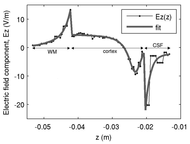
Fit of E_z along z. The data sets for each subdomain (CSF, cortex and WM) are fitted separately to calculate the electric field derivative, ∂E_z / ∂z, analytically.

Values for λ

Each stimulation mechanism targets different groups of cells, which have different space constants. The target cells of − λE_n and of the perpendicular directional derivative are corticospinal tract cells and corticocortical association fibers (both pyramidal cells), since they run perpendicular to the cortical surface, as well as perpendicularly aligned interneurons and pyramidal axon collaterals. The target cells of the electric field jump mechanism (evaluated over the GM-WM interface) are exclusively pyramidal. Targets for − λ E_t and the tangential directional derivative are expected to be interneurons' axons and collaterals of pyramidal axons that run tangential to the cortical surface.

Corticospinal tract fibers span a large range of external diameters, d₀, and can be divided into three categories according to their calibers: small fibers, 1-4 μm; medium fibers, 5-10 μm; and large fibers, 11-20 μm (Lassek, 1942). Using the scaling law for equivalent axons, λ = 117d₀, derived by Basser and Roth (1991) we can estimate the ranges of values of λ corresponding to the fiber categories established by Lassek (1942): 0.12-0.47 mm for small pyramidal fibers, 0.59-1.17 mm for medium fibers, and 1.29-2.34 mm for large (pyramidal) fibers.

Horizontal fibers and corticocortical association fibers in the human motor cortex are presumed to be smaller than the pyramidal tract fibers (Manola et al., 2007), although their diameters are largely unknown. We will take the intracortical fibers (either interneuronal axons or collaterals of pyramidal axons) as being small to medium caliber fibers. It should be noted that the smallest fibers in the pyramidal tract have diameters of about 1 μm (Lassek, 1942) while in the central nervous system myelinated fibers may exist with diameters as small as 0.2 μm (Waxman and Bennett, 1972; Ritchie, 1982). Predictions for the stimulation of horizontal fibers and intracortical perpendicular fibers should take into account this broader range of diameters.

As a first approximation, taking into consideration the ranges of values for λ and the fact that pyramidal cells are the most abundant nerve cells of the cerebral cortex, we will consider 1 mm to be a good estimate for the average value of λ. Also, since the fibers with the largest diameters are those with lower thresholds (Basser and Roth, 1991), we will also consider a maximum value of λ of 2 mm to represent large axons such as those of the Betz cells in the motor cortex.

Stimulation threshold

To establish a value for the stimulation threshold for a realistic TMS stimulus duration, we used the response V(t) of a homogenized passive cable equation for a myelinated axon as given in Basser and Roth (1991). The intrinsic threshold depolarization for neural stimulation is about 20 mV (Basser and Roth, 1991). For long stimuli, where the membrane potential reaches a new steady state, this is also the required strength for the stimulation mechanism since equations (1)-(3) assume a steady state. For short stimuli, the change in membrane potential will not reach the values specified by those equations, so higher stimulus intensity must be applied for effective stimulation. Using the transient response V (t) and taking a typical stimulus duration to be 150 μs (Barker at al., 1991), the threshold stimulus intensity must be such that the steady state depolarization would be about 52 mV. This is the value to which the various stimulation mechanisms (− λE_n, − λ E_t, the perpendicular directional derivative, the tangential directional derivative and the electric field jump mechanism) will be compared in order to establish whether stimulation would occur at a given location. If a stimulation mechanism reaches amplitudes higher than 52 mV, we assume that its targeted cells will be stimulated.

Results

Heterogeneous model versus homogeneous model

In order to assess the changes introduced by the heterogeneity of the volume conductor relative to an equivalent homogeneous model, the magnitude of the activation mechanisms was calculated in both the homogeneous and the heterogeneous models. The results are illustrated in Figs. 4, 5 and 6.

Fig. 4.

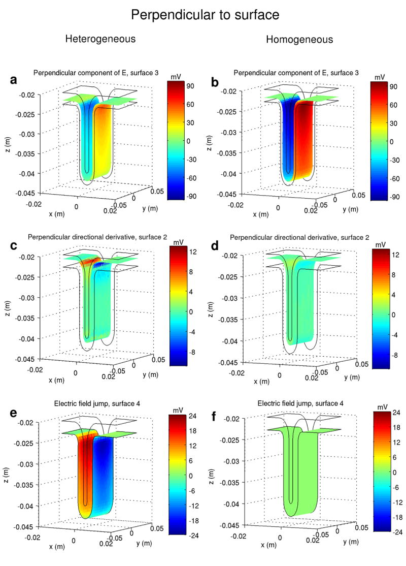
Comparison of the perpendicular projections of the different stimulation mechanisms in the heterogeneous model (left column) and in the equivalent homogeneous model (right column). “Perpendicular component of E” denotes − λE_n. Each stimulation mechanism is displayed over the same surface and for the same space constant (1 mm). For ease of comparison, the same scale is used for each horizontal pair of figures. The stimulation coil is positioned above and centered on the visualized volume (ROI, cf Fig. 1) and induces an electric field parallel to the P-A direction (+ x to − x).

Fig. 5.

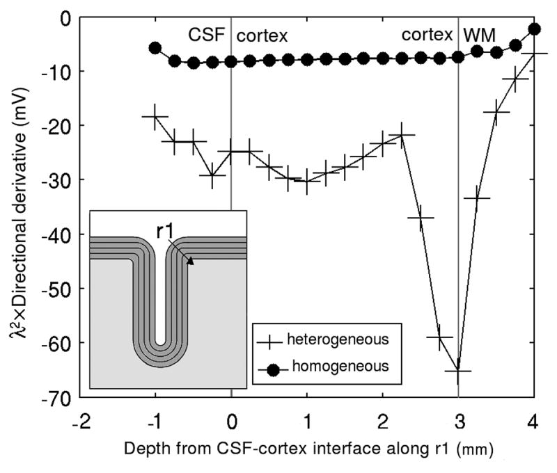
Effect of tissue heterogeneity on the gradient of the electric field: Comparison between the heterogeneous and the homogeneous models. The gradient is inspected along a line r1 perpendicular to the cortex (cf. inset) assuming a space constant of λ = 2 mm. The curved geometry of the cortex results in an increased gradient that may lead to stimulation of large pyramidal axons near the GM-WM interface.

Fig. 6.

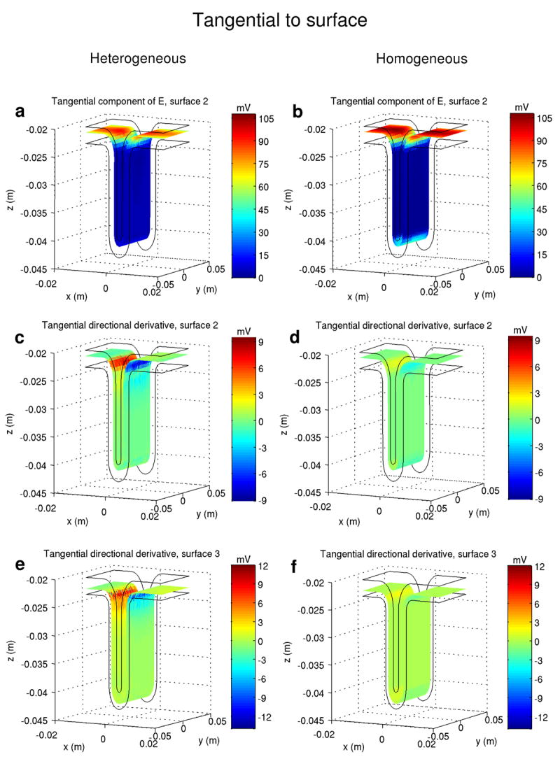
Comparison of the tangential projections of the stimulation mechanisms in the heterogeneous model (left column) and in the equivalent homogeneous model (right column). “Tangential component of E” denotes − λE_t. Each stimulation mechanism is displayed over the same surface and for the same space constant (1 mm). For ease of comparison, the same scale is used for each horizontal pair of graphics. The stimulation coil is positioned above and centered on the visualized volume (ROI, cf. Fig. 1) and induces an electric field parallel to the P-A direction (+ x to − x).

The amplitude of − λE_n in the heterogeneous model inside the cortex was about 30 to 40% less than the maximum value in the homogenous model (Figs 4.a and 4.b). This reduction is due to charge accumulation on the GM-WM interface. On the gray matter side, the term − ∇φ, which appears due to charge accumulation, opposes the term − ∂A⃗/ ∂t, resulting in a decrease of magnitude of the total electric field. On the white matter side of the interface, the total electric field is increased by the same amount. The amplitude of the perpendicular directional derivative (Figs. 4.c and 4.d) is higher in the heterogeneous model. For λ = 1 mm, the maximum value of this stimulation mechanism increases from 2 mV to about 13 mV, while for λ = 2 mm the maximum amplitude of this function increases from 8 mV to 52 mV. In Fig. 5 the amplitude of the perpendicular directional derivative in the two models is displayed along line r1, perpendicular to the cortex and passing through the point which defines the radius of curvature of the gyrus (cf. Fig. 5, inset). The curved geometry boosts this stimulation mechanism near the GM-WM interface, increasing its magnitude from about 10 mV to about 65 mV, for λ = 2 mm. As for the tangential mechanisms, the amplitude of − λ E_t (Figs. 6.a and 6.b) diminished by about 13% from the homogeneous model to the heterogeneous one. Finally, the maximum value of the tangential directional derivative (Figs. 6.c-6.f) increased about 5 times (from 2 mV to 9.5 mV) on the lip of the gyrus, from the homogeneous model to the heterogeneous one.

The mechanisms of stimulation in the heterogeneous model

Each stimulation mechanism should be evaluated in the relevant regions of the cortex, depending on the specific group of target cells. Therefore, − λE_n is evaluated on surface S5, tangential to the cortex and 1 mm below it (Fig. 1, inset 2), and inside the cortex, on surfaces S2 and S3, to inspect the stimulation of afferent axons, perpendicularly aligned interneuronal axons and collaterals of pyramidal axons. The perpendicular directional derivative is expected to stimulate the axons of pyramidal cells along their straight segments, perpendicular to the cortical surface. Below the GM-WM interface, the value of this function is small and will, therefore, be evaluated only inside the cortex and on the GM-WM interface (on surfaces S3 and S4, respectively). The electric field jump mechanism is evaluated on surface S4. Finally, − λ E_t and the tangential directional derivative should stimulate horizontal fibers and therefore both will be evaluated inside the cortex, on surfaces S2 and S3. We present the maximum values achieved by the stimulation mechanisms in the heterogeneous model, for λ = 1 mm.

The maximal amplitudes of − λE_n occur on the wall of the sulcus and also below the cortex, in the white matter, with a focal maximum under the coil center (y = 0) and just below the lip of the gyrus. On surface S3, this function reaches a value of 60 mV (Fig. 4.a), while on surface S5, in the white matter, it reaches a maximum value of 88 mV. On surface S5, where axons bend away from the electric field, the relevant figure is − λ E_n / 2 and reaches a maximum value of 44 mV. The mechanism of stimulation represented by − λ E_t achieves high amplitudes over the whole gyrus, covering the horizontal surfaces of the cortical model (Fig. 6.a). Its maximal values occur near the lip of the gyrus and below the coil center. On surface S2, − λ E_t reaches a value of 94 mV.

The remaining mechanisms of stimulation do not achieve sufficient amplitude for effective stimulation (52 mV): the maximum value achieved by the perpendicular directional derivative is 13.5 mV on the CSF-GM interface and 11 mV inside the cortex, on surface S3 (Fig. 4.c); the tangential directional derivative reached a value of 9.5 mV over surface S2 (Fig. 6.c) and the electric field jump mechanism achieved a maximum value of 25 mV, over surface S4, the GM-WM interface (Fig. 4.e).

The spatial patterns of these functions are independent of the value considered for λ. Their maximum values scale with λ for − λE_n, − λE_t and the electric field jump mechanism, and scale with λ² for the perpendicular and the tangential directional derivatives, respectively. These properties will be used in the Discussion to extend the comparison of the stimulation mechanisms to small, medium and large fibers.

Discussion

Effects of the heterogeneity of the volume conductor on the induced electric field

Our results show that, in the lip of the gyrus and along a line segment r1 perpendicular to the cortical surface (Fig. 5), the perpendicular directional derivative is much higher in the heterogeneous model that in the homogeneous model. In the heterogeneous model, and for λ = 2 mm, the perpendicular directional derivative in the lip of the gyrus may be responsible for the stimulation of pyramidal axons, while the magnitude of the same function in the homogeneous model is not sufficient to produce stimulation in the same conditions (Fig. 5). The magnitude and direction of the gradient of E⃗ depend on the geometry of the cortex, and are probably affected by the radius of curvature of the lip of the gyrus. In previous works (Kobayashi et al., 1997; Liu and Ueno, 2000) it was found that, during magnetic stimulation of peripheral nerves immersed in a heterogeneous medium, a longitudinal virtual cathode appears over the interface between two tissues. It was concluded that if a nerve fiber ran close and parallel to the interface, it could be stimulated by this virtual cathode; this source of stimulation was not present in a homogeneous model of the tissues surrounding the nerve fiber. Although, in these previous works, the conclusions were drawn for the stimulation of peripheral nerves with a tissue geometry quite different from the cortical geometry, the results obtained here are qualitatively similar, in terms of the effect of tissue heterogeneity on the outcome of magnetic stimulation.

The electric field jump mechanism cannot be assessed with a homogeneous model of the brain, since it arises from the differences in electrical conductivity between adjacent tissues. Yet, the results obtained in the heterogeneous model suggest that this stimulation mechanism may contribute to the activation of large diameter pyramidal neurons.

Globally, the heterogeneous model introduced an improvement in the estimates of the stimulation mechanisms with the lowest amplitudes, which tend to be underestimated (or even neglected) by the homogeneous models. These improvements seem to be relevant, since both stimulation mechanisms mentioned above (the perpendicular directional derivative and the electric field jump) may contribute to the loci of stimulation.

The mechanisms of stimulation in the heterogeneous model

By choosing a space constant of 1 mm, which corresponds to an axonal diameter d₀ of about 8.5 μm, we have addressed the stimulation of fibers in the medium caliber range. Then, the results presented above suggest that stimulation may occur due to − λE_n inside the cortex, in the region of the lip of the gyrus, for medium caliber (d₀ ≈ 8-10 μm) perpendicularly radiating intracortical fibers (if they exist in this range of diameters) and afferent axons terminating in the region of the maximum values of − λE_n. For this stimulation mechanism, V = 62 mV on S2 and V = 60 mV on S3. Stimulation may also occur due to − λ E_t, in the whole crown of the gyrus, for medium caliber horizontal fibers, if they exist in this range of diameters. For this mechanism, V = 94 mV on S2 and V = 92 mV on S3.

Predictions for the neuronal populations stimulated according to fiber diameter

For a realistic quantification of the stimulation mechanisms and of the actual loci of stimulation, a range of values for λ must be used, based on fiber size and type, as presented in the Methods section (see section “Values for λ”). Therefore, considering all the categories of nerve fibers and their corresponding ranges of values for λ, the results suggest that, under the TMS conditions modeled, stimulation of small fibers (d₀ < 4 μm), either pyramidal or other, is unlikely to occur. The largest value for the stimulation mechanisms obtained for this group of fibers (about 45 mV for − λ E_t and over surface S2) is below the estimated value for the stimulation threshold (52 mV). For pyramidal fibers of medium caliber (d₀: 5-10 μm), stimulation may occur outside the cortex, near the GM-WM interface in the wall of the sulcus, but only for the largest fibers in this group (d₀ = 10 μm). This is inferred from the results obtained over surface S5, where the maximum value of − λE_n / 2 varies between 26 mV and 52 mV for this group of fibers. For interneurons with medium caliber axons, if they exist, stimulation may occur in 1) horizontal fibers in the crown of the gyrus and aligned with the electric field (mainly y-axis, in the ROI), due to − λ E_t, for which the maximum values reached vary between 56 mV and 112 mV on S2 and between 53 mV and 107 mV on S3, and in 2) perpendicular fibers in the wall of the sulcus, due to − λE_n, for which the maximum value varies between 38 mV and 76 mV over surface S2. Finally, for large pyramidal fibers (d₀: 11-20 μm), stimulation may occur 1) outside the cortex where fibers bend sharply, due to − λE_n, for all axons in this range of diameters (where the maximum value of V varies between 63 and 103 mV on S5) and 2) inside the cortex and under the center of the coil, in the lip of the gyrus, due to the perpendicular directional derivative (V = 60 mV on S3) and on the GM-WM interface, due to the electric field jump mechanism (V = 59 mV), but only for the largest axons in this group of fibers (i.e., for the largest Betz cells).

To summarize, the results suggest that the loci of stimulation in our model of the cortex will be 1) terminations of medium caliber horizontal fibers located throughout the crown of the gyrus and aligned with the electric field, 2) terminations of medium caliber intracortical vertical axons, vertical pyramidal axon collaterals and terminations of pyramidal afferents, located in the lip of the gyrus and a few millimeters in depth from the lip of the gyrus, 3) bends of pyramidal fibers with d₀ ≥ 10 μm, in the white matter just below the lip of the gyrus, and 4) bends of Betz cells axons, in the vicinity of the whole surface of the vertical wall of the sulcus, with an expected maximum depth of stimulation of at least 1.5 cm below the cortical envelope.

At the motor threshold, − λE_n can only stimulate axons with diameters of at least 6.8 μm (i.e., for λ ≥ 0.8 mm), while − λ E_t can stimulate axons with diameters as small as 4.6 μm (i.e., for λ ≥ 0.54 mm). The remaining mechanisms can only activate fibers in the large diameter range. This may determine which nerve fibers will be stimulated first, whether interneurons, pyramidal cells or collaterals of pyramidal axons. Given the limited knowledge about the distribution of sizes of all the targeted cells in TMS, and in spite of the detail in the predictions presented here, the results are inconclusive concerning the D and I wave hypothesis. According to the results, TMS at threshold seems equally likely to stimulate medium caliber (d₀ ≥ 4.6 μm) interneurons in the gyri (I waves) and large pyramidal cells (d₀ ≥ 10 μm) in white matter near the wall of the sulcus (D waves). Nevertheless, the number of interneurons is much larger than the number of large pyramidal cells, and that may influence which type of response is more easily evoked by TMS. On the other hand, it is not known if interneurons of medium caliber exist in large numbers.

Concluding remarks

We used a simple heterogeneous and isotropic model of a cortical sulcus to investigate the effect of tissue heterogeneity on the spatial distribution of the induced electric field and some of its derived quantities. The results were used to make predictions about which neural populations are most likely to be stimulated by TMS, based on the maximum values obtained for each of the mechanisms of stimulations we considered. Greater detail in the geometry of the brain model, as well as inclusion of the tissues' anisotropic conductivity (Miranda et al., 2003; Holdefer et al., 2006; De Lucia et al., 2007) should provide better estimates of the TMS effects presented here. Another way to improve this cortical model is to embed neural trajectories in it to obtain the electric field along the neuron, and then use mathematical models of the neural response to the applied electric field to make predictions about stimulation sites in those neurons, without having to make assumptions about their geometry (e.g. long straight axons or sharp bends). Additionally, by modeling the membrane kinetics, it will be possible to predict the effect of stimulus waveform on the stimulation process. Continuing this line of research appears to be the only viable means of determining which of the several competing physical mechanisms of nerve excitation are at work in TMS of the cerebral cortex.

References

- Amassian VE, Eberle L, Maccabee PJ, Cracco RQ. Modelling magnetic coil excitation of human cerebral cortex with a peripheral nerve immersed in a brain-shaped volume conductor: the significance of fiber bending in excitation. Electroencephalogr Clin Neurophysiol. 1992;85:291–301. doi: 10.1016/0168-5597(92)90105-k. [DOI] [PubMed] [Google Scholar]
- Barker AT, Garnham CW, Freeston IL. Magnetic nerve stimulation: the effect of waveform on efficiency, determination of neural membrane time constants and the measurement of stimulator output. Electroencephalogr Clin Neurophysiol Suppl. 1991;43:227–237. [PubMed] [Google Scholar]
- Barker AT, Jalinous R, Freeston IL. Non-invasive magnetic stimulation of human motor cortex. Lancet. 1985;1:1106–1107. doi: 10.1016/s0140-6736(85)92413-4. [DOI] [PubMed] [Google Scholar]
- Basser PJ, Roth BJ. Stimulation of a myelinated nerve axon by electromagnetic induction. Med Biol Eng Comput. 1991;29:261–268. doi: 10.1007/BF02446708. [DOI] [PubMed] [Google Scholar]
- Baumann SB, Wozny DR, Kelly SK, Meno FM. The electrical conductivity of human cerebrospinal fluid at body temperature. IEEE Trans Biomed Eng. 1997;44:220–223. doi: 10.1109/10.554770. [DOI] [PubMed] [Google Scholar]
- Brodal P. The central nervous system: structure and function. 2nd. Oxford University Press Inc.; 1998. [Google Scholar]
- Day BL, Dressler D, Maertens de Noordhout A, Marsden CD, Nakashima K, Rothwell JC, Thompson PD. Electric and magnetic stimulation of human motor cortex: surface EMG and single motor unit responses. J Physiol. 1989;412:449–473. doi: 10.1113/jphysiol.1989.sp017626. [DOI] [PMC free article] [PubMed] [Google Scholar]
- De Lucia M, Parker GJM, Embleton K, Newton JM, Walsh V. Diffusion tensor MRI-based estimation of the influence of brain tissue anisotropy on the effects of transcranial magnetic stimulation. Neuroimage. 2007;36:1159–1170. doi: 10.1016/j.neuroimage.2007.03.062. [DOI] [PubMed] [Google Scholar]
- Di Lazzaro V, Oliviero A, Pilato F, Saturno E, Dileone M, Mazzone P, Insola A, Tonali PA, Rothwell JC. The physiological basis of transcranial motor cortex stimulation in conscious humans. Clin Neurophysiol. 2004;115:255–266. doi: 10.1016/j.clinph.2003.10.009. [DOI] [PubMed] [Google Scholar]
- Fox PT, Narayana S, Tandon N, Sandoval H, Fox SP, Kochunov P, Lancaster JL. Column-based model of electric field excitation of cerebral cortex. Hum Brain Mapp. 2004;22:1–14. doi: 10.1002/hbm.20006. [DOI] [PMC free article] [PubMed] [Google Scholar]
- Gabriel S, Lau RW, Gabriel C. The dielectric properties of biological tissues: II. Measurements in the frequency range 10 Hz to 20 GHz. Phys Med Biol. 1996;41:2251–2269. doi: 10.1088/0031-9155/41/11/002. [DOI] [PubMed] [Google Scholar]
- Gonçalves SI, de Munck JC, Verbunt JP, Bijma F, Heethaar RM, Lopes da Silva FH. In vivo measurement of the brain and skull resistivities using an EIT-based method and realistic models for the head. IEEE Trans Biomed Eng. 2003;50:754–767. doi: 10.1109/tbme.2003.812164. [DOI] [PubMed] [Google Scholar]
- Hallett M. Transcranial magnetic stimulation and the human brain. Nature. 2000;406:147–150. doi: 10.1038/35018000. [DOI] [PubMed] [Google Scholar]
- Haueisen J, Ramon C, Eiselt M, Brauer H, Nowak H. Influence of tissue resistivities on neuromagnetic fields and electric potentials studied with a finite element model of the head. IEEE Trans Biomed Eng. 1997;44:727–735. doi: 10.1109/10.605429. [DOI] [PubMed] [Google Scholar]
- Holdefer RN, Sadleir R, Russell MJ. Predicted current densities in the brain during transcranial electrical stimulation. Clin Neurophysiol. 2006;117:1388–1397. doi: 10.1016/j.clinph.2006.02.020. [DOI] [PMC free article] [PubMed] [Google Scholar]
- Kammer T, Beck S, Thielscher A, Laubis-Herrmann U, Topka H. Motor thresholds in humans: a transcranial magnetic stimulation study comparing different pulse waveforms, current directions and stimulator types. Clin Neurophysiol. 2001;112:250–258. doi: 10.1016/s1388-2457(00)00513-7. [DOI] [PubMed] [Google Scholar]
- Knecht S, Sommer J, Deppe M, Steinstrater O. Scalp position and efficacy of transcranial magnetic stimulation. Clin Neurophysiol. 2005;116:1988–1993. doi: 10.1016/j.clinph.2005.04.016. [DOI] [PubMed] [Google Scholar]
- Kobayashi M, Ueno S, Kurokawa T. Importance of soft tissue inhomogeneity in magnetic peripheral nerve stimulation. Electroencephalogr Clin Neurophysiol. 1997;105:406–413. doi: 10.1016/s0924-980x(97)00035-0. [DOI] [PubMed] [Google Scholar]
- Kozel FA, Nahas Z, deBrux C, Molloy M, Lorberbaum JP, Bohning D, Risch SC, George MS. How coil-cortex distance relates to age, motor threshold, and antidepressant response to repetitive transcranial magnetic stimulation. J Neuropsychiatry Clin Neurosci. 2000;12:376–384. doi: 10.1176/jnp.12.3.376. [DOI] [PubMed] [Google Scholar]
- Lassek AM. The human pyramidal tract. IV. A study of the mature, myelinated fibers of the pyramid. J Comp Neurol. 1942;76:217–225. [Google Scholar]
- Liu R, Ueno S. Calculating the activating function of nerve excitation in inhomogeneous volume conductor during magnetic stimulation using the finite element method. IEEE Trans Magn. 2000;36:1796–1799. [Google Scholar]
- Maccabee PJ, Amassian VE, Eberle LP, Rudell AP, Cracco RQ, Lai KS, Somasundarum M. Measurement of the electric field induced into inhomogeneous volume conductors by magnetic coils: application to human spinal neurogeometry. Electroencephalogr Clin Neurophysiol. 1991;81:224–237. doi: 10.1016/0168-5597(91)90076-a. [DOI] [PubMed] [Google Scholar]
- Manola L, Holsheimer J, Veltink P, Buitenweg JR. Anodal vs cathodal stimulation of motor cortex: A modeling study. Clin Neurophysiol. 2007;118:464–474. doi: 10.1016/j.clinph.2006.09.012. [DOI] [PubMed] [Google Scholar]
- Mills KR, Boniface SJ, Schubert M. Magnetic brain stimulation with a double coil: the importance of coil orientation. Electroencephalogr Clin Neurophysiol. 1992;85:17–21. doi: 10.1016/0168-5597(92)90096-t. [DOI] [PubMed] [Google Scholar]
- Miranda PC, Correia L, Salvador R, Basser PJ. Tissue heterogeneity as a mechanism for localized neural stimulation by applied electric fields. Phys Med Biol. 2007;52:5603–5617. doi: 10.1088/0031-9155/52/18/009. [DOI] [PubMed] [Google Scholar]
- Miranda PC, Hallett M, Basser PJ. The electric field induced in the brain by magnetic stimulation: a 3-D finite-element analysis of the effect of tissue heterogeneity and anisotropy. IEEE Trans Biomed Eng. 2003;50:1074–1085. doi: 10.1109/TBME.2003.816079. [DOI] [PubMed] [Google Scholar]
- Motulsky HJ, Ransnas LA. Fitting curves to data using nonlinear regression: a practical and nonmathematical review. FASEB J. 1987;1:365–374. [PubMed] [Google Scholar]
- Mountcastle VB. The columnar organization of the neocortex. Brain. 1997;120:701–722. doi: 10.1093/brain/120.4.701. [DOI] [PubMed] [Google Scholar]
- Nagarajan SS, Durand DM, Warman EN. Effects of induced electric fields on finite neuronal structures: a simulation study. IEEE Trans Biomed Eng. 1993;40:1175–1188. doi: 10.1109/10.245636. [DOI] [PubMed] [Google Scholar]
- Nolte J. The human brain: an introduction to its functional anatomy. 5th. Mosby; 2002. [Google Scholar]
- Paxinos G, Mai JK. The human nervous system. 2nd. Elsevier; Academic Press; 2004. p. 1013. [Google Scholar]
- Ritchie JM. On the relation between fibre diameter and conduction velocity in myelinated nerve fibres. Proc R Soc Lond B Biol Sci. 1982;217:29–35. doi: 10.1098/rspb.1982.0092. [DOI] [PubMed] [Google Scholar]
- Robillard PN, Poussart Y. Specific-impedance measurements of brain tissues. Med Biol Eng Comput. 1977;15:438–445. doi: 10.1007/BF02457999. [DOI] [PubMed] [Google Scholar]
- Roth BJ. Mechanisms for electrical stimulation of excitable tissue. Crit Rev Biomed Eng. 1994;22:253–305. [PubMed] [Google Scholar]
- Roth BJ, Basser PJ. A model of the stimulation of a nerve fiber by electromagnetic induction. IEEE Trans Biomed Eng. 1990;37:588–597. doi: 10.1109/10.55662. [DOI] [PubMed] [Google Scholar]
- Rushton WAH. A theory of the effects of fibre size in medullated nerve. J Physiol. 1951;115:101–122. doi: 10.1113/jphysiol.1951.sp004655. [DOI] [PMC free article] [PubMed] [Google Scholar]
- Rushton WAH. The effect upon the threshold for nervous excitation of the length of nerve exposed, and the angle between current and nerve. J Physiol. 1927;63:357–377. doi: 10.1113/jphysiol.1927.sp002409. [DOI] [PMC free article] [PubMed] [Google Scholar]
- Standring S. Gray's anatomy: The anatomical basis of clinical practice. 39th. Elsevier Churchill Livingstone; 2005. [Google Scholar]
- Stokes MG, Chambers CD, Gould IC, Henderson TR, Janko NE, Allen NB, Mattingley JB. Simple metric for scaling motor threshold based on scalp-cortex distance: application to studies using transcranial magnetic stimulation. J Neurophysiol. 2005;94:4520–4527. doi: 10.1152/jn.00067.2005. [DOI] [PubMed] [Google Scholar]
- Terao Y, Ugawa Y. Basic mechanisms of TMS. J Clin Neurophysiol. 2002;19:322–343. doi: 10.1097/00004691-200208000-00006. [DOI] [PubMed] [Google Scholar]
- Thielscher A, Kammer T. Electric field properties of two commercial figure-8 coils in TMS: calculation of focality and efficiency. Clin Neurophysiol. 2004;115:1697–1708. doi: 10.1016/j.clinph.2004.02.019. [DOI] [PubMed] [Google Scholar]
- Thielscher A, Kammer T. Linking physics with physiology in TMS: a sphere field model to determine the cortical stimulation site in TMS. Neuroimage. 2002;17:1117–1130. doi: 10.1006/nimg.2002.1282. [DOI] [PubMed] [Google Scholar]
- Waxman SG, Bennett MV. Relative conduction velocities of small myelinated and non-myelinated fibres in the central nervous system. Nat New Biol. 1972;238:217–219. doi: 10.1038/newbio238217a0. [DOI] [PubMed] [Google Scholar]
- Yousry TA, Schmid UD, Alkadhi H, Schmidt D, Peraud A, Buettner A, Winkler P. Localization of the motor hand area to a knob on the precentral gyrus - A new landmark. Brain. 1997;120:141–157. doi: 10.1093/brain/120.1.141. [DOI] [PubMed] [Google Scholar]