How Long Will My Mouse Live? Machine Learning Approaches for Prediction of Mouse Life Span

Abstract

Prediction of individual life span based on characteristics evaluated at middle-age represents a challenging objective for aging research. In this study, we used machine learning algorithms to construct models that predict life span in a stock of genetically heterogeneous mice. Life-span prediction accuracy of 22 algorithms was evaluated using a cross-validation approach, in which models were trained and tested with distinct subsets of data. Using a combination of body weight and T-cell subset measures evaluated before 2 years of age, we show that the life-span quartile to which an individual mouse belongs can be predicted with an accuracy of 35.3% (±0.10%). This result provides a new benchmark for the development of life-span–predictive models, but improvement can be expected through identification of new predictor variables and development of computational approaches. Future work in this direction can provide tools for aging research and will shed light on associations between phenotypic traits and longevity.

PREDICTION of individual life span represents a significant challenge for aging research that is important for understanding factors influencing longevity, as well as identifying life-span–associated characteristics that can be studied as surrogates of longevity in laboratory experiments. In mice, previous studies have identified early- and mid-life traits that correlate with life span and have developed models for life-span prediction (1–11). These investigations have provided insight into links between phenotypic characteristics and mechanisms that regulate longevity. Low body weight, for example, has been associated with increased life span in genetically heterogeneous mouse populations (8,11). This association may reflect population-level variability in growth hormone/insulin-like growth factor-1 (GH/IGF-1) signaling, because mutations inhibiting this pathway have been found to increase life span while decreasing body weight in mice (12). Models that predict life span also offer the possibility of accelerating aging research. Full-length survivorship studies require several decades to complete in monkeys (13,14), and require at least 3 years to complete using healthy mouse strains (15). Forecasting of individual life span based on noninvasive predictors would provide preliminary data years in advance. The prediction of individual longevity, however, represents a daunting task, and is complicated by numerous sources of genetic and environmental variability (16–18). Nevertheless, the potential value of models that accurately predict life span is considerable, and efforts directed toward formulating such models will advance our understanding of factors regulating longevity.

There are two complementary areas of research from which progress in life-span prediction can be anticipated. The first of these involves generation of data sets including a range of predictor variables as well as outcomes of interest, such as life span, disease risk, and indices of age-dependent functional decline against which candidate predictors can be evaluated. The second element focuses on determining which statistical methods are best able to integrate results from a panel of predictors into a single model. A predictive model represents a pattern connecting a set of quantitative characteristics to individual life span. Such patterns, however, may be highly complex and difficult to characterize in simple mathematical terms, for example, in the form of a regression equation. If presented with a series of facial photographs, for example, we can quickly discriminate young from middle-aged adults with excellent accuracy. This task, however, requires a highly sophisticated pattern-recognition device (the human brain), and it is very difficult to write a mathematical model that relates the visual image to the age of the person depicted. Sophisticated modeling approaches may therefore be necessary to characterize patterns that connect predictor variables to longevity and other age-sensitive end points of interest. Previous studies have characterized relationships between predictor variables and life span using least-squares regression (5–9,11). The advantage of this approach is the strong statistical foundation of least-squares regression procedures, which allows for robust statistical inferences when parametric assumptions are satisfied. A disadvantage, however, is that complex and nonlinear relationships may not be adequately captured by regression models. Large data sets, in particular, are valuable for exploring patterns between different traits and life span, but are not well suited to standard regression approaches. The statistical power associated with large data sets may impart statistical significance to small effect sizes of little biological importance. The validity of this statistical inference, moreover, tends to break down in large data sets, because multicollinearity among predictor variables accumulates as more variables are incorporated into models (19).

Machine learning algorithms are valuable tools for the generation of predictive models and identification of complex patterns between variables. These methods are used to predict an outcome of interest based on a set of predictor variables, and are especially well suited to large data sets for which least-squares regression approaches can be problematic. The approach is to present algorithms with a set of training cases, each of which consists of measurements on a set of predictor variables and a class label. For example, training cases may consist of mice measured for body weight, tail length, and body fat percentage (predictor variables), and each mouse is labeled as “short-lived” or “long-lived.” Within this framework, predictive models are generated as the algorithm “learns” a relationship between predictor variables and class labels. The manner by which learning occurs varies among algorithms, but may involve building a decision tree structure, identifying appropriate weights in a neural network, or identifying a maximal margin hyperplane that distinguishes training examples of different classes (20). These approaches have most often been applied in the context of handwritten digit recognition, speech pattern identification, and recognition of facial images (21,22). In recent years, however, machine learning has made important contributions to the biological sciences as well, and has been used to annotate gene sequence data (23), diagnose disease (24), and identify compounds with drug activity (25,26). Currently available methods range from classical approaches, such as linear and quadratic discriminant function classifiers, to more recently developed methods, which include decision trees, neural networks, and support vector machines (SVMs).

In this article, we use machine learning to predict mouse life span based on characteristics evaluated prior to 2 years of age. The data set we evaluate includes more than 1000 mice in which a wide range of characteristics have been measured, including T-cell subsets, serum hormone levels (IGF-1, leptin, and thyroxine), body weight, and cataract scores. Previous studies have found these variables to correlate with mouse life span using regression-based approaches (5–9,11), and have identified multivariate patterns related to life span (6). In this report, we evaluate the predictive capacity of variables using machine learning and a stringent evaluation criterion based on cross-validation. In this approach, machine learning models are constructed and evaluated using nonoverlapping sets of observations (drawn at random from the same mouse population). We can in this way evaluate how accurately mouse life span is predicted when models are applied to new animals not used in model construction. This approach provides an assessment of model “generalization ability,” which is of great importance for determining the usefulness of models in practical contexts (20). The framework we present provides a new perspective on the use of phenotypic characters as prognostic tools in aging research, and our results represent a novel benchmark for future work aimed at prediction of life span.

Methods

Experimental Animals

Data were collected from a genetically heterogeneous stock of mice generated by crossing (BALB/cJ × C57BL6/J)F1 (CB6F1) females with (C3H/HeJ × DBA/2J)F1 (C3D2F1) males. Mice derived from this cross are genetically unique, but share 50% of genes with other members of the population. The genetic composition of this stock thus minimizes the chance that findings will apply only to a single inbred or F1 hybrid genotype (15,27). Standard maintenance protocols used for this stock have been described previously (7,11). In brief, mice were weaned at 19–21 days of age and maintained in cages containing 3–4 mice of the same sex. Nonvirgin (“mated”) female mice were produced by introducing a male mouse into cages containing 3–4 female mice when the females were 2 months old. Litters were then removed from these cages within the first week after birth, and the male was removed when the females were 6 months old. Throughout the study, free access to laboratory chow and fresh water was provided, and sentinel animals were exposed to spent bedding on a quarterly basis to check for possible pathogen infection. Three animals were killed following detection of mouse Parvovirus, but no evidence of pinworm, Sendai virus, mycoplasma, or coronavirus was obtained during the study period. All cages were inspected on a daily basis to evaluate the health of the animals and to check for mortalities. Mice found to be extremely ill were killed, and the date of death was recorded as the most likely date of natural death.

Life Span Predictor Variables

Table 1 describes measurements obtained during the study that serve as potential life-span predictors in the present analysis. Variables include T-cell subset scores evaluated at 8 and 18 months of age, serum hormone levels at 4 and 15 months of age, body weight at 8–18 months of age, and cataract scores at 18 and 24 months of age. Several predictor variables listed in Table 1 have previously been identified as significantly correlated with mouse life span. Miller (6) showed that, within individual gender categories, variables CD4_8, CD8M_8, CD4V_8, CD4_18, CD4M_18, CD8M_18, CD4V_18, and CD4P_18 were significantly correlated with life span. A later investigation revealed that combining these variables using principal component analysis provided an index with an even stronger association with longevity (7). Miller and colleagues (8) focused on body weight measurements, and found that body weight between the ages of 2 and 24 months was correlated with life span, such that smaller mice were long-lived as compared to larger mice. Harper and colleagues (9) investigated hormone levels as potential predictors of life span, and reported that LEP_4, T4_4, and IGF_15 were correlated with both body weight and life span. Surprisingly, Harper and colleagues (9) also found significantly greater longevity among mice with more advanced cataract formation (higher Cat24 scores). Harper and colleagues (11) confirmed, in a replicate cohort, that CD8M_8, CD8M_8, and CD4_18 were significantly correlated with longevity, and also found that CD8_18 and CD8P_18 were associated with life span. In addition, Harper and colleagues (11) reported that the combination of T-cell subset and body weight measures significantly increased the variation in life span that was explained by regression models, compared to models based only on T-cell or weight predictors individually.

Table 1.

Predictor Variables.

Variable ID	Age (Months)	Description
T-cell subsets
CD3_8	8	Total T-cell marker, as a proportion of peripheral blood lymphocytes
CD3_18	18	As above
CD4_8	8	CD3+, CD4+, helper T cells, as a proportion of CD3 cells
CD4_18	18	As above
CD4M_8	8	CD4+, CD44high memory CD4 cells, as a proportion of CD4 cells
CD4M_18	18	As above
CD4P_8	8	CD4+ cells expressing P-glycoprotein, as a proportion of CD4 cells
CD4P_18	18	As above
CD4V_8	8	CD4+, CD45RBlow naive CD4 cells, as a proportion of CD4 cells
CD4V_18	18	As above
CD8_8	8	CD3+, CD8+, killer T cells, as a proportion of CD3 cells
CD8_18	18	As above
CD8M_8	8	CD8+, CD44high memory CD8 cells, as a proportion of CD8 cells
CD8M_18	18	As above
CD8P_8	8	CD8+ cells expressing P-glycoprotein, as a proportion of CD8 cells
CD8P_18	18	As above
Hormones
T4_4	4	Serum thyroxine (μg/dL)
T4_15	15	As above
LEP_4	4	Serum leptin (ng/mL)
LEP_15	15	As above
IGF_4	4	Serum IGF-I (ng/mL)
IGF_15	15	As above
Body weight
W8	8	Body weight
W10	10	As above
W12	12	As above
W18	18	As above
Other
LitSize	N/A	No. of pups in litter
Cat18	18	Cataract score, corrected for secular trend
Cat24	24	As above
Gender1	N/A	Indicator variable defined as 1 if sex = male, 0 otherwise
Gender2	N/A	Indicator variable defined as 1 if sex = female, 0 otherwise

Note: Table lists the age at which data were obtained and provides a brief description of each variable. See (5–9) and (11) for further description of variables.

Data Preprocessing

The complete data set includes age at death and predictor variable measurements for 1188 mice (403 virgin males, 457 virgin females, 299 mated females). The data are pooled from two survivorship studies that have been referred to as LAG1 and LAG2 in previous publications (11). We eliminated 183 cases in which mice had died prematurely from mouse urinary syndrome or had been removed from colonies because of fighting. Additionally, mice dying within the first 2 years of life were not considered in the analysis. This was done because all predictor variables were recorded within the first 2 years of life, and it was of interest to predict the longevity of mice surviving beyond this 2-year time frame. After this preprocessing, the data set contained 741 mice, all of which died of apparently natural causes beyond 2 years of age.

The 741 mice were each assigned to a life-span quartile based on age at death, and life-span quartile was used as the primary response variable in all analyses. This was done because many machine learning algorithms have been designed to predict categorical, rather than continuous, outcomes. Focusing on life-span quartiles therefore allowed us to implement a wider range of machine learning techniques. In addition, predicting categorical outcomes allows success to be measured in terms of an accuracy or error rate, which is useful for judging the performance of algorithms, as well as the quality of predictor variable subsets (20). For virgin males, life-span quartiles were assigned based on a 25th percentile life span of 811 days, a 50th percentile of 890 days, and a 75th percentile of 1034 days. Among virgin females, corresponding 25–50–75 percentile life spans were 811, 892, and 978 days, respectively. For mated females, these values were 790, 855, and 954 days, respectively.

All continuous variables were standardized to have a mean of zero and variance of one, and in some cases were log-transformed to attenuate the influence of outliers. Because a complete set of predictor variable measurements was not available for all mice, it was necessary to impute for missing data. For the discontinuous variable “LitSize,” we calculated the most commonly occurring value among all mice, and substituted this value in place of missing data. All other variables with missing data were continuous. In these cases, we calculated the median value among all observations, added a small amount of random noise, and substituted the obtained value for missing data. Substitution with median values is one of several possible approaches for dealing with missing data (28). The rationale is that variable values further away from the median are more influential in generating predictive models, such that substitution of the median value is neither helpful nor unhelpful for life-prediction.

Machine Learning and Life-Span Prediction

Machine learning methods vary considerably in their complexity, and it is uncertain for any particular application which algorithm will provide the best overall performance (20). The best algorithm depends on the quality of predictor variables and the “decision boundaries” that best distinguish mice belonging to different life-span quartiles (Figure 1). If quartiles are clearly separated by linear decision boundaries, simple algorithms may predict life-span quartile with high accuracy (see Figure 1A). In contrast, if quartiles can only be separated by complex, irregular decision boundaries, accurate prediction of life-span quartile will require more sophisticated algorithms (see Figure 1B). We therefore applied many algorithms to determine which approaches provide the best results for prediction of life-span quartile (Table 2). The manner by which algorithms generated predictions varied considerably among the different methods. Some algorithms generated predictions by constructing regression models (simple linear regression, multinomial logistic regression), whereas others constructed decision trees or sets of classification rules (e.g., binary decision trees, random forest, Ripper rule learner). Other algorithms fit probability models to mice associated with each life-span quartile, and used posterior class probability as a basis for prediction (e.g., naive Bayes). In some cases, predictions were generated in nonparametric fashion without construction of a formal classification model (e.g., k-nearest neighbor, nearest centroid, nearest shrunken centroid [NSC]). All algorithms were implemented using the R statistical software package. Specific functions of the R extension package used to implement each algorithm are listed in Table 2, and full descriptions of each package and function can be accessed online (http://www.r-project.org/).

Figure 1.

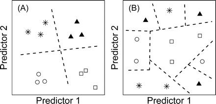
Simple and complex relationships between predictor variables and life span. Each plot displays data for 12 individuals in relation to scores on two predictors. The four symbol types represent individuals associated with each life-span quartile. A, Simple relationship between predictors and life span. Individuals associated with different life-span quartiles are distinguished by simple linear decision boundaries (dotted lines). Simple learning algorithms may perform well in comparison to complex algorithms. B, Complex relationship between predictors and life span. Individuals associated with different life-span quartiles can only be distinguished through recognition of irregular decision regions. Complex learning algorithms are required for accurate prediction of life span based on the two predictors

Table 2.

Algorithm Performance Summary.

Method	31 Predictors	12 Predictors	6 Predictors
Nearest Shrunken Centroid*	32.86	33.61	34.37
Stabilized Linear Discriminant Analysis†	30.50	34.06	32.30
Support Vector Machine‡	29.90	34.03	33.57
Gaussian Process§	30.29	32.81	33.90
Conditional Inference Tree Forest‖	29.88	33.49	32.65
Random Forest¶	30.18	33.34	29.36
Support Vector Machine**	29.56	33.27	31.54
Nearest Centroid††	30.86	33.16	32.43
Localized Linear Discriminant Analysis‡‡	27.29	32.44	32.06
Naive Bayes§§	29.14	32.19	31.16
Projection Pursuit Linear Discriminant Analysis Tree ‖ ‖	28.45	31.93	31.28
Linear Discriminant Analysis¶¶	27.03	31.86	31.16
Multinomial Logistic Regression***	27.02	31.78	31.14
Stump Decision Trees†††	30.46	30.50	31.15
Artificial Neural Network‡‡‡	27.94	30.50	30.90
Binary Decision Trees§§§	30.06	30.18	30.87
Conditional Inference Tree ‖ ‖ ‖	30.03	29.60	30.55
K-Nearest Neighbor¶¶¶	26.75	29.11	28.31
C4.5 Decision Tree****	27.43	28.03	29.07
Part Decision Tree††††	27.16	28.99	28.60
Simple Linear Regression‡‡‡‡	27.04	28.79	27.04
Ripper Rule Learner§§§§	25.82	26.10	25.43
Random Guessing‖ ‖ ‖ ‖	24.99	25.02	25.01

Notes: Life-span quartile prediction accuracy was evaluated for 22 machine learning algorithms using all 31 predictor variables, the 12 most important predictors, and the 6 most important predictors. Variable importance was determined based on the Random Forest algorithm (see Figure 4). Algorithms are ranked according their best overall performance among the three predictor variable subsets. For each listed value, accuracy is based on 10,000 simulations in which 664 mice (90%) were randomly selected as training data and used in model construction, with 77 mice (10%) used as testing data for model evaluation (see Methods). For each simulation, the average number of correct life-span quartile predictions among 77 testing set mice was determined. Table lists the average percent accuracy obtained among all 10,000 simulations (95% confidence intervals are approximately ± 0.10%). The R package and function used to implement each algorithm is given in brackets [package, function].

*Algorithm of Tibshirani and colleagues (29). Similar to Nearest Centroid approach, except class centroids are standardized and “shrunk” toward an overall centroid before evaluation of test cases. [pamr, pamr.train]

^†Left-spherically distributed linear scores are derived from predictor variables following the dimensionality reduction rule of Laeuter and colleagues (30). Linear scores are used as inputs for standard linear discriminant analysis. [ipred, slda]

^‡Predictor variables are mapped to a higher dimensional space using a specified kernel function. A linear hyperplane is identified with the largest possible margin between the two classes to be distinguished, and this “maximal margin” hyperplane is used to classify test cases. The listed accuracies were obtained using a polynomial kernel function, with model parameters chosen by searching possible values and identifying those that minimize prediction errors on the training data. An introduction to support vector machines is provided by Byvatov and Schneider (31). [e1071, svm]

^§Training data are modeled as a Gaussian Process, with mean and covariance functions partly determined by parameters estimated during model training. Within this framework, class probabilities associated with each test case are estimated, as described by Williams and Barber (32). Density estimation was performed using the radial basis kernel. [kernlab, gausspr]

^‖Similar to Random Forest, except conditional inference trees are used as a base classifier. Listed accuracy obtained using 100 decision trees per forest. [party, cforest]

^¶Algorithm of Breiman (33). Predictor variables and training examples are randomly selected to construct a “forest” of decision trees. Test cases are then classified by a voting procedure among all trees in the forest. Listed accuracy was obtained by growing 1000 decision trees per simulation. [randomForest, randomForest]

**Implements support vector training method of Platt (34). [RWeka, SMO]

^††Centroids are computed for each class using the training data. Test cases are then assigned the class label of the most similar centroid. [klaR, nm]

^‡‡Implements the linear discriminant analysis approach proposed by Tutz and Binder (35). [klaR, loclda]

^§§A probability density function is estimated for each class based on training data. For each test case, the estimated density is used to compute the probability of class membership for each class (assuming conditional independence of class-conditional probabilities). Test cases are assigned to the class for which its class-conditional probability is greatest. [klaR, NaiveBayes]

^{‖ ‖}Decision tree in which projection pursuit linear discriminant functions are used as attributes at each node (36). [classPP, PP.tree]

^¶¶Linear combinations of predictor variables are constructed to maximize the ratio of variation between classes versus the variance within classes. This provides a subspace of predictors with lower dimensionality that is used for classification of test cases. [klaR, lda]

***Multinomial logistic regression models based on ridge regression. See le Cessie and van Houwelingen (37). [RWeka, Logistic]

^†††Binary decision trees are constructed using only one predictor variable. [Rweka, DecsionStump]

^‡‡‡A neural network with one hidden layer and four output nodes (one for each class); the number of input nodes equals the number of predictor variables. During the training stage, a set of network weights that minimizes training errors is iteratively identified, and determines the contribution of each input variable to the overall network response. Basheer and Hajmeer (38) provide an introduction to this approach. [nnet, nnet]

^§§§Binary decision trees grown by recursive partitioning. Predictor variables were split to maximize information gain. [tree, tree]

^{‖ ‖ ‖}Two-step algorithm of Hothorn and colleagues (39). The variable most strongly associated with class labels among training examples is selected, and a decision tree branch is formed through a binary split of this chosen variable. The process repeats until all predictors significantly associated with class labels (at level α) have been incorporated. Listed accuracy obtained using α = 0.30. [party, ctree]

^¶¶¶For each test case, the k most similar observations among the training data are identified. The test case is assigned the most frequently occurring class label among the k most similar training observations. Listed accuracy obtained for k = 5. (see 40). [klaR, knn]

****Decision tree induction following Hunt's algorithm, in which trees are recursively grown by splitting attributes to maximize information gain (41). [RWeka, J48]

^††††Partial decision trees (42). [RWeka, PART]

^‡‡‡‡Least-squares multiple regression. Life-span quartile is treated as a numeric ordinal variable, and model selection is performed using the Akaike Information Criterion. [RWeka, LinearRegression]

^§§§§Test cases are classified according to a series of “if…then” rules extracted from training data using the RIPPER algorithm (43). [RWeka, JRip]

^{‖ ‖ ‖ ‖}No model building is performed, and class labels are randomly assigned to test cases.

If predictive models are trained and evaluated using the same data, it is always possible to generate a model that predicts with 100% accuracy. This can be done, for example, by constructing an overfit regression model with a large number of parameters. The predictive performance of such a model, however, would be sensitive to chance variation or noise in the training samples chosen to construct the model. Consequently, the model would lack “generalization ability” and would not be useful as a prognostic tool (20). The ability of an algorithm to produce generalizable results can be tested by using cross-validation to evaluate prediction accuracy, a process in which the model is trained by using one set of data, and its prediction accuracy evaluated by using a another, distinct set of data. This evaluation procedure is commonly used in the development of predictive models, and is necessary for providing a realistic assessment of how useful a model can be in practical scenarios in which the interest is to forecast results based on predictor variables from new observations (e.g., partially complete survivorship studies). Our analysis therefore used cross-validation to evaluate the accuracy of each algorithm for prediction of life-span quartile. Approximately 90% of the 741 mice were randomly selected as “training data,” with the remaining 10% of mice serving as “testing data.” Machine learning models were constructed using only the training data, and the resulting model was then applied to the testing data to determine prediction accuracy. The process of randomly parsing observations into training and testing sets, training the algorithm, and applying the algorithm to test data was repeated 10,000 times for each algorithm evaluated. Training data sets were always constructed such that an equal number of cases from each life-span quartile were presented to the algorithm. Testing data sets contained approximately 20 cases from each life-span quartile. The average prediction accuracy attained by each algorithm was compared to that expected from random guessing (25%). A 95% confidence interval (CI) was calculated for each average prediction accuracy and was used to evaluate whether accuracy was significantly >25% or whether performance differed significantly among alternative algorithms.

Results

Our analysis considers only mice that lived beyond 2 years of age, but relationships between predictor variables and life span were found that resembled those identified in previous analyses (5–9,11). For each variable, we used two-sample t tests to evaluate whether significant differences existed between mice assigned to the shortest- and longest-lived life-span quartiles. This analysis revealed robust relationships between life span and body weight measures (W8, W10, W12, and W18), which were generally lower in mice belonging to the longest-lived quartile. This association was significant when genders were pooled (p <.015), or among males alone (p <.001), and the same trend was present (but nonsignificant) among females and mated females (.073 < p <.737). At 15 months of age, mice belonging to the longest-lived quartile had reduced leptin levels (p =.05; genders pooled), as well as lower serum IGF-I (p =.045; males only). With regard to T-cell subsets, mice belonging to the longest-lived quartile had significantly lower scores on the variables CD4M_8, CD8M_8, and CD8M_18 (p <.04; genders pooled) and significantly higher scores on CD4_18 and CD4V_18 (p <.02; genders pooled). There was, however, considerable scatter in these associations, and no pair of predictors consistently distinguished between mice from the shortest- and longest-lived quartiles (Figure 2A and B). Linear discriminant function and principal component analyses were used to reduce the 29 continuous predictors to two dimensions. For both approaches, however, only slight separation between life-span quartiles was attained, and there was no simple decision boundary that distinguished between classes (Figure 2C and D).

Figure 2.

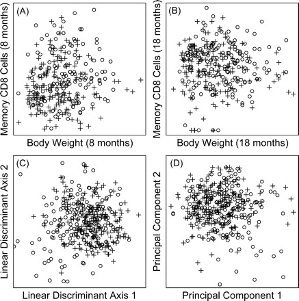
Overlap between short- and long-lived life-span quartiles. In each plot, open circles (○) represent mice associated with the shortest-lived quartile, whereas plus signs (+) represent mice associated with the longest-lived quartile. A and B, Quartile relationships with respect to body weight and the CD8M T-cell subset at 8 and 18 months of age, respectively. C, All mice in the data set plotted with respect to two linear discriminant axes, which were derived from the 29 continuous predictor variables listed in Table 1. D, Mice plotted with respect to the first two principal components derived from the 29 continuous predictor variables. The two principal components account for 6.8% of the total variation among the 29 variables

Comparison of Machine Learning Algorithms

Predictive models were constructed using each of 22 machine learning algorithms (Table 2). For each algorithm, models were generated using all 31 predictor variables, as well as subsets of 12 and 6 predictor variables that were chosen by ranking variables according to their importance to prediction accuracy based on the Random Forest algorithm (33) (see Figure 3). This algorithm generates a useful measure of variable importance based on cross-validation and the accuracy decline that results when predictors are removed from the data set (44). We used this measure to rank all 31 predictor variables in terms of their importance for predicting life-span quartile (Figure 3). This approach suggested that the subset CD4V_18 and body weight measurements were the most important variables for life-span quartile prediction, whereas some variables, such as T4_4, T4_15, and LEP_15, may have a net deleterious effect on prediction accuracy. These results were supported by our evaluation of algorithm performance (Table 2), because most algorithms performed best when only the 12 or 6 most important predictors were used (Table 2). For instance, using all 31 predictor variables, SVM predicted life-span quartile with 29.90% accuracy, but this value increased to 34.03% when only the best 12 predictor variables were used.

Figure 3.

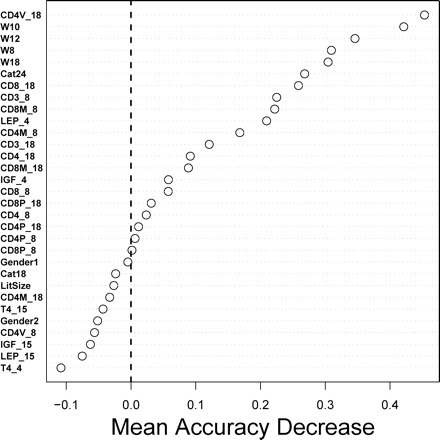
Random Forest evaluation of variable importance. Variables listed near the top of the figure are most important for prediction of life-span quartile. The Random Forest algorithm constructs a “forest” of decision trees, where each tree generates predictions based on a randomly chosen set of predictor variables. Predictions are then generated by majority vote among all trees in the forest (33). For the 741 mice we considered, the algorithm generates forests using a bootstrap sample of approximately 500 mice; remaining mice are used as an internal testing set for accuracy evaluation. For a given predictor X, predictive accuracy is evaluated before and after permuting values of X among mice. The difference between the two obtained accuracies is then determined and used as a measure of variable importance. This procedure was repeated 10,000 times using forests of 2000 decision trees per trial. The figure shows the average accuracy change among all 10,000 trials

All algorithms predicted life-span quartile with accuracy significantly greater than that expected by random guessing (25%), and in some cases, simple approaches performed as well as highly complex methods (Table 2). Regression-based approaches, which have been used previously to generate life-span–predictive models [e.g., (8,9,11)], performed well in some cases (31.8% accuracy), but were not among the best performing algorithms (see Table 2; multinomial logistic regression and simple linear regression). Overall, three algorithms emerged as the most promising (NSC, SVM, and Stabilized Linear Discriminant Analysis [SLDA]). SVM and SLDA obtained a maximal accuracy of 34.03% and 34.06%, respectively, using the 12 most important predictor variables (Table 2). The NSC algorithm, however, attained slightly greater accuracy using only six predictors (34.37%).

The NSC Algorithm: Variable Selection

Further experiments were performed to determine whether NSC could attain greater accuracy using more than six predictors or attain a similar level of accuracy with fewer predictors. An initial model was constructed by using only the two most important predictors (CD4V_18 and W10), which yielded an average accuracy of 33.1%. Variables were then added individually according to their importance (Figure 3). We found that accuracy peaked at 34.5% following the addition of five predictor variables (CD4V_18, W8, W10, W12, and W18) (Figure 4). This analysis suggested that strong performance could be attained using a relatively small number of predictor variables.

Figure 4.

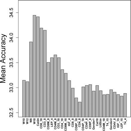
Variable subset evaluation. Prediction accuracy was evaluated for different variable subsets using the Nearest Shrunken Centroid algorithm. Variables were entered into the model according to their importance, as indicated by results shown in 
 Figure 3. The first model included variables CD4V_18 and W10 as life-span predictors. The accuracy obtained using this model was evaluated by 10-fold cross-validation and 10,000 simulations. The average accuracy among all simulations is represented by the leftmost bar. Each subsequent bar from left to right indicates the accuracy obtained by adding the next most important variable to the model. The rightmost bar represents the mean accuracy obtained using the full model with all 31 predictor variables

We evaluated the prediction accuracy attained by the NSC algorithm using each of the ₃₁C₂ = 465 possible predictor variable pairs (at least 100 cross-validation simulations were performed per pair). This analysis indicated that CD4V_18 and W18 provided the best two-variable subset, which yielded a prediction accuracy of 33.5%. The second best two-variable subset provided 33.4% accuracy and also included CD4V_18, but in combination with another T-cell measure (CD8M_8) rather than a body weight variable. We next evaluated each of the ₃₁C₃ = 4495 three-variable subsets (using at least 20 simulations per subset) and found that best performance was attained with CD4V_18, W8, and W18 as predictors (34.4%). Taken together, these results suggested that the best four-variable subset would include CD4V_18. We thus evaluated the ₃₀C₃ = 4060 possible four-variable subsets that include CD4V_18 and found that a subset of CD4V_18, W8, W10, and W18 yielded an accuracy of 34.6%. Continuing in this fashion, we examined the ₂₉C₃ = 3654 possible five-variable subsets that include CD4V_18 and W18. This analysis suggested a five-variable model with three body weight variables (W8, W10, and W18) and two T-cell subset variables (CD4V_18 and CD4M_8), which yielded an accuracy of 35.3% (95% CI, 35.2%-35.4%). This was the best overall performance in our analysis, as further exhaustive searches did not identify a six-variable model with significantly improved accuracy. We also found that inclusion of principal components that combined data from multiple weight measures or related sets of T-cell subsets did not improve the accuracy of the model. The performance of our best overall predictive model is illustrated by Figure 5, which displays the distribution of accuracies obtained among 10,000 cross-validation simulations, and provides a comparison to the distribution of accuracies obtained by an algorithm that generates predictions randomly.

Figure 5.

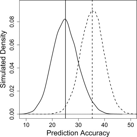
Simulation results. The Nearest Shrunken Centroid (NSC) algorithm was implemented using five predictor variables (CD4M_8, CD4V_18, W8, W10, and W18). The plot shows the distribution of accuracies obtained on the testing set among 10,000 simulation trials. Solid line: Accuracy distribution obtained by a random guessing algorithm. Dotted line: Accuracy distribution obtained by the NSC algorithm. Solid vertical line: Mean accuracy among all trials for the random guessing algorithm (approximately 25%). Dotted vertical line: Mean accuracy among all trials for the NSC algorithm (35.3%)

The NSC Algorithm: Additional Analyses

The five-variable prediction model we developed was used to separate mice into groups that, based on five variables measured before 2 years of age, are projected to be either shorter or longer lived. For each of the 741 mice considered in our analysis, a predicted life-span quartile was generated based on all other 740 mice (leave-one-out cross-validation). We then evaluated mice assigned to the two shorter-lived life-span quartiles as compared to the two longer-lived quartiles. Mice projected to be longer-lived had a mean life span of 930.6 days, whereas mice projected to be shorter-lived had a mean life span of 879.5 days. Survivorship curves associated with these two groups were significantly different from each other (p <.0001; log-rank test) (see Figure 6), and mice projected to be longer-lived had age-specific mortality rates reduced significantly by 36.9% (95% CI, 26.8%–45.7%) (p <.0001; proportional hazards model).

Figure 6.

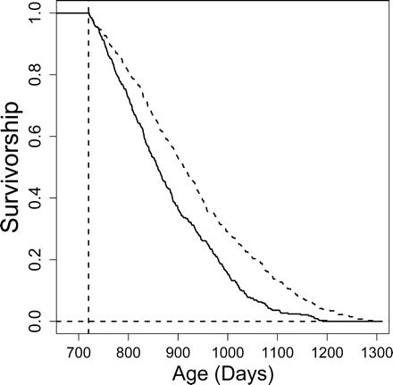
Predicted life span and survivorship. The life span of each mouse in the data set was predicted using the Nearest Shrunken Centroid and the leave-one-out method (see text). Five predictors were used in the model (CD4M_8, CD4V_18, W8, W10, and W18). Dotted line: Cohort of mice with predicted life span in the upper two quartiles. Solid line: Cohort of mice with predicted life span in the lower two quartiles. Dotted vertical line: Minimum life span of mice that were included in the analysis (720 days). Zero survivorship is indicated by the dotted horizontal line.

Mice projected to be longer-lived also had significantly greater maximum life span, using survival to the pooled 90th percentile as a criterion for extreme longevity. Among all mice, the 90th percentile life span was 1087 days, and whereas only 3.6% of mice projected to be shorter-lived survived this long, we found that 15.0% of mice assigned to the longer-lived group survived this time period (χ² = 26.45; p <.0001).

The estimated probability of a mouse belonging to quartile x given its scores on a number of variables is referred to as posterior class probability (20). Posterior class probabilities are generated by many machine learning methods and provide a useful form of continuous output. Such output represents an integration of potentially many predictor variables and, in the present context, can be used to construct an index associated with life span. Using the leave-one-out method described above, we calculated the posterior probability of belonging to the longest-lived quartile for each of the 741 mice considered in our analysis, based on the NSC algorithm and the probabilistic framework developed by Tibshirani and colleagues (29). This approach provided an index that was significantly associated with life span (r = 0.15, p <.001) (Figure 7). Likewise, we calculated the posterior probability of belonging to the shortest-lived quartile for each mouse, which provided an index exhibiting the opposite pattern of association with life span (r = −0.14; p <.001). These associations were not dependent on outlying observations, because the same trends were identified based on the Spearman rank correlation (|r_s| > 0.14, p <.001).

Figure 7.

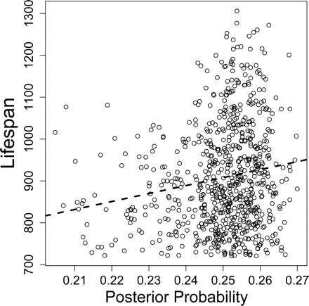
Posterior probability and life span. The posterior probability of belonging to the longest-lived quartile was determined for each mouse in the data set using the leave-one-out method (see text). Five predictors were used in the model (CD4M_8, CD4V_18, W8, W10, and W18). Dotted line: Least-squares regression line

Prediction accuracy increases systematically as more training examples are used during the algorithm learning phase. At some point, however, additional training examples provide only negligible returns in predictive accuracy. In our analysis, training was performed with randomly sampled sets of 664 mice (90% of all mice that met our inclusion criteria). To determine whether this training set size exceeds a point of diminishing returns, we varied the number of training examples between 76 and 664 mice, and used cross-validation to evaluate predictive accuracy for each number of training examples (using NSC and the five-variable model mentioned above). Accuracy gains due to increased training set size diminished slightly beyond 400 training samples (Figure 8). A moving average time series model was used to forecast the accuracy expected for 1000 training examples, based on the observed increase in accuracy between 76 and 664 training examples. This analysis indicated that, based on the set of five predictors from which our best model was developed, 1000 training samples would yield an average accuracy of 40.0% (± 1.2%) (Figure 8).

Figure 8.

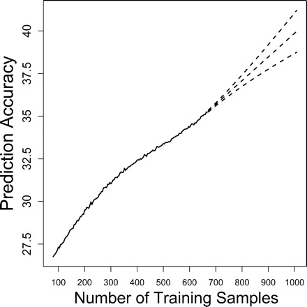
Effect of training set size on accuracy. The number of training samples was varied between 10% and 90% of the total data set (between 75 and 667 mice). For each training set size, the mean accuracy obtained by the Nearest Shrunken Centroid algorithm was determined by 10,000 simulations (using 10-fold cross-validation). The mean accuracies obtained for each training set size are indicated by the solid line. Dashed lines: Forecasted accuracy for larger training set sizes (between 667 and 1000 mice). Middle dashed line: Forecasted accuracy. Top and bottom dashed lines: Standard error margins. Forecasts were generated using a moving average model with two parameters and two degrees of differencing. Model selection was based on the Akaike Information Criterion described by Brockwell and Davis (72)

Discussion

Models that predict individual life span can provide a valuable tool for aging research, and development of such models represents a platform for understanding relationships between longevity and other phenotypic characteristics. Full-length survivorship experiments require years to complete and are a rate-limiting step in the study of mammalian aging. Clearly, such experiments will never be replaced by predictive models. Well-developed models, however, can generate preliminary data years in advance, and the output of such models, as an integration of multiple variables that may predict life span individually, can provide a surrogate target for aging research that is easier to evaluate than life span. Indeed, a similar concept has already been successfully applied using the Drosophila model system (45). Using gene expression patterns that predict life span, Baur and colleagues (45) developed a survivorship screen that satisfactorily revealed the known effects of temperature, caloric restriction, and resveratrol on Drosophila life span, but required 80% less time than a full-length survivorship study. We have here explored the plausibility of such a model in mice, and our results provide a realistic indication of how accurately mouse life span can be predicted using state-of-the-art machine learning algorithms. Using a set of physiological measurements made prior to 24 months of age, we have shown that mouse life-span quartile can be predicted with an average accuracy of 35.3%. This estimate is based on a stringent cross-validation criterion, in which accuracy is based on prediction of test cases not used in model construction. We suggest that considerable potential remains for improving on the 35.3% prediction accuracy attained in this study. Development of new computational approaches, generation of larger data sets, and identification of candidate predictor variables are all avenues by which our result can be improved.

Machine learning approaches vary considerably in terms of their complexity, performance on easy versus difficult tasks, and the ease with which investigators can apply these methods. We have carried out a performance evaluation of many machine learning approaches for the specific task of predicting mouse life span, which provides guidance for future studies addressing this issue. It should be borne in mind that, for any algorithm, performance is data-dependent and will vary across contexts. It is therefore impossible and incorrect to identify a single “best algorithm” that will always yield the best predictive performance (20). We anticipate, however, that any survivorship data set containing life-span-predictor variables will share some properties with data analyzed here. For instance, some level of “overlap” between mice belonging to different life-span quartiles seems inevitable, such that accurate predictions will require recognition of complex decision boundaries (see Figures 1 and 2). The best algorithms identified in our analysis were most successful at characterizing such decision boundaries, and therefore provide good starting points for future investigations aimed at prediction of mouse life span. We found that life span was accurately predicted by SVM and SLDA algorithms, but that the NSC approach provided the best overall performance. This algorithm was developed in the context of DNA microarray data sets and was used to classify cancer subtypes based on gene expression patterns (29). The approach is also straightforward to implement and can be understood by nonexperts. It is computationally inexpensive, as 10,000 simulations can be carried out in <1 hour on a standard desktop PC; other algorithms listed in Table 2 required as much as 2 days for execution using the same hardware. The method is similar to the Nearest Centroid approach, which uses p predictor variables to obtain a p-dimensional centroid for each life-span quartile, and predicts life-span quartile for new cases by determining which centroid the test case is most similar to. In the NSC approach, however, class centroids are standardized and “shrunk” toward an overall centroid (calculated by averaging centroids among life-span quartiles), which has the effect of emphasizing those predictors with low levels of variation in each class (see 29). This yields a classification rule characterized by complex, nonlinear decision boundaries, which has been found to perform well on challenging machine learning tasks (29,46).

The performance of machine learning approaches can generally be improved by providing a larger number of training samples during the algorithm learning stage. Numerous sources of variation obscure relationships that exist between life-span quartile and the predictor variables we measured. To deal with this variation, effective algorithms must accurately characterize underlying biological relationships, and must do this consistently despite “noise” that obscures underlying relationships. In other words, for accurate prediction, decision boundaries chosen by algorithms should be unbiased but, at the same time, must be robust to noise and chance variation within training data. In general, these aspects of predictive modeling are in tension but, by increasing the number of training samples for algorithm learning, it is often possible to decrease both the bias and variance associated with decision boundaries (20). Our study evaluated models based on 664 training samples, which is small compared to training set sizes commonly used for machine learning tasks. In the context of handwritten digit recognition, for instance, benchmark tasks commonly include more than 50,000 training samples (21,47). We therefore expect that the generation of larger data sets would lead to further improvements in life-span prediction accuracy. We achieved 35.3% prediction accuracy using 664 training samples, but our analyses indicate that 1000 training samples would yield an accuracy of approximately 40% (Figure 8) with the same, limited set of predictors. This finding suggests that a survivorship experiment generating 1000 mice (living beyond 2 years of age) would provide a more useful model than that developed in this study. Even larger experiments could only improve predictive accuracy but risk low returns in exchange for substantial efforts and costs.

The successful prediction of mouse life span ultimately depends on the quality of predictor variables that are available. Predictor variables, or some multivariate combination of predictors, must have a linear or nonlinear association with life span. Otherwise, a useful model cannot be constructed, regardless of the computational approach that is taken. The basis of associations between predictors and life span is of special interest. Predictor variables can be associated with life span through a specific disease process. For example, if leukemia is a major factor contributing to mortality in a cohort, blood cell counts may provide an effective predictor of longevity, and the overall predictive model will be uninformative with regard to aging mechanisms. Alternatively, predictor variables can be associated with life span because they characterize some aspect of the aging process. We found, for example, that body weight measurements between 8 and 18 months of age were among the most important predictors of life-span quartile, and that four of the top five predictors were body weight variables. These results are consistent with our findings from earlier studies (8,11), as well as from multiple investigations showing that, within individual species, lower body weight is commonly associated with increased longevity (48–50). Links between body weight, aging, and longevity are not fully understood, but the GH/IGF-I axis may be an underlying explanatory factor (12). In fact, we found that, among mice living beyond 2 years of age, body weight values were correlated with serum IGF-I levels at 4 and 15 months of age (0.42 < r < 0.46). In some segregating mouse populations, low IGF-I levels early in life do indeed predict longer life span (51).

Identification of new phenotypic traits that predict life span may be the most promising approach for improving on our results. We examined 31 predictor variables, but life span was most accurately forecasted when only the five strongest predictors were used in model construction. The strongest predictors in our current data set are drawn from two physiological domains, body weight and T-cell biology, and there are strong correlations among the various body weight measures as well as among the T-cell subset frequencies. Including several measures of weight, or several measures of T-cell status, may improve the performance of these predictive algorithms by diminishing the variation reflecting measurement error or day-to-day variations in biological state that are independent of inter-individual differences (for example, the effects of a recent meal or hydration state on measured body weight). We suspect that incorporation of measures drawn from other physiological domains, such as tests of motor function, cognitive function, or resistance to DNA damage, might be a useful step toward improved predictive performance. Previous studies, for example, have identified other noninvasive phenotypic traits (correlated with life span) that were not evaluated in our study. Harrison and Archer (2), for example, showed that tight wire clinging ability, open field activity, collagen denaturation rate, hair regrowth, wound healing, and blood hemoglobin concentration were all correlated with longevity in certain mouse genotypes. Flurkey and colleagues (15) described several other potentially useful phenotypic traits, such as urine concentrating ability and carbon dioxide production, for which relationships with longevity have not been examined. A nearly endless list of possible predictor variables is provided by expression measures of individual genes or composite measures derived from a number of genes. In skin tissue, for instance, p16^INK4A has been found to correlate with chronological age, although its value as a predictor of longevity has not been previously considered (52,53). Some gene expression variables may reflect certain physiological states beneficial for longevity, and may therefore prove to be unexpectedly valuable longevity predictors, even when population-level variation is attributable to nongenetic or “chance” sources in uniform environments [e.g., (54)]. For genetically heterogeneous populations, such as that considered in the present study, genetic polymorphisms represent an especially important avenue for investigation. Various forms of genetic data, such as single nucleotide polymorphisms, could readily be incorporated into models as categorical predictor variables, which may improve prediction accuracy by accounting for interactions between genotypic and phenotypic characters. Such interactions may be of considerable importance, as Harrison and Archer (2) found that relationships between phenotypic traits and longevity were often dependent on genotype.

The methods used in the present study also provide a useful framework for investigations aimed at discovering and validating biomarkers of aging. Aging biomarkers provide an operational definition of aging that is useful for testing hypotheses about aging experimentally, such as whether aging is delayed by mutations or environmental interventions (15). The denaturation rate of collagen, for example, has been used as a biomarker to suggest that aging is delayed in long-lived mouse strains (55). The quest for aging biomarkers has been controversial, and hindered by both conceptual and methodological hurdles, including disagreement regarding the definition of “biomarker,” overlap between aging and disease processes, and lack of knowledge about aging mechanisms (56–59). For example, there is an important conceptual distinction between predictors of life span and biomarkers of aging. To be useful as a biomarker of aging, a measurement must be able to distinguish among individuals who are aging at different rates—for example, because of differential exposure to a putative anti-aging intervention. Conceptually, such traits must be measured in individuals who have already experienced some effects of the aging process—for example, middle-aged adults. Inherited alleles, or weight at birth, for example, may prove to be a strong predictor of life span or of other age-related end points, and yet have no value as a measure of the rate at which aging has occurred in a specific individual.

Nevertheless, predictive capacity is an important component of biomarker validation, and it is widely agreed that legitimate biomarkers must predict the outcome of a wide range of age-sensitive events in different physiological systems and, ultimately, should be predictive of individual life span (2,4,60–63). The cross-validation strategy used in the present study, involving random division of data into training and testing sets, provides a useful way of evaluating predictive capacity and thus provides a framework for biomarker validation. Furthermore, we have used machine learning to generate posterior class probabilities for different life-span quartiles (see Figure 7). Such posterior probabilities may provide useful indices that serve as biomarkers or as indicators of “biological age” (64–66). A key advantage of this approach is that alternative models used to generate posterior probabilities can be compared based on cross-validation life-span prediction accuracy. This could make progress stemming from the biomarker research agenda more transparent from skeptical viewpoints because, for example, it would be unambiguous to determine whether an index generated by predictors X, Y, and Z is superior to an index generated by predictors P, Q, and S.

The model we developed predicts life-span quartile with 35.3% accuracy, and we have shown that this model can assign mice to groups that differ in mean life span by 5.8% (930.6 vs 879.5 days; see Figure 6). At a glance, this 5.8% difference seems minor. It should be noted, however, that an algorithm predicting death from cancer in the American population (with 100% accuracy) would separate humans into groups differing by <3% in mean life span (67). We therefore suggest that our model provides informative predictions with biologically meaningful underpinnings. Furthermore, we are optimistic that more accurate life-span-predictive models can be formulated in future investigations. The computational approach that performed best in our analysis was developed within the last decade (29). In the coming decade, intensive research efforts will focus on improving variable selection methods (68), extracting informative features from a set of variables (69), developing ensemble approaches for combining outputs of multiple algorithms (70), and filtering training samples to identify maximally informative cases for learning (71). Such investigations will lay the groundwork for development of new algorithms, which can be complemented by better understanding of aging mechanisms and exploitation of life span predictors at the molecular and phenotypic levels. These approaches, both computational and biological, can improve the accuracy with which mouse life span is predicted, and should advance interdisciplinary approaches to biogerontology and the study of mammalian aging.

References

- 1.Botwinick J, West R, Storandt M. Predicting death from behavioral test performance. J Gerontol. 1983;33:755-762. [DOI] [PubMed] [Google Scholar]
- 2.Harrison DE, Archer JR. Biomarkers of aging: tissue markers. Future research needs, strategies, directions and priorities. Exp Gerontol. 1988;23:309-321. [DOI] [PubMed] [Google Scholar]
- 3.Reynolds MA, Ingram DK, Talan M. Relationship of body temperature stability to mortality in aging mice. Mech Ageing Dev. 1985;30:143-152. [DOI] [PubMed] [Google Scholar]
- 4.Ingram DK, Reynolds MA. Assessing the predictive validity of psychomotor tests as measures of biological age in mice. Exp Aging Res. 1986;12:155-162. [DOI] [PubMed] [Google Scholar]
- 5.Miller RA, Chrisp C, Galecki A. CD4 memory T cell levels predict lifespan in genetically heterogenous mice. FASEB J. 1997;11:775-783. [DOI] [PubMed] [Google Scholar]
- 6.Miller RA. Biomarkers of aging: prediction of longevity by using age-sensitive T-cell subset determinations in a middle-aged, genetically heterogeneous mouse population. J Gerontol Biol Sci. 2001;56A:B180-B186. [DOI] [PMC free article] [PubMed] [Google Scholar]
- 7.Miller RA, Chrisp C. T cell subset patterns that predict resistance to spontaneous lymphoma, mammary adenocarcinoma, and fibrosarcoma in mice. J Immunol. 2002;169:1619-1625. [DOI] [PubMed] [Google Scholar]
- 8.Miller RA, Harper JM, Galecki A, Burke D. Big mice die young: early life body weight predicts longevity in genetically heterogeneous mice. Aging Cell. 2002;1:22-29. [DOI] [PubMed] [Google Scholar]
- 9.Harper JM, Wolf N, Galecki AT, Pinkosky SL, Miller RA. Hormone levels and cataract scores as sex-specific, mid-life predictors of longevity in genetically heterogeneous mice. Mech Ageing Dev. 2003;124:801-810. [DOI] [PubMed] [Google Scholar]
- 10.Anisimov VN, Arbeev KG, Popovich IG, Zabezhinksi MA, Arbeeva LS, Yashin AI. Is early life body weight a predictor of longevity and tumor risk in rats? Exp Gerontol. 2004;39:807-816. [DOI] [PubMed] [Google Scholar]
- 11.Harper JM, Galecki AT, Burke DT, Miller RA. Body weight, hormones and T cell subsets as predictors of life span in genetically heterogeneous mice. Mech Ageing Dev. 2004;125:381-390. [DOI] [PubMed] [Google Scholar]
- 12.Miller RA, Austad S. Why do big dogs die young? In: Masaro E, Austad S, eds. Handbook of the Biology of Aging. San Diego, CA: Academic Press; 2005:512–533.
- 13.Ramsey JJ, Colman RJ, Binkley NC, et al. Dietary restriction and aging in rhesus monkeys: the University of Wisconsin study. Exp Gerontol. 2000;35:1131-1149. [DOI] [PubMed] [Google Scholar]
- 14.Mattison JA, Lane MA, Roth GS, Ingram DK. Caloric restriction in rhesus monkeys. Exp Gerontol. 2003;38:35-46. [DOI] [PubMed] [Google Scholar]
- 15.Flurkey K, Currer JM, Harrison DE. The mouse in aging research. In: Fox JG, Barthold S, Davisson M, Newcomer CE, Quimby FW, Smith A, eds. The Mouse in Biomedical Research, Volume 3. Burlington, MA: Elsevier; 2007:637–672.
- 16.Vieira C, Pasyukova EG, Zeng ZB, Hackett JB, Lyman RF, Mackay TF. Genotype-environment interaction for quantitative trait loci affecting life span in Drosophila melanogaster Genetics. 2000;154:213-227. [DOI] [PMC free article] [PubMed] [Google Scholar]
- 17.Vermeulen CJ, Bijlsma R. Changes in mortality patterns and temperature dependence of lifespan in Drosophila melanogaster caused by inbreeding. Heredity. 2004;92:275-281. [DOI] [PubMed] [Google Scholar]
- 18.Swindell WR, Bouzat JL. Inbreeding depression and male survivorship in Drosophila: implications for senescence theory. Genetics. 2006;172:317-327. [DOI] [PMC free article] [PubMed] [Google Scholar]
- 19.Neter J, Kutner MH, Nachtsheim CJ, Wasserman W. Applied Linear Regression Models. Chicago, IL: McGraw-Hill; 1996.
- 20.Duda RO, Hart PE, Stork DG. Pattern Classification. 2nd Ed. New York: John Wiley and Sons; 2001.
- 21.Liu CL, Nakashima K, Sako H, Fujisawa H. Handwritten digit recognition: benchmarking of state-of-the-art techniques. Pattern Recognit. 2003;36:2271-2285. [Google Scholar]
- 22.Teow LN, Loe KF. Robust vision-based features and classification schemes for off-line handwritten digit recognition. Pattern Recognit. 2002;35:2355-2364. [Google Scholar]
- 23.Andorf C, Dobbs D, Honavar V. Exploring inconsistencies in genome-wide protein function annotations: a machine-learning approach. BMC Bioinformatics. 2007;8:284. [DOI] [PMC free article] [PubMed] [Google Scholar]
- 24.Li S, Shi F, Pu F, et al. Hippocampal shape analysis of Alzheimer disease based on machine learning methods. Am J Neuroradiol. 2007;28:1339-1345. [DOI] [PMC free article] [PubMed] [Google Scholar]
- 25.Zernov VV, Balakin KV, Ivaschenko AA, Savchuk NP, Pletnev IV. Drug discovery using support vector machines. The case studies of drug-likeness, agrochemical-likeness, and enzyme inhibition predictions. J Chem Inf Comput Sci. 2003;43:2048-2056. [DOI] [PubMed] [Google Scholar]
- 26.Fox T, Kriegl JM. Machine learning techniques for in silico modeling of drug metabolism. Curr Top Med Chem. 2006;6:1579-1591. [DOI] [PubMed] [Google Scholar]
- 27.Miller RA, Austad S, Burke D, et al. Exotic mice as models for aging research: polemic and prospectus. Neurobiol Aging. 1999;20:217-231. [DOI] [PubMed] [Google Scholar]
- 28.Troyanskaya O, Cantor M, Sherlock G, et al. Missing value estimation methods for DNA microarrays. Bioinformatics. 2001;17:520-525. [DOI] [PubMed] [Google Scholar]
- 29.Tibshirani R, Hastie T, Narasimhan B, Chu G. Diagnosis of multiple cancer types by shrunken centroids of gene expression. Proc Natl Acad Sci U S A. 2002;99:6567-6572. [DOI] [PMC free article] [PubMed] [Google Scholar]
- 30.Laeuter J, Glimm E, Kropf S. Multivariate tests based on left-spherically distributed linear scores. Ann Stat. 1998;26:1972-1988. [Google Scholar]
- 31.Byvatov E, Schneider G. Support vector machine applications in bioinformatics. Appl Bioinformatics. 2003;2:67-77. [PubMed] [Google Scholar]
- 32.Williams CKI, Barber D. Bayesian classification with Gaussian processes. IEEE Trans Pattern Anal Mach Intell. 1998;20:1342-1351. [Google Scholar]
- 33.Breiman L. Random forests. Mach Learn. 2001;45:5-32. [Google Scholar]
- 34.Platt JC. Fast training of support vector machines using sequential minimal optimization. In: Schoelkopf C, Burges C, Smola A, eds. Advances in Kernal Methods–Support Vector Learning. Cambridge, MA: MIT Press; 1998:185–208.
- 35.Tutz G, Binder H. Localized classification. Statistics and Computing. 2005;15:155-166. [Google Scholar]
- 36.Lee EK, Cook D, Klinke S, Lumley T. Projection pursuit for exploratory supervised classification. J Comput Graph Stat. 2005;14:831-846. [Google Scholar]
- 37.le Cessie S, van Houwelingen JC. Ridge estimators in logistic regression. Appl Stat. 1992;41:191-201. [Google Scholar]
- 38.Basheer IA, Hajmeer M. Artificial neural networks: fundamentals, computing, design, and application. J Microbiol Methods. 2000;43:3-31. [DOI] [PubMed] [Google Scholar]
- 39.Hothorn T, Hornik K, Zeileis A. Unbiased recursive partitioning: a conditional inference framework. J Comput Graph Stat. 2006;15:651-674. [Google Scholar]
- 40.Patrick EA, Fischer FP. A generalized k-nearest neighbor rule. Information and Control 1970;16:128-152. [Google Scholar]
- 41.Quinlan R. C4.5: Programs for Machine Learning. San Diego, CA: Morgan Kaufmann; 1993.
- 42.Frank E, Witten IH. Generating accurate rule sets without global optimization. In: Shavlik J, ed. Machine Learning: Proceedings of the Fifteenth International Conference. San Francisco, CA: Morgan Kaufmann Publishers; 1998:144–151.
- 43.Cohen WW. Fast effective rule induction. In: Proceedings of the 12th International Conference on Machine Learning. Lake Tahoe, CA: Morgan Kaufmann; 1995:115–123.
- 44.Diaz-Uriarte R, Alvarez de Andrés S. Gene selection and classification of microarray data using random forest. BMC Bioinformatics. 2006;7:3. [DOI] [PMC free article] [PubMed] [Google Scholar]
- 45.Bauer JH, Goupil S, Garber GB, Helfand SL. An accelerated assay for the identification of lifespan-extending interventions in Drosophila melanogaster Proc Natl Acad Sci U S A. 2004;101:12980-12985. [DOI] [PMC free article] [PubMed] [Google Scholar]
- 46.Sharma P, Sahni NS, Tibshirani R, et al. Early detection of breast cancer based on gene-expression patterns in peripheral blood cells. Breast Cancer Res. 2005;7:R634-R644. [DOI] [PMC free article] [PubMed] [Google Scholar]
- 47.Liu CL, Sako H. Class-specific feature polynomial classifier for pattern classification and its application to handwritten numeral recognition. Pattern Recognit. 2006;39:669-681. [Google Scholar]
- 48.Patronek GJ, Waters DJ, Glickman LT. Comparative longevity of pet dogs and humans: implications for gerontology research. J Gerontol Biol Sci. 1997;52A:B171-B178. [DOI] [PubMed] [Google Scholar]
- 49.Speakman JR, van Acker A, Harper EJ. Age-related changes in the metabolism and body composition of three dog breeds and their relationship to life expectancy. Aging Cell. 2003;2:265-275. [DOI] [PubMed] [Google Scholar]
- 50.Greer KA, Canterberry SC, Murphy KE. Statistical analysis regarding the effects of height and weight on life span of the domestic dog. Res Vet Sci. 2007;82:208-214. [DOI] [PubMed] [Google Scholar]
- 51.Harper JM, Durkee R, Dysko C, Austad SN, Miller RA. Genetic modulation of hormone levels and life span in hybrids between laboratory and wild-derived mice. J Gerontol A Biol Sci Med Sci. 2006;61:1019-1029. [DOI] [PMC free article] [PubMed] [Google Scholar]
- 52.Sharpless NE. Ink4a/Arf links senescence and aging. Exp Gerontol. 2004;39:1751-1759. [DOI] [PubMed] [Google Scholar]
- 53.Ressler S, Bartkova J, Niederegger H, et al. p16ink4a is a robust in vivo biomarker of cellular aging in human skin. Aging Cell. 2006;5:379-389. [DOI] [PubMed] [Google Scholar]
- 54.Rea SL, Wu D, Cypser JR, Vaupel JW, Johnson TE. A stress-sensitive reporter predicts longevity in isogenic populations of Ceanorhabditis elegans Nat Genet. 2005;37:894-898. [DOI] [PMC free article] [PubMed] [Google Scholar]
- 55.Flurkey K, Papaconstantinou J, Miller RA, Harrison DE. Lifespan extension and delayed immune and collagen aging in mutant mice with defects in growth hormone production. Proc Natl Acad Sci U S A. 2001;98:6736-6741. [DOI] [PMC free article] [PubMed] [Google Scholar]
- 56.Costa PT, McCrae RR. Concepts of functional or biological age: a critical view. In: Andres R, Bierman EL, Hazzard WR, eds. Principles of Geriatric Medicine. New York: McGraw Hill; 1985:30–37.
- 57.Adelman RC. Biomarkers of aging. Exp Gerontol. 1987;22:227-229. [DOI] [PubMed] [Google Scholar]
- 58.Costa PT, McCrae RR. Measures and markers of biological aging: “a great clamoring…of fleeting significance.”. Arch Gerontol Geriat. 1988;7:211-214. [DOI] [PubMed] [Google Scholar]
- 59.Miller RA. Biomarkers of aging. Sci Aging Knowledge Environ. 2001;1:pe2. [DOI] [PubMed] [Google Scholar]
- 60.Harrison DE, Archer JR. Physiological assays for biological age in mice: relationship to collagen, renal function, and longevity. Exp Aging Res. 1983;9:245-251. [DOI] [PubMed] [Google Scholar]
- 61.Ingram DK. Toward the behavioral assessment of biological aging in the laboratory mouse: concepts, terminology, and objectives. Exp Aging Res. 1983;9:225-238. [DOI] [PubMed] [Google Scholar]
- 62.Ingram DK. Key questions in developing biomarkers of aging. Exp Gerontol. 1988;23:429-434. [DOI] [PubMed] [Google Scholar]
- 63.Butler RN, Sprott R, Warner H, et al. Biomarkers of aging: from primitive organisms to humans. J Gerontol A Biol Sci Med Sci. 2004;59:560-567. [DOI] [PubMed] [Google Scholar]
- 64.Bowden DM, Short RA, Williams DD. Constructing an instrument to measure the rate of aging in female pigtailed macaques (Macaca nemestrina). J Gerontol Biol Sci. 1990;45A:B59-B66. [DOI] [PubMed] [Google Scholar]
- 65.Nakamura E, Miyao K. Further evaluation of the basic nature of the human biological aging process based on a factor analysis of age-related physiological variables. J Gerontol A Biol Sci Med Sci. 2003;58:196-204. [DOI] [PubMed] [Google Scholar]
- 66.Nakamura E, Miyao K. A method for identifying biomarkers of aging and constructing an index of biological age in humans. J Gerontol A Biol Sci Med Sci. 2007;62:1096-1105. [DOI] [PubMed] [Google Scholar]
- 67.Olshansky SJ, Carnes BA, Cassel C. In search of Methuselah: estimating the upper limits to human longevity. Science. 1990;250:634-640. [DOI] [PubMed] [Google Scholar]
- 68.Gadat S, Younes L. A stochastic algorithm for feature selection in pattern recognition. J Mach Learn Res. 2007;8:509-547. [Google Scholar]
- 69.Arriaga RI, Vempala S. An algorithmic theory of learning: robust concepts and random projection. Mach Learn. 2006;63:161-182. [Google Scholar]
- 70.Zhang P, Bui TD, Suen CY. A novel cascade ensemble classifier system with a high recognition performance on handwritten digits. Pattern Recognit. 2007;40:3415-3429. [Google Scholar]
- 71.Li Y, de Ridder D, Duin RPW, Reinders MJT. Integration of prior knowledge of measurement noise in kernel density classification. Pattern Recognit. 2008;41:320-330. [Google Scholar]
- 72.Brockwell PJ, Davis RA. Introduction to Time Series and Forecasting. 2nd Ed. New York: Springer; 2002.