Noise Correlations in Cortical Area MT and Their Potential Impact on Trial-by-Trial Variation in the Direction and Speed of Smooth-Pursuit Eye Movements

Xin Huang; Stephen G Lisberger

doi:10.1152/jn.00010.2009

. 2009 Mar 25;101(6):3012–3030. doi: 10.1152/jn.00010.2009

Noise Correlations in Cortical Area MT and Their Potential Impact on Trial-by-Trial Variation in the Direction and Speed of Smooth-Pursuit Eye Movements

Xin Huang ¹, Stephen G Lisberger ¹

PMCID: PMC2694100 PMID: 19321645

Abstract

Smooth-pursuit eye movements are variable, even when the same tracking target motion is repeated many times. We asked whether variation in pursuit could arise from noise in the response of visual motion neurons in the middle temporal visual area (MT). In physiological experiments, we evaluated the mean, variance, and trial-by-trial correlation in the spike counts of pairs of simultaneously recorded MT neurons. The correlations between responses of pairs of MT neurons are highly significant and are stronger when the two neurons in a pair have similar preferred speeds, directions, or receptive field locations. Spike count correlation persists when the same exact stimulus form is repeatedly presented. Spike count correlations increase as the analysis window increases because of correlations in the responses of individual neurons across time. Spike count correlations are highest at speeds below the preferred speeds of the neuron pair and increase as the contrast of a square-wave grating is decreased. In computational analyses, we evaluated whether the correlations and variation across the population response in MT could drive the observed behavioral variation in pursuit direction and speed. We created model population responses that mimicked the mean and variance of MT neural responses as well as the observed structure and amplitude of noise correlations between pairs of neurons. A vector-averaging decoding computation revealed that the observed variation in pursuit could arise from the MT population response, without postulating other sources of motor variation.

INTRODUCTION

Visually guided behavior requires that sensory inputs be coded in the visual areas of the brain and then decoded to create signals to guide appropriate movement. Because neurons in visual cortex are tuned broadly for stimulus features, such as the speed of a moving target (Maunsell and van Essen 1983), many cortical neurons are active in response to a given visual stimulus. Consequently, any given visual feature is represented in the brain by the discharge of a large population of neurons. “Population coding” of sensory inputs is an important stage for both perception and motor control (Georgopoulos et al. 1986; Lee et al. 1988; Sparks et al. 1976; for reviews see McIlwain 1991; Pouget et al. 2000, 2003). To guide perception or action, the population code needs to be decoded to estimate the parameters of the original sensory stimulus. However, the mechanisms that pool a population response to estimate sensory parameters and guide behavior are understood poorly.

Conclusions about how population responses are pooled and decoded to drive behavior can be guided by both the mean behavior of the system and its variance. Prior studies of decoding based on averaging across a population of neurons have shown that the variance of sensory estimates will be inextricably linked to the degree of noise correlation among the neurons in the population (e.g., Shadlen et al. 1996). At one extreme, where noise is perfectly correlated across the population, averaging cannot reduce the noise and it will drive a high degree of variation in behavior. At the other extreme, where the noise is independent, it can be reduced in relation to the number of neurons that are pooled and the variation of behavioral output can be small even in the face of large neural variability. Theoretical studies show that the structure and size of neuronal correlations, as well as the nature of the decoding computation, have a substantial impact on the results of pooling population responses (Abbott and Dayan 1999; Shamir and Sompolinsky 2004; Sompolinsky et al. 2001; Zohary et al. 1994; for review see Averbeck et al. 2006). Thus a full description of the properties of neuronal correlations is a critical step in understanding how population neural activity is pooled to guide behavior.

Our laboratory has been investigating how visual motion responses in the middle temporal area of the extrastriate visual cortex (MT) are pooled to estimate target direction and speed and create a command for smooth-pursuit eye movements. The initiation of pursuit depends on visual motion (Rashbass 1961) and on the representation of target speed and direction in area MT (Groh et al. 1997; Newsome et al. 1985). In prior studies, we have developed evidence that the mean neural population response in area MT is appropriate to drive the mean pursuit behavior under a wide range of stimulus conditions (Churchland and Lisberger 2001; Priebe and Lisberger 2004) and we have established the variance of the pursuit response to several target motions (Osborne et al. 2005, 2007). The next step is to determine whether the variation across the population response in area MT could, under reasonable assumptions, account for the variance in the speed and direction of the initiation of pursuit.

If the responses of MT neurons were independent, then averaging across the large population of active neurons for any given stimulus would effectively eliminate all noise, predicting very high precision in the evoked pursuit eye movements; variation in pursuit behavior would have to arise at loci deeper in the motor system. However, if the responses of MT neurons are correlated, then noise reduction might be limited and the trial-by-trial variation in pursuit might result from the variation in MT responses. The present study investigates noise correlations between neurons in area MT. Starting from an analysis of responses of MT neurons to the brief visual motions that drive pursuit, it then asks whether pooling the response of a realistic model MT population could predict both the observed variation in pursuit direction and speed (Osborne et al. 2005, 2007). Our goal was to go beyond prior studies that have demonstrated correlations between neurons in area MT (Bair et al. 2001; de Oliveira et al. 1997; Zohary et al. 1994), by linking those correlations to behavior and asking whether they allow MT to drive behavioral variation. We find that the behavioral variation in pursuit could arise from variation in the responses of MT neurons, without adding additional noise in the motor system.

METHODS

Two adult male rhesus monkeys (Macaca mulatta) were used in the neurophysiological experiments. Experimental protocols were approved by the Institutional Animal Care and Use Committee of UCSF and were in strict compliance with U.S. Department of Agriculture regulations and the National Institutes of Health Guide for the Care and Use of Laboratory Animals. Eye position was monitored using the scleral search coil technique, while the head was held stationary using custom hardware (Ramachandran and Lisberger 2005). The eye coil and head-restraint hardware had been implanted during sterile surgery with the monkey under isoflurane anesthesia. Postsurgical care included extensive monitoring and administration of both nonsteroidal and opiate analgesics for ≥48 h and up to several days.

For electrophysiological recordings, we simultaneously lowered up to five quartz-shielded tungsten microelectrodes into the posterior bank of the superior temporal sulcus (MiniMatrix microdrive; Thomas Recording, Giessen, Germany). We identified area MT by its characteristically large proportion of directionally selective neurons, small classical receptive fields relative to those in the neighboring medial superior temporal area, and location on the posterior bank of the superior temporal sulcus. We sought to simultaneously record from multiple single units on the same or different electrodes. Electrical signals were filtered, amplified, and digitized conventionally. Single units were identified with a real-time template-matching system (Plexon, Dallas, TX). We strove for excellent isolation of unitary potentials during the experiment and also used the Plexon off-line sorter to check and improve isolation. During the experiments, voltages proportional to horizontal and vertical eye position and velocity were sampled at 1 kHz on each channel and single-unit voltages were sampled at 40 kHz on each channel.

Data acquisition, behavioral paradigm, and visual stimuli

Stimulus presentation, the behavioral paradigm, and data acquisition were controlled by a real-time data acquisition program (http://www.keck.ucsf.edu/∼sruffner/maestro/userguide/) running under Windows XP using the real-time kernel RTX (VentureCom). Visual stimuli were presented on a 20-in. CRT monitor at a viewing distance of 38 cm, providing a visual field coverage of 56 × 43°. Monitor resolution was 1,280 × 1,024 pixels and the refresh rate was 85 Hz. Visual stimuli were generated by a Linux workstation using an OpenGL application that communicated with the main experimental-control computer over a dedicated Ethernet link. The output of the video monitor was measured with a Tektronix photometer (J17LumaColor, with J1803 luminance head) and was gamma corrected.

All visual stimuli were presented in individual trials while monkeys performed a visual fixation task. Monkeys were required to maintain fixation within a 1.5 × 1.5° window during each trial to receive juice rewards, although actual fixation was typically much more accurate. In a typical trial, visual stimuli were illuminated after the animal had acquired fixation for 200 ms. Except in the receptive field (RF) mapping paradigm, visual stimuli remained stationary on the display for 250 ms and then moved for 500 ms. Monkeys continued to fixate for another 250 ms after the visual stimuli were turned off. In the receptive field mapping paradigm (see following text), multiple moving stimuli were presented sequentially for 250 ms at eight different locations in six different trial types. Thus the RF was assessed by measuring the response to 250 ms of motion at 48 positions, spanning 40 × 30°. The interval between trials was about 1 s.

In most experiments, visual stimuli were patches of random dots. In each trial, the random dots translated coherently at a specified velocity within a square aperture while the monkey fixated a stationary target. The onset of dot motion sometimes evoked a small and brief deflection of eye velocity of amplitude <5% of stimulus velocity, but eye velocity remained close to zero throughout the remainder of the trial. We cannot exclude a small effect of the brief deflections of eye movement on noise correlations between neurons at the start of the response. However, the persistence of noise correlations in small analysis windows throughout the neural response (see following text) implies that the small eye movements were not a major cause of noise correlations. The luminance of the dots and the background were 15 and <0.2 cd/m², respectively. The dot density was about 0.5 dots/deg² and each dot was 3 pixels wide. To assist us in isolating directional-selective neurons in area MT and to provide an initial estimate of the preferred direction(s) of the recorded neuron(s), we used circular translation of a large random-dot patch (30 × 30°) as a search stimulus (Schoppmann and Hoffmann 1976). In experiments designed to assess the effect of stimulus contrast on the correlations between neural responses, the stimuli were square-wave gratings.

Experimental design

To characterize the direction selectivity of the neurons isolated on the five electrodes, we randomly interleaved trials of 30 × 30° random-dot patches moving at 10°/s in eight different directions from 0 to 315° at 45° steps. The stimuli were centered roughly at the average eccentricity of the RFs of the isolated neurons. Directional tuning was evaluated immediately to guide the selection of stimuli for analysis of neural correlations. Next, we mapped the receptive field of each neuron by recording responses to a series of 5 × 5° patches of random dots that moved in the preferred direction at 10°/s. The location of the patch was varied randomly to tile the screen in 5° steps without overlap. When multiple neurons were recorded simultaneously, the RF mapping stimulus moved in the averaged preferred direction of all the neurons as long as each neuron could be driven well. If simultaneously recorded neurons had very different preferred directions, RF mapping was done individually for each neuron. The raw map of the receptive field was interpolated using the Matlab function interp2 at an interval of 0.5° and the location giving rise to the highest firing rate was taken as the center of the receptive field.

After we had customized the stimulus parameters for each recording session, we collected a large number of responses to each of a few stimuli. A random-dot patch (either 30 × 30° or 10 × 10°) was centered at the location that was equidistant from the centers of the receptive fields of the simultaneously recorded neurons. In different trials, the random dots moved at 1, 2, 4, 8, 16, 32, 64, or 128°/s in a direction chosen to drive all the simultaneously recorded neurons as strongly as possible. Trials with different stimulus speeds were interleaved randomly and each speed was repeated an average of 67 times.

In some experiments, we used two methods to generate the spatial patterns of our random-dot stimuli. The first method used a different seed in each trial for the random number generator that placed each dot. As a consequence, the random-dot pattern was different in each trial, whereas the dot density, luminance, and velocity were the same. We refer to this set of trials as the “random-seed condition.” The second method used the same seed over and over for the random number generator, so that each trial used exactly the same random-dot pattern. We refer to this set of trials as the “fixed-seed condition.” Stimuli from the random- and fixed-seed conditions were randomly interleaved and the random dots moved at 16°/s, again in the direction that best drove the simultaneously recorded neurons. Typically, each experiment contained 210 repetitions of the stimuli for the random- and fixed-seed conditions.

In a further set of experiments, we assessed the effect of stimulus contrast on neural correlations using visual stimuli that consisted of square-wave gratings windowed in a 30°-diameter circular aperture. As before, the gratings were centered at the location that was equidistant from the receptive field centers of the simultaneously recorded neurons and the direction and speed of the drifting gratings were chosen to drive all the recorded neurons as strongly as possible. The spatial frequency of the gratings was 0.5 cycles/deg and the spatial phase was 0°. The mean luminance of the gratings was 15.4 cd/m² and the five stimulus contrasts were: 5, 10, 20, 40, and 80%. Trials with different stimulus contrasts were interleaved randomly and each contrast was repeated an average of 66 times.

Correlation analysis

The main metric we used to characterize neuronal correlation was the trial-by-trial spike count (noise) correlation, r_sc. Before computing r_sc, we converted the data for each different target motion into z-scores to normalize spike counts for each stimulus condition. The z-scores of responses in different stimulus conditions were then combined to compute r_sc values (Bair et al. 2001). To avoid contamination of our estimates of r_sc by outlier responses, we removed trials on which the response of either neuron was >5σ different from its mean response. Different criteria (e.g., >4σ or >3σ) had little impact on our results. The statistical significance of r_sc was determined using Matlab function corrcoef and a correlation was considered to be significant if P was <0.05. We confirmed the significance of correlations by comparing r_sc with correlation coefficients calculated using shuffled responses from neuron pairs and verifying that the value of r_sc exceeded the 95% confidence interval derived from many shuffles.

We are aware that the number of trials included in the analysis will be the prime determinant of the level of r_sc that is associated with statistical significance. Thus a neuron pair may show a small but functionally significant noise correlation that does not reach statistical significance simply because we did not record enough trials. For this reason, we indicate statistical significance in our data presentation, but we include all the pairs of neurons we recorded in our assessment of the structure of noise correlations across the population of MT neurons. To place some bounds on the reliability of the correlation coefficients reported herein, we conducted a resampling analysis on five pairs of neurons for which we had ≥700 trials. For samples of 300 trials from the total, approximately the minimum number in any of our pairs, the SD of the correlation coefficient was very close to 0.05 and was independent of the mean value. For samples of 504 trials from the total, the median trial number of our pairs, the SD of the correlation coefficient was close to 0.03. Thus the values in our figures should be good, if slightly imperfect, estimates of the actual correlations between neurons.

For each neuron, response latency was determined with a method adapted from Maunsell and Gibson (1992). We used the activity from 70 ms before to 30 ms after motion onset to estimate the mean and the SD of the baseline firing rate in 5-ms bins. We then moved forward in time into the response and found the first three successive bins that exceeded the baseline activity by 1, 1.5, and 2SDs, respectively. Latency was taken to be the middle time point of the first bin. The latencies based on these criteria agreed well with those determined by visual inspection. With response latency in hand, we determined two different values of r_sc on the basis of spike counts in two time windows. One window had a 150-ms-duration period and started at the longer response latency of the two neurons when stimuli moved at each neuron's preferred speed. The other window lasted for the entire 500-ms period of stimulus motion; because it started at the onset of stimulus motion, it included a short period of background activity. To analyze the time course of spike count correlation, we computed r_sc within a time window of 100 ms that slid along the neural responses in 10-ms steps. Again, the sliding window started at the longer response latency of the two neurons.

We used the methods of Bair et al. (2001) to compute the spike timing correlation, also known as the spike train cross-correlogram (CCG) (Perkel et al. 1967). In brief, the CCG was computed based on the trial-averaged cross-correlation between two neurons, normalized by the geometric mean of the two neurons' firing rates, corrected for the degree of overlap of the two spike trains at each time lag, and shuffle-corrected (Bair et al. 2001; Perkel et al. 1967). We computed the CCG based on the spike trains in the interval from 0 to 500 ms following the onset of stimulus motion. To determine whether the cross-correlation between two neurons was significant, we filtered the CCG with a second-order, five-point Savisky–Golay filter before measuring the amplitude of the peak or trough of the CCG within time lags of ±30 ms. We also measured the “baseline” of the CCG in the intervals from −300 to −200 ms and from 200 to 300 ms relative to zero time lag. We considered the cross-correlation to be significant if the magnitude of the peak or trough of the filtered CCG differed from the mean in the baseline intervals by >3SDs of the 200 values in the baseline intervals. For presentation, we converted the number of coincidences in each bin of the CCG to the “conditional rate” (Rieke et al. 1996) by dividing by the bin width of 1 ms.

Other analyses

For each MT neuron, we assessed the speed and direction tuning on the basis of firing rate across the entire 500 ms of stimulus motion. For speed tuning, we fit the responses to eight stimulus speeds with a cubic-smoothing spline using the Matlab function csaps with the smoothing parameter set to 0.04 and speed interpolation step set as 0.1°/s. The peak of the fitted curve was taken as the neuron's preferred speed. Even though Gaussian functions on log₂ (speed) provide excellent fits to the speed tuning of MT neurons (Lisberger and Movshon 1999; Nover et al. 2005), we preferred the spline curve because it allowed us to fit neurons with high-pass and low-pass speed-tuning characteristics. For neurons that had clear peaks in their tuning curves, the two methods yielded nearly identical values of preferred speed. For direction tuning, we “vector-averaged” the responses to different stimulus directions (from 0 to 360° in 45° steps). The angle of the population vector revealed by vector-averaging was taken as the neuron's preferred direction

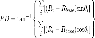(1)

where R_base is the baseline firing rate during the 200 ms prior to stimulus onset and R_i is the response rate to stimulus motion in the direction of θ_i. If the denominator in Eq. 1 was equal to 0, PD was defined either as 90 or 270° depending on the sign of the numerator. We also computed a directional selectivity index for each neuron

(2)

where R_pref and R_null are, respectively, the firing rate for stimulus motion in the preferred and opposite directions and R_base was previously defined. We considered the responses of a neuron to be directional selective if DSI was >0.5.

We computed the Fano factor from responses to stimulus motion at each neuron's preferred speed as the variance of spike count divided by the mean spike count. Data were included for only 162 neurons for which we had accumulated ≥50 responses to the preferred stimulus and which had response latencies <100 ms. The analysis window for the Fano factor began at response onset and varied from 50 to 400 ms. We also analyzed the Fano factor in a 500-ms window that began at stimulus onset, even though this interval included some baseline activity that was present before the onset of the neural response.

Computer simulations of MT population responses

We used a pool of N_ps × N_pd model neurons to simulate MT population responses, where N_ps is the number of preferred speeds of the model neurons, evenly spaced in units of log₂ (speed) from 0.5 to 256°/s. N_pd is the number of the preferred directions, evenly spaced from 0 to 360°. Except where noted, N_ps = 46 and N_pd = 90, creating model populations of 4,140 neurons. In creating model MT population responses, we chose equations and parameter values designed to mimic the mean response of neurons as a function of their preferred speed and direction, the variance of their responses, and the noise correlations between neurons subsequently documented in the results. The result was a noisy model population, where the statistics of the noise simulated the statistics of the actual population response in MT. Nonetheless, the model population was sanitized in the sense that the peak response of all model neurons had the same value. Allowing the peak responses to vary realistically adds several complications and we have chosen to leave this issue for later work.

The mean response of a given MT neuron was modeled as the separable product of two Gaussian functions

(3)

where θ and S indicate the direction and speed of stimulus motion, g indicates the peak response amplitude, PD and PS are the preferred direction and the preferred speed of the neuron, and σ_θ and σ_s are the SDs of the Gaussian tuning curves for direction and speed, respectively. We dealt with the circular nature of direction tuning by making sure that the difference between the direction of target motion and preferred direction was corrected to remain on the range [−π, π]. We chose to use Gaussian speed-tuning curves because they are more easily defined than the spline fits used in our data analysis and provide an excellent description of the speed-tuning curves of most MT neurons (Lisberger and Movshon 1999; Nover et al. 2005). We simulated the responses of the entire model population to 200 presentations of a stimulus moving at a given speed and direction. On each simulated “trial,” the response of each neuron in the population was picked from a normal distribution whose mean was determined by Eq. 3, and whose variance was equal to the response mean.

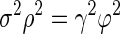
To model neuron–neuron correlations among neurons, we enforced a prescribed covariance on the full population of neuronal responses within each simulated trial (adapted from Shadlen et al. 1996; see their appendix 1: Covariance). The expected correlation coefficient between any pair of neurons i and j is determined by

(4)

where r_max is the expected “maximum correlation coefficient” among all neuron pairs; ΔPD_i,j and ΔPS_i,j are, respectively, the differences between the preferred directions and speeds of the two neurons; τ_d and τ_s are the direction and speed constants that specify the rate of decay of correlations as functions of ΔPD and ΔPS, respectively; and ΔPD_max = 180°, ΔPS_max = 255.5°/s. We set r_i,j to be the separable product of two exponentials based on our observation of neuron–neuron correlations in MT (see results), and we adjusted r_max, τ_d, and τ_s manually to approximate the mean and the structure of noise correlations in MT, as measured in our physiological experiments. The adjustment was performed interactively, graphically viewing the structure of the resulting correlations in the model population in relation to those in our data. The alternative of an automated optimization would have been both conceptually and technically challenging for the large model populations explored in our computation analyses.

Decoding model

We used a vector-averaging computation to decode, concurrently, estimates of stimulus speed and direction from model MT population responses. The vector-averaging computation is described as

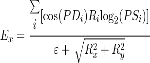(5)

(6)

(7)

(8)

where E_x and E_y are the decoded horizontal and vertical eye velocities (in log₂ unit), respectively; R_i is the simulated response of the ith neuron within the neuron pool; and ɛ is a constant and was set to 0.05. The term ɛ biases the decoding toward small velocities if the amplitude of the population response is low (Churchland and Lisberger 2001; Priebe and Lisberger 2004; Weiss et al. 2002). E_x and E_y are then combined to estimate target speed and direction

(9)

(10)

We computed SPD_est and DIR_est for each of the 200 simulated trials and calculated the means and the variances of the decoded stimulus speeds and directions.

The decoding model described by Eqs. 5–10 performs a vector-averaging computation, but it differs from the conventional vector-averaging model in that it simultaneously decodes stimulus speed and direction. Inspired by the need to eventually transform the sensory representation in retinal coordinates to the pulling coordinates of the extraocular muscles, we constructed the model to evaluate the stimulus speed along the horizontal and vertical axes. The model weights the neural responses with a cosine or sine function for computing horizontal or vertical speed (Eqs. 5 and 6). The weighting functions give the greatest weight to the responses of neurons with preferred directions close to the cardinal axes and also implement an opponent motion computation through the negative halves of the cosine and sine weighting functions. We previously showed that decoding based on an opponent motion signal was needed to account for the effect of apparent motion stimuli on the MT population response and the initiation of pursuit (Churchland and Lisberger 2001).

RESULTS

Our goal was to ask whether the structure of the variation in the neural code in area MT could, in principle, lead to the variation we previously quantified in smooth-pursuit eye movements. After developing a simple model to motivate the potential importance of correlations between neurons, we go through two steps. First, we establish the requisite database by characterizing the structure of neuron–neuron correlations through examining how r_sc depends on the differences between preferred stimuli of a pair of neurons. Unlike prior studies (Bair et al. 2001; Zohary et al. 1994), we pay particular attention to correlations in the first 150 ms of MT responses because this is the part of the response that drives pursuit. Then, to reach our stated goal, we elaborate the computer model sketched in Fig. 1 to decode stimulus direction and speed based on MT population responses that comprise realistic mean responses, neural response variations, and correlations between neurons. The computational analysis allows us to explore the implications of noise correlations in MT for variation in the initiation of smooth-pursuit eye movements (Osborne et al. 2005, 2007).

Computational analysis of the general effect of correlations between neurons on variation in estimates of target speed and direction

The MT population model described in methods creates population responses like those illustrated in Fig. 1. The color map in Fig. 1A1 shows the mean population response across trials for target motion at 16°/s in direction 135° (up and left). Each pixel shows the response of a model neuron with a given combination of preferred directions and speeds. The peak of the population response occurs in neurons with preferred direction and speed equal to target direction and speed. In individual trials, the responses of the individual model neurons are much more variable, as shown by the superimposed population responses for 20 trials, plotted as functions of preferred direction and speed in Fig. 1, A2 and A3, respectively.

If we draw 200 population responses and decode each using the vector-averaging computations described by Eqs. 5–10, we find that the variances of the estimates of target speed and direction depend critically on the amplitude and structure of the noise correlations among MT neurons. For all except the filled orange symbols in Fig. 1, B and C, the correlations were structured to be larger, on average, for pairs of neurons with similar preferred speeds and directions compared with those for pairs of neurons with quite different preferred stimuli. For any given level of structured noise correlation, the variances of the speed and direction estimates decline as a function of the number of neurons in the model population (Fig. 1, B and C). Further, for structured correlations, the variances of the speed and direction estimates increase as a function of the magnitude of the noise correlation in the population (Fig. 1, B and C). As others have pointed out (Medina and Lisberger 2007; Shadlen et al. 1996; Zohary et al. 1994), the variance reduction achieved by increasing pool size becomes quite limited as the magnitude of noise correlations increases.

We can gain an intuition for the effect of noise correlations on readout variance by understanding that structured noise correlations make neighbors in the population response covary more than do nonneighbors. Therefore structured noise correlations have the same effect as a reduction in the number of neurons in the pool. If one is simply averaging across a population of correlated neurons, then the same intuition holds for the effect of noise correlations that lack structure (Shadlen et al. 1996; Zohary et al. 1994); averaging reduces only the noise that is independent across neurons, not the variation that is correlated across neurons.

For a vector average decoding computation, and possibly other decoding computations, the structure of the noise correlations is critical. If noise correlations were independent of the difference in the preferred stimuli of neurons, then increasing the noise correlation would cause the responses of all neurons to fluctuate up and down together. The center of mass of the population, which is what vector averaging estimates, would fluctuate little because of the noise correlations. For example, we simulated an MT population response where the noise correlations averaged 0.3 and were unstructured in the sense that the magnitude of the correlations was independent of the differences between neurons' preferred speeds and directions. The resulting variances of the speed and direction estimates (Fig. 1, B and C, filled orange symbols) were comparable to those obtained when we assumed no correlations among neuronal responses (Fig. 1, B and C, open black symbols). We have no explanation for the fact that the speed variance of the population with large unstructured correlations is lower than that for the population without correlations for populations of <2,000 neurons, but larger for populations of 4,000 neurons. However, repetition of the simulation shows that this tiny effect is repeatable and therefore probably real.

Figure 1 explains how noise correlations can lead to quite variable estimates of stimulus parameters, even when the estimates are obtained by decoding from a large population of noisy neurons. The relatively large variance of the population decoding occurs only when the population contains noise correlations with a structure that emphasizes correlations between neurons with similar stimulus preferences. Our demonstration reiterates the principle established previously by many others (e.g., Abbott and Dayan 1999; Averbeek et al. 2006; Shadlen et al. 1996) that structured noise correlations in a population response have an effect on the estimates obtained through population decoding. The goal of this study is to go further in the context of a specific behavior and to understand quantitatively the potential relationship between noise correlations in MT and the trial-by-trial variation in the direction and speed of pursuit eye movements.

Physiology database and correlation between responses of an exemplar MT neuron pair

We simultaneously recorded from 61 groups of two to five well-isolated neurons in area MT of two rhesus monkeys. Our database included the responses from 181 neurons, giving rise to 165 simultaneously recorded neuron pairs. All neurons included in our database passed the screening requirement that the firing rate in the interval from 50 to 500 ms after motion onset was significantly greater than the baseline activity during the interval 150 ms before stimulus onset, for at least one stimulus condition; few MT neurons failed this criterion. Thirty-nine of the 165 neuron pairs (24%) were recorded from the same electrode and the remaining 126 pairs were recorded from different electrodes separated by 305 to 1,220 μm. Examples of significant correlations were found with all electrode separations. Some of our experimental paradigms were tested only on a subset of the total 165 pairs of neurons.

The responses of MT neurons vary widely from trial to trial even when the same visual motion stimulus is used repeatedly. Between many MT neuron pairs, the response variation is correlated, as illustrated in Fig. 2A for an exemplar MT neuron pair. Each dot represents the responses of these two neurons for different presentations of a given target motion, showing that the spike counts of the two neurons covaried: if the spike count of one neuron was higher or lower than the mean in one trial, then the spike count of the other neuron in the same trial also tended to be higher or lower. The correlation coefficient of the spike count r_sc was 0.64. It was significantly different from zero (P < 0.05) and from the correlation coefficients calculated for trial-shuffled data (t-test, P < 0.05).

FIG. 2. — Absence of effect of exact location of random dots on noise correlations. A: spike count correlation of the responses from an example middle temporal visual area (MT) neuron pair with r = 0.64. Each symbol represents data from a single trial and shows spike counts in z-scores of 2 simultaneously recorded neurons. Visual stimuli comprised presentations of 201 different random-dot textures moving coherently in a fixed direction at 16°/s. B: scatterplot of the correlation coefficients computed from trials that used different vs. the same dot texture on every repetition of the stimulus. Each symbol shows data from one pair of MT neurons and the oblique dashed line has a slope of 1. C and D: averaged cross-correlograms (CCGs) under the random- (C) and fixed-seed (D) conditions for 27 neuron pairs that showed significant spike timing correlation. The y-axes plot the firing rate of one neuron at each time lag conditional on a spike at *time 0* in the other neuron, defined as the number of coincidences in each bin of the CCG divided by the bin width of 1 ms. All responses were calculated during the total 500-ms motion presentation.

Effect of randomizing the dot pattern on neuronal correlation

For a sample of 101 MT neuron pairs, the value of r_sc did not significantly depend on whether the spatial pattern of the dot texture was the same or different across trials (paired t-test, P = 0.24). The absence of an effect of the spatial pattern is documented in Fig. 2B, which plots the values of r_sc when the same dot pattern was used on each stimulus versus the values when the dot pattern was different for each stimulus. The two neurons in each pair of Fig. 2 were recorded from different electrodes, so the spikes of each neuron could be detected even when the two neurons fired within a very short time interval. Twenty-seven of the 101 neuron pairs showed significant spike timing correlation in cross-correlograms, but we did not find any significant differences between the CCG in the random-seed (Fig. 2C) and fixed-seed conditions (Fig. 2D). We conclude that trial-to-trial variation of the details of the random-dot pattern does not significantly change neuronal correlation in MT. Thus even though all the results in the rest of this study were obtained using the dot textures generated with random seeds, we think that the values of r_sc reported in Figs. 3–10 reflect true noise correlations, rather than signal correlations generated by variation in the dot pattern in the visual stimulus. For 14 neuron pairs that provided enough data during fixation in the dark, we also found that the spike count correlations were statistically the same for spontaneous and stimulus-driven activity.

FIG. 3. — Structure of the relationships between spike count correlation *r_sc* and the difference between the *preferred speeds* (PS) (A, D), *preferred directions* (PD) (B, E), and the separation of receptive field (RF) centers (C, F) of the neuron pairs. Each symbol plots the correlation coefficient for one neuron pair. The red symbols represent statistically significant correlations (P < 0.05). A–C: correlation coefficients were based on the initial 150 ms of the neurons' responses to moving stimuli. D–F: correlation coefficients were based on the overall responses during the 500-ms motion presentation period. The gray bands in A and B show the mean ± 1SD of the correlations between pairs. In B and E, “Non-DS” refers to the pairs in which at least one neuron was not directionally selective (DSI <0.5).

FIG. 10. — Contrast dependence of noise correlations. A and B: distributions of the noise correlation coefficients at stimulus contrasts of 5 and 20%. C: the mean correlation coefficient as a function of stimulus contrast. The error bars indicate SEs. Data are from 87 neuron pairs that were studied for stimuli of different contrasts. Horizontal dashed line shows the mean *r_sc* obtained when the stimulus was a high-contrast random-dot patch, averaged across the 43 neuron pairs studied with both patches and square-wave gratings.

Structure of noise correlations in MT

The spike count correlations vary considerably across pairs of MT neurons, with values of r_sc ranging from −0.35 to 0.65 in our sample of pairs. Because we have based our calculations of r_sc on data from a large number of trials (≥289 trials, median = 504) pooled across the responses of neurons to stimulus motion at eight different speeds, we think that the wide variation is a feature of the neural population in MT and not simply a statistical aberration (see controls described in methods).

Some of the variation in r_sc could be attributed to the differences between the response properties of the two neurons in each pair. When the neurons had similar preferred speeds, preferred directions, or receptive field locations, r_sc tended to be positive and to have a larger value (Fig. 3) . The same trends appeared whether r_sc was based on the full 500-ms response of the neurons (Fig. 3, D–F) or the first 150 ms of the responses (Fig. 3, A–C), although the correlations were somewhat smaller when measured on the basis of the first 150 ms of the responses (Table 1). Considering the whole sample of 165 pairs of MT neurons together, the mean value of r_sc was 0.064 versus 0.077 during the first 150 ms of the response versus the full 500 ms of motion. Both values were different from zero with very high statistical significances.

TABLE 1.

Summary of the mean noise correlations in pairs of MT neurons, divided according to whether the two neurons in each pair have more versus less similar preferred directions, preferred speeds, and receptive field (RF) separations

	Preferred Direction		Preferred Speed		RF Separation
	ΔPD < 60°	ΔPD > 60°	ΔPS < 20°/s	ΔPS > 20°/s	ΔRF < 7.5°	ΔRF > 7.5°
Noise correlation, 500 ms	0.14	0.028	0.11	0.0390	0.095	0.025
Statistical significance	P = 6.7 × 10⁻⁷		P = 5.6 × 10⁻⁴		P = 0.0028
Noise correlation, 150 ms	0.12	0.020	0.09	0.0335	0.078	0.024
Statistical significance	P = 6.7 × 10⁻⁷		P = 0.0015		P = 0.006
Number of pairs	69	74	87	78	122	43

Open in a new tab

“Noise correlation” is based on eight speeds of target motion for each pair of cells and then averaged across many pairs. “Statistical significance” is based on a comparison of the two groups of pairs with more versus less similar stimulus preferences.

The effect of the difference in stimulus preferences on r_sc appears in a different form in Fig. 4, where the pairs have been divided into two groups depending on whether the two neurons had more or less similar stimulus preferences. Pairs showed larger noise correlations when their preferred speeds differed by <20°/s, their preferred directions differed by <60°, or their RF centers were separated by <7.5°. In each panel of Fig. 4, the correlations of pairs with more similar (black) versus less similar (gray) stimulus preferences were significantly different (Table 1). The magnitude and statistical significance of the differences did not change materially in the face of even fairly large changes in the exact values used to divide the pairs into two groups based on differences in preferred speed, preferred direction, or receptive field separation. Moreover, plotting r_sc as a function of the ratio of the preferred speeds (rather than their difference) did not alter the structure of r_sc in relation to the difference in the preferred speeds of the two neurons in a pair.

Differences in preferred stimulus parameters appear to operate collectively in determining the degree of noise correlation between two MT neurons. The three-dimensional graph in Fig. 5 plots r_sc in relation to ΔPD and ΔPS between the pairs of MT neurons. It shows that r_sc was strongest for the neuron pairs having similar preferred directions and preferred speeds (bottom left). The value of r_sc decreased as the difference between the preferred directions or preferred speeds increased, moving up and to the right or down and to the right on the graph. To test for separable effects of ΔPD and ΔPS in determining the magnitude of noise correlation, as assumed in Eq. 4, we evaluated the effect of ΔPD for neuron pairs with large versus small values of ΔPS (and vice versa). The results were consistent with the assumptions of Eq. 4, but many more neuron pairs would have been needed to make a statistical statement. Finally, by plotting r_sc in relation to ΔPS and the distance between the centers of the neurons' receptive fields, we noted that correlations were not necessarily high between pairs whose receptive fields were close to each other; strong r_sc appeared only when neuron pairs also shared similar preferred speeds (data not shown).

FIG. 5. — Three-dimensional plots of spike count correlation *r_sc* in relation to the differences in PS and PD between the 2 neurons in each pair. Filled circles show pairs with significant positive correlations. Correlation coefficients were based on the overall responses to 500 ms of motion. The graph shows data for 143 pairs of directional-selective MT neurons.

Time course of noise correlation in MT

The responses of MT neurons change over time following stimulus motion onset, typically showing an early transient and a late sustained response (Lisberger and Movshon 1999; Osborne et al. 2004; Priebe et al. 2002; Schlack et al. 2007). To understand the possible relationship between the temporal dynamics of visual motion processing and noise correlations, we next characterized the time course of neuronal correlation in MT. For each pair of MT neurons, we computed the spike count within 100-ms windows positioned at 10-ms increments through the response period and computed r_sc for all pairs of 100-ms windows. This yielded correlation maps like those shown in Fig. 6, which were averaged across neuron pairs to reveal the main temporal features of r_sc. The average correlation map for all 165 pairs of MT neurons in our sample (Fig. 6A) shows the strongest correlation along the diagonal, indicating responses occurring at the same time in the two neurons. The correlations were slightly stronger at the onset of the response (Fig. 6A, bottom left) than later in the response. Correlations off the main diagonal were small, indicating weak temporal correlations across neurons (referred to later as cross-temporal correlation).

FIG. 6. — Correlation maps as a function of time during the response to stimulus motion. The color of each pixel shows the mean correlation coefficient as a function of the times within the response of the 2 neurons. A: averages across all 165 neuron pairs. B and C: pairs with significant positive (n = 72) or negative (n = 18) correlations. All 3 correlation maps use the same color bar. Correlation coefficients were based on a series of 100-ms analysis windows incremented in 10-ms steps through the response. D: correlation along the diagonal of the 3 correlation maps plotted as a function of time from the onset of the neural response. *Black*, *red*, and *blue traces* show correlations for all neurons and neurons with significant positive or negative correlations. Time t in the plots indicates the time from t to t + 100 ms and t = 0 signifies the start of the neural response. The axes run to 250 ms, representing data from 0 to 350 ms after the onset of the response. Because some neurons had response latencies as long as 150 ms, 350 ms of data comprise the entire response for some neurons.

To better understand the detailed temporal properties of noise correlations in MT, we next averaged the correlation maps separately for the pairs of MT neurons that showed only significant positive (Fig. 6B, n = 72) or negative correlations (Fig. 6C, n = 18). Again, the correlations were strongest along the diagonal and slightly stronger early versus late in the response. Although not visible in Fig. 6 because of our choice to display all three graphs using the same color map, the strongest negative correlation occurred about 20–40 ms later than the strongest positive correlation. The nearly flat time course of the correlations with a slight early inflection is emphasized by Fig. 6D, which plots the correlations along the main diagonal as a function of time from the onset of the neural response.

Time interval of neural response and noise correlation

Table 1 shows that the mean MT noise correlations computed from the first 150 ms of the response to stimulus motion were smaller than those based on longer, 500-ms responses to motion. A scatterplot of the correlation coefficients computed using these two time intervals (Fig. 7A ) confirms the effect of analysis interval. For positive correlations, r_sc tends to be larger based on the overall responses than when based on the initial 150-ms responses; for negative correlations, r_sc tends to be more negative when based on the overall responses than when based on the initial responses. Linear regression of the data in Fig. 7A revealed a slope of 0.75 that was statistically smaller than 1.0 (95% confidence interval: 0.68–0.81). We obtained exactly the same relationship when we avoided potential artifacts caused by low spike counts during the shorter time interval by restricting our analysis to 70 pairs that emitted enough spikes so that the distributions of spike counts were Gaussian for both neurons. The slope of the relationship between r_sc in the first 150 ms of the neural response versus r_sc in the full 500 ms of the response was 0.745 and was statistically indistinguishable from the value of 0.75 found with the full set of neuron pairs. This control analysis implies that the effect of analysis interval on r_sc cannot be explained by lower spike counts during the shorter time interval. To systematically study the effect of the duration of the analysis interval on r_sc, we calculated the averaged r_sc of the 165 neuron pairs using various time intervals. The intervals always started from response onset and had durations of 100 to 400 ms in 50-ms steps. Once the analysis interval exceeded 200 ms, the average value of r_sc increased steadily as the duration of the analysis interval increased (Fig. 7B).

FIG. 7. — Analysis of the growth of noise correlation as a function of the duration of the analysis window. A: scatterplot comparing correlation coefficients based on the responses during the initial 150 ms of the neural response vs. the full 500 ms of the stimulus. The solid line has a slope of 1 and the dashed line shows the regression fit with a slope of 0.75. B: the averaged correlation coefficient across 165 MT neuron pairs as a function of the duration of the analysis window. C: average Fano factor of spike count as a function of the duration of the analysis windows. In B and C, the point at an analysis interval of 500 ms shows results for analysis of the entire 500-ms duration of the motion stimulus, starting from the onset of the stimulus motion. All other intervals started from the time of response onset. Error bars indicate SEs.

The increasing relationship between r_sc and the duration of the analysis interval can be understood in terms of the prior finding of temporal correlations in the spike counts of individual MT neurons (Osborne et al. 2004). We make this statement analytically rigorous by considering a response interval T with two equal subintervals T₁ and T₂ and two neurons with responses a_i and b_i during the ith interval, where i = [1, 2]. Then the definition of cross-correlation yields

(11)

Math contained in the appendix derives a relationship that describes the conditions under which r_sc does not change as the duration of the analysis interval grows

(12)

where σ² is the response variance during each time epoch; ϕ² is the covariance between the responses of two neurons during the same time epoch; ρ² is the covariance between the responses of two neurons during different time epochs (reflecting cross-temporal correlation); and γ² is the covariance between the responses of the same neuron during different time epochs (reflecting autotemporal correlation). If the left side of Eq. 12 is larger (or smaller) than the right side, then r_sc will increase (or decrease) as the duration of the analysis interval increases. When r_sc is stable in the face of changes in analysis interval

(13)

Our data were consistent with the analytical predictions of Eqs. 12 and 13, both for the full sample of neuron pairs and for the smaller sample where we were able to avoid potential artifacts due to small spike counts. Analysis of our 165 pairs of MT neurons for T = 400 ms and T₁ = T₂ = 200 ms revealed positive auto- and cross-temporal correlations (Table 2), indicating that the assumptions made in the appendix are consistent with our data. Evaluating Eq. 12 with the results obtained by analysis of our data (Table 2) reveals that σ²ρ² = 0.0215 and ϕ²γ² = 0.0088. Because σ²ρ² is greater than γ²ϕ², r_sc for the analysis interval of duration T = 400 ms should be greater than r_sc for the analysis interval of duration T₁ = 200 ms: the noise correlation r_sc should and does increase as a function of analysis time interval.

TABLE 2.

Auto- and cross-covariances across time in our sample of 165 pairs of MT neurons

	Time Interval T₁		Time Interval T₂
Neuron a	σ²	––γ² = 0.15––	σ²
	\|		\|
	\|	ρ²:	\|
	\| ϕ² = 0.063	cov (a₁, b₂) = 0.021	\| ϕ² = 0.062
	\|	cov (b₁, a₂) = 0.022	\|
	<\|		\|
Neuron b	σ²	––γ² = 0.13––	σ²

Open in a new tab

As described in the text, σ² is the response variance during each time epoch; ϕ² is the covariance between the responses of two neurons during the same time epoch; ρ² is the covariance between the responses of two neurons during different tome epochs (reflecting cross-temporal correlation); and γ² is the covariance between the responses of the same neuron during different time epochs (reflecting autotemporal correlation). Numbers were obtained by analysis of our sample of MT neuron pairs during T₁ = T₂ = 200-ms time intervals.

Algebra at the end of the appendix shows that positive temporal correlations should cause the Fano factor to increase as a function of analysis interval. Figure 7C confirms this prediction, in agreement with a previous study that recorded from single neurons in area MT of anesthetized monkeys (Osborne et al. 2004). We note that the consistent relationship between Fano factor and the duration of the analysis window is at odds with the traditional view of cortical neurons as “Poisson” encoders, with spike count variance equal to spike count mean. In evaluating this deviation from traditional thought, we need to remember that the Fano factor is measured across trials and reflects the combination of trial-by-trial variations in the underlying firing rate and the stochastic nature of spike generation. Our data cannot separate these effects: the increase in Fano factor across a trial could be caused by an increase in the variance of either the underlying firing rate or the spike generation.

Speed dependence of noise correlations in MT

To gain a better understanding of the origin and meaning of correlations in MT, we next examined how r_sc changed with stimulus speed, using only neuron pairs that had similar direction and speed preferences (ΔPD <90° and ΔPS <25°/s) and whose RF centers were separated by <10°. We analyzed only neuron pairs that were tested with ≥50 repeated stimulus presentations at each of the eight stimulus speeds (70 MT pairs).

Figure 8 shows how r_sc varies with target speed. The scatterplots (Fig. 8A) give a sense of the data on which the correlation analysis is based for one neuron pair, by showing the covariation of the z-scored trial-by-trial neuronal responses for each of eight stimulus speeds, ranging from 1 to 128°/s from left to right. For the three pairs of neurons summarized by the graphs in Fig. 8, B–D, the strongest correlation occurred at the rising flanks of the speed-tuning curves for the pair of neurons and lower correlations were present at the peaks and on the declining flanks of their tuning curves.

We assessed the speed dependence of the correlation for each pair of MT neurons in relation to the geometric mean of the two neurons' speed-tuning curves, termed the “joint speed-tuning curve.” Across our population of 70 neuron pairs the averaged joint speed tuning had a peak at the “joint preferred speed” of 16°/s (Fig. 9A) . For the same population, the average value of r_sc was larger at lower speeds than that at higher speeds (Fig. 9B). Mean r_sc at 1, 2, 4, and 8°/s ranged from 0.149 to 0.173, whereas r_sc at 16, 32, 64, and 128°/s ranged from 0.099 to 0.126. The mean r_sc at the population averaged joint preferred speed of 16°/s was significantly smaller than the mean r_sc of 0.173 at 8°/s (one-tailed paired t-test, P = 0.00085) and the mean r_sc of 0.154 at 4°/s (one-tailed paired t-test, P = 0.014). Note that these values of r_sc are higher than those in the overall sample of pairs because these pairs were selected to have similar stimulus preferences and therefore higher values of r_sc.

FIG. 9. — Speed dependence of noise correlation summarized for 70 neuron pairs with similar stimulus preferences. A: averaged joint speed-tuning curve across pairs. B: averaged correlation coefficients across pairs as a function of stimulus speed. Error bars in A and B indicate SEs. C: summary of the relationship between the speed of the largest value of *r_sc* and the joint preferred speed. Each symbol is sized to indicate the number of pairs that plotted at each site in the graph. The 4 symbol sizes indicate that 1, 2, 3, or 5 pairs corresponded to each location in the graph. Data are for 50 neuron pairs that showed significantly positive correlation at one or more stimulus speeds. C1: marginal distribution of the speed of the largest *r_sc*. C2: marginal distribution of the joint preferred speed.

To determine whether the relationship between the properties of the tuning curves and the value of r_sc held on a pair-by-pair basis, we calculated the speed at which r_sc reached its peak and compared this “speed of the largest r_sc” with the joint preferred speed for each pair. Because it made sense to explore the relationship between maximum r_sc and speed tuning only when the correlation was significant, we limited our pair-by-pair analyses to the 50 neuron pairs that were part of our sample for assessing the effect of target speed, and that showed significantly positive correlation at one or more stimulus speeds.

Figure 9C shows that the speed of the largest r_sc generally was lower than the joint preferred speed, indicating that the noise correlations were consistently higher on the rising slope of the joint speed-tuning curve. Here, the diameter of each symbol is proportional to the number of pairs that had the x and y values associated with that location on the graph. The majority of the pairs (35/50 pairs) had speeds of the largest r_sc lower than their joint preferred speed (those circles below the unity line of Fig. 9C) and 9 of the remaining 15 pairs had speeds of the largest r_sc equal to their joint preferred speed. One possibility is that r_sc simply is larger at lower speeds. However, two factors make it worth considering the alternative that the speed of the largest r_sc is related to the joint preferred speed of the pair of neurons. First, Fig. 9C gives the impression that the unity line is a better cutoff than would be any horizontal line, with many pairs plotting just below the unity line and very few above it. The median speed of the largest r_sc is 4°/s, significantly smaller than the median joint preferred speed of 16°/s (one-tailed signed-rank test, P = 5.8 × 10⁻⁵). Second, statistical analysis showed that r_sc drops significantly at the joint preferred speed compared with the maximum r_sc occurring at the rising flank of the composite speed-tuning curve. For the 35 neuron pairs whose speed of the largest r_sc was smaller than the joint preferred speed, the median r_sc at the speed of the largest r_sc was 0.42 and was significantly larger than the median r_sc of 0.19 at the joint preferred speed (unpaired signed-rank test, P = 8.4 × 10⁻⁵). The two alternatives might be distinguished by future experiments on pairs of neurons with low values of preferred speed.

Contrast dependence of noise correlations in MT

Measurements in 87 MT neuron pairs using square-wave gratings revealed a consistent increase in r_sc as stimulus contrast was lowered. For example, comparison of the distribution of noise correlations for stimulus contrast of 5 and 20% (Fig. 10, A vs. B ) reveals a clear difference. The mean correlation coefficient across the 87 neuron pairs at 5% contrast was 0.15, significantly greater than the mean correlation coefficient of 0.09 at 20% (one-tailed paired t-test, P = 0.017). Analysis across a wider range of contrasts revealed that the effect of contrast was strongest when contrast was low. In population averages (Fig. 10C), correlation coefficients were strongly reduced as the stimulus contrast increased from 5 to 20%, but then increased slightly as contrast increased further to 80%. The same population of neurons had a mean r_sc of 0.094 when the stimulus was a high-contrast patch of random dots (horizontal dashed line in Fig. 10C). The effect of stimulus contrast on noise correlations is potentially important because, as illustrated in Fig. 1, an increase in magnitude of structured noise correlations also predicts an increase in the variance of any behavior decoded from the MT population response. Our lab is currently testing the effects of contrast on the trial-by-trial variation in the initiation of pursuit.

Decoding stimulus speed and direction from MT population responses

We already know (from Fig. 1) that structured noise correlations lead to a failure of noise reduction in decoding large model populations. Therefore our goal in this section was to use the same population model and decoding computations, but to fix the noise correlations of model population responses to match our data and then explore the conditions under which realistic model population response could be the source of variation in pursuit direction and speed of the scale reported in our prior publications (Osborne et al. 2005, 2007).

We created model MT population responses with parameters chosen to match the data from our recordings. To match the degree of variation across the model neurons to that in MT for an analysis interval of 150 ms, we drew neuronal responses from distributions that had variance equal to the mean response. Figure 1, A2 and A3 illustrates the variation across the model population on individual trials. To match the correlation structure characterized in our physiology experiments, we adjusted r_max, τ_s, and τ_d in Eq. 4 interactively, evaluating the structure of r_sc of the model population compared with our data from MT. The effects of the parameters interacted to some degree, requiring multiple iterations. To a first approximation, however, r_max controlled the magnitude of noise correlations for pairs with similar preferred speeds and directions, whereas τ_s and τ_d controlled the correlations for pairs that differed substantially in preferred speed and direction, respectively. With a few iterations, it was possible to achieve the good agreement between the model and experimental populations illustrated in Fig. 11. Here, we have plotted r_sc of the model neurons as functions of their stimulus preferences, with r_max, τ_s, and τ_d set to 0.36, 0.3, and 0.4, respectively. The mean r_sc across all 1,035 model neuron pairs in Fig. 11A was 0.072; r_sc averaged 0.11 and 0.046 for pairs whose preferred speeds differed by less than or more than 20°/s. The mean r_sc across all 4,005 neuron pairs in Fig. 11B was 0.079; r_sc averaged 0.11 and 0.066 in pairs whose preferred directions differed by less than or more than 60°. The gray ribbons in each panel, also shown in Fig. 3, A and B, summarize the mean ± 1SD of the actual correlations in our sample of MT pairs. They document reasonably good agreement between the correlation structures in our model populations and in MT. We did not vary the correlation structure as we explored our model.

FIG. 11. — Structure of spike count correlations for neuron pairs in a typical model MT population response. The parameters used in the model were: r_max = 0.36, and τ_s = 0.3, and τ_d = 0.4. A: relationship between *r_sc* and the difference between the preferred speeds of model neuron pairs whose preferred directions were equal to stimulus direction. The mean *r_sc* across all 1,035 pairs of model neurons was 0.072. B: relationship between *r_sc* and the difference between the preferred directions of 4,005 model neuron pairs whose preferred speeds were equal to stimulus speed. The mean *r_sc* across all 4,005 pairs of model neurons was 0.079. The gray ribbons are replotted from Fig. 3 and show the mean ± 1SD of the noise correlations in our sample of pairs of MT neurons.

Our model population had three free parameters: response gain, speed-tuning width, and direction-tuning width (Eq. 3). Of these, response gain was treated as unconstrained and its meaning will be taken up in the discussion. We adjusted the tuning widths on the premise that it might be possible for the decoding computation to select outputs from only a subset of the full population of MT neurons, perhaps from those with the widest or the narrowest direction tuning. A biologically plausible range is defined by our sample of MT neurons, where the SD of speed tuning σ_s ranged from 0.64 to 2.8 and averaged 1.64 (also see Nover et al. 2005); direction-tuning width, defined as the full width at half-height, ranged from 61 to 177° and averaged 102°. To explore how different sets of parameters might affect the variation in speed and direction of pursuit eye movements, we created 200 model population responses for each of a wide range of possible values for the free parameters. We then used Eqs. 5–10 to decode the 200 population responses and evaluate the mean and variance of the estimates of target speed and direction. Except where noted, the mean estimates of speed and direction were quite accurate, closely reproducing stimulus speed (Fig. 12D) and direction. Note that we systematically varied the parameters across runs of the model, but we set up each run so that every model neuron had the same gain and tuning widths. We recognize that this is not the case in MT and that the variety of parameters among neurons probably influences the predictions of different decoding computations. We see this as a complicated second-level issue that we do not need to confront now to achieve our goal of determining whether the variation in the direction and speed of pursuit could plausibly result from the correlated variation in the responses of MT neurons. Note, again, that the model used in Fig. 12 is the same as the one used in Fig. 1, except that we now have constrained the structure of noise correlations to match the data presented earlier.

The predictions of the decoding model depend strongly and reliably on the parameters of the units in the model population and we can intuitively understand many of the effects in Fig. 12 in terms of the properties of the model population. In general, the variances of the speed and direction estimates decrease as their own tunings sharpen because sharper tuning leads to better power in discriminating small differences (see Zhang and Sejnowski 1999). Figure 12 illustrates four key features of the decoding computations.

First, the variances of both the direction and speed estimates decrease as the units' response amplitudes increase (Fig. 12A). The variances in Figs. 12 and 13 are mostly higher than those in Fig. 1 because we have used lower values for response amplitude in this part of the study.

FIG. 13. — Speed and direction variances of decoded estimates of target speed and direction match the variances of eye speed and direction during open-loop pursuit. A and B: speed variance plotted as a function of the SD of speed tuning in the model MT population. C and D: direction variance plotted as a function of the SD of speed tuning. The 2 columns summarize the performance of models chosen to reproduce different sets of data. Filled and open symbols in the *left column* (A, C) show 2 models designed to match the average performance of monkey subjects from Osborne et al. (2007). The horizontal lines indicate the average variances of those subjects and the vertical dashed lines are plotted at values of the SD of speed tuning that allow the models to reproduce the average variances. The *right column* (B, D) shows models designed to match the performance of 2 monkeys that represent extremes of data obtained in our laboratory. The horizontal dotted and solid lines indicate the variances obtained from monkey Pk, who showed very reliable pursuit initiation, and monkey Mo, who showed the most variable pursuit initiation among recent subjects in our laboratory. Open and filled symbols show models that could reproduce the variances of monkeys Mo and Pk, respectively. The vertical dashed lines indicate the values of the SD of speed tuning that allowed the models to succeed. Parameters of the successful population models are given in the text.

Second, as the direction-tuning width increases, the direction variance increases monotonically (Fig. 12E). However, the speed variance displays a U-shaped function that decreases initially and then increases at direction-tuning widths >140° (Fig. 12B). Analysis of decoding computations with and without an opponent stage implies that the rising phase of the “U” occurs because widening the direction-tuning curve causes some excited neurons to fall on the negative phase of the opponent computation.

Third, as the speed-tuning width increases, the direction variance decreases monotonically (Fig. 12F), whereas the speed variance initially increases and then decreases (Fig. 12C). Exploration of the model showed that the decreasing arm of the speed-variance curve occurs because of edge effects when the speed-tuning width becomes large enough so that the population response does not drop to zero for model neurons with the highest and lowest preferred speeds. The mean speed estimate replicates the stimulus speed within a range of speed-tuning widths, but starts to drop at broad speed-tuning widths (σ_s >2 log units, Fig. 12D).

Finally, the families of curves in Fig. 12, B, C, E, and F indicate that the effects of altering speed and direction tuning bandwidth are largely separable. The amplitudes of the curves for changes in one form of tuning width are simply scaled for changes in the other form of tuning width and the shapes of the curves remain invariant in each graph.

To determine whether the variance of the decoded population responses depended on the population responses themselves or on the structure of the decoding computation, we used two additional decoding computations to evaluate the same population responses. One decoding computation was traditional vector averaging, using separate equations for decoding speed and direction as described for speed by Churchland and Lisberger (2001). The other decoding computation used the same maximum-likelihood calculations described by Jazayeri and Movshon (2006). Both yielded results very similar to those outlined in Figs. 12 and 1, B and C. The effects of varying the parameters were qualitatively the same and quantitatively within 10% of the predictions reported in Fig. 12. The only exception, mentioned earlier, was that the absence of an opponent stage yielded a monotonically decreasing relationship between speed variance and direction bandwidth for maximum likelihood and separate vector-averaging computations. We conclude that the direction and speed variances outlined in Fig. 12, and their parametric dependence, reflect properties of the model population responses we contrived to match the actual population responses in MT.

Population responses that capture the variation of pursuit eye movements in specific subjects

We now show that the variation of pursuit eye movements (Osborne et al. 2007) could emerge based on decoding realistic MT population responses that include realistic noise correlations between pairs of neurons. First, we reproduce the mean variances of eye speed and eye direction during pursuit initiation across monkey subjects from Osborne et al. (2007). Converting the discrimination thresholds (equivalent to 69% correct in a two-alternative forced-choice paradigm) into variance yields values for eye speed and direction, respectively, of 4.1 deg²/s² and 6.0 deg². These values are shown as the horizontal fine lines in Fig. 13, A and C, which also plot the speed and direction variance as a function of the SD of the speed-tuning functions of the model neurons. The vertical dashed lines connecting the two graphs illustrate two different model MT population responses that can predict the variances of direction and speed. For one model population, the response gain, direction-tuning bandwidth, and speed-tuning SD were equal to 6.0, 60°, and 1.7 (in log₂ units); for the other model population, the response gain, direction-tuning bandwidth, and speed-tuning SD were equal to 4.5, 46°, and 1.1. Decoding based on many other intermediate model populations also could reproduce the same pair of speed and direction variances.

Finally, we show that decoding population responses based on different parameters can reproduce a wide range of behaviors. The horizontal dotted and solid lines in Fig. 13, B and D indicate the variances of eye speed and direction based on the discrimination thresholds of two monkeys with widely disparate behavioral variances (J. Yang and S. G. Lisberger, unpublished data). Monkey Pk had small speed and direction variances: 2.3 deg²/s² and 17.2 deg², respectively. The variances of the model readouts matched monkey Pk's pursuit behavior when the response gain, direction-tuning bandwidth, and speed-tuning SD were set to 6.0, 98°, and 1.9, respectively (solid circles in Fig. 13, B and D). Monkey Mo had the most variable pursuit behavior ever quantified in our laboratory, with speed and direction variances of 19.0 deg²/s² and 76.0 deg². The variances of the model readouts matched monkey Mo's pursuit behavior when the response gain, direction-tuning bandwidth, and speed-tuning SD of the model population were set to 2.3, 96°, and 1.3, respectively (open circles in Fig. 13, B and D). We will argue in the discussion that the model parameters used to generate Fig. 13 are physiologically plausible.

DISCUSSION

Our overall goal is to understand how visual motion signals are transformed to drive smooth-pursuit eye movements. One component of that goal is to understand which of the features of pursuit can be attributed to features of the representation of visual motion and which arise downstream in the motor system. For example, our laboratory has hypothesized on the basis of behavioral data that the trial-by-trial variation in the visually driven initiation of pursuit arises from noise in sensory processing (Osborne et al. 2005, 2007) and we have provided evidence from neural recordings that the variation in pursuit arises before the cerebellum (Medina and Lisberger 2007). However, the sensory noise hypothesis raises an obvious and fundamental question: given the large number of neurons that are active in MT for any one stimulus, how can the brain fail to reduce sensory noise to negligible levels by averaging?

Prior analyses have demonstrated that a critical feature of the MT population response—correlations between neurons—could limit the noise reduction available by averaging and that the impact of correlations depends on how the population response is decoded. Herein, we have addressed these issues for the specific case of the relationship between the representation of visual motion in MT and the eye movements emitted at the initiation of pursuit. Even though prior theoretical analyses have treated many aspects of the same issues, we argue that there is merit in addressing the same issues within the context of a behavioral response that can be treated quantitatively. We have done so in two steps. First, we characterized the structure and amplitude of noise correlations in area MT over the behaviorally relevant interval for the initiation of pursuit, an advance relative to prior studies of correlations in longer intervals. Then, we used a computer model to create model neural population responses with realistic correlations, to decode the population response to obtain estimates of target direction and speed, and to evaluate the relationship between the variance of those estimates and the variance of pursuit eye movements.

Properties of noise correlation

We found that noise correlations between pairs of MT neurons were stronger when the neuron pairs had similar speed preferences, similar direction preferences, or small separations between their receptive field locations. Our results extend previous findings in the direction domain for pairs of nearby neurons in MT (Bair et al. 2001; Zohary et al. 1994) and agree with data in the orientation domain for neurons in the primary visual cortex (V1) (Smith and Kohn 2008; Ts'o et al. 1986). Responses of neighboring neurons in inferior temporal cortex (IT) are also correlated (Gawne and Richmond 1993). Our results, together with these previous findings, suggest a common feature of neuronal correlation: noise correlations tend to be stronger between neurons having similar stimulus preferences than between those having different stimulus preferences. It is important that the structure of noise correlation is best described as a trend. For any given location on the x-axis of the graphs in Fig. 3, there is a wide range of noise correlations ranging from negative to positive, even when the average is positive.

One critical advance in our data is that the structure of correlations in MT is the same for the first 150 ms of the neuronal response as that for longer response epochs, although the shorter time interval yields lower values of noise correlation. A recent study in V1 also found that correlation coefficient computed during a 100-ms time interval is smaller than that computed during a 1.28-s interval (Smith and Kohn 2008). Shorter response epochs are important for our overall goal because the visual input for pursuit is a brief pulse of motion of duration ≤150 ms. Importantly, we also were able to understand the relationship between correlation magnitude and the duration of the response epoch in terms of the temporal correlations among and across neurons, which we called auto- and cross-temporal correlations. The existence of autotemporal correlations was known previously (Osborne et al. 2004; Teich et al. 1996). We emphasize that their existence necessitates characterization of correlations within the time interval that is most relevant to the computation required to generate behavior.

Implications of noise correlations for the coding of visual motion in MT

The structure and stimulus dependencies of noise correlations provide some insight into the neural circuit mechanisms that generate the code for motion. Neurons having similar stimulus preferences are more likely to share common feedforward inputs (Alonso et al. 2001; Hubel and Wiesel 1962; Michalski et al. 1983) and to be part of a local network with recurrent connections (Bosking et al. 1997; Douglas and Martin 1991; Gilbert and Wiesel 1983; Somers et al. 1995; Ts'o et al. 1986), compared with neurons having widely different stimulus preferences. This architecture of neural circuitry could contribute to both the correlation between the mean responses representing stimulus features (“signal”) and the correlation of trial-by-trial response variation (noise). Thus the structure of noise correlation follows, to some extent, the strength of signal correlation. The finding that noise correlations are higher for stimuli of lower speed implies that the mechanisms shaping the rising flank of the speed-tuning curve may be different from those shaping the peak and the descending flank of the speed-tuning curve. Finally, our finding that r_sc in MT is higher at low stimulus contrast than that at high contrast may reflect larger spatial pooling and less surround inhibition at low versus high contrast.

Our data on the contrast dependence of correlations are consistent with a similar trend for the spike timing correlation in MT (de Oliveira et al. 1997). Similarly, Kohn and Smith (2005) demonstrated that correlation in V1 is temporally more precise but weaker at high contrast. Note that the speed and contrast dependencies of r_sc cannot be explained entirely by the possibility that correlation increases with firing rate (de la Rocha et al. 2007) because the peak values of r_sc occurred for stimuli that drove submaximal responses.

Implications of correlations for decoding motion signals from MT population responses

The impacts of noise correlation, tuning curve width, and decoding computation on population decoding have been previously treated in a number of studies (Abbott and Dayan 1999; Lee et al. 1998; Oram et al. 1998; Reike et al. 1996; Series et al. 2004; Shadlen et al. 1996; Shamir and Somploinsky 2004; Snippe and Koenderink 1992; Zhang and Sejnowski 1999; Zohary et al. 1994; for reviews see Averbeck et al. 2006; Shadlen and Newsome 1994). Our goal was to consider the same issues in a specific context of realistic model population responses based on extensive recordings from MT, in an effort to predict specific features of the initiation of smooth-pursuit eye movements.

When we decoded a realistic model MT population response, we were able to predict the variances of pursuit speed and direction. By minor variations in the parameters of the model population, we were able to reproduce a fairly wide range of behaviors found in different experimental subjects. Our finding that noise reduction is limited by structured correlations, even with a very large neuron pool, is consistent with the findings by Gawne and Richmond (1993) and Zohary et al. (1994). Compared with independent noise, correlated noise is more likely to propagate through different stages of neural processing and to contribute to the variation of pursuit eye movements.

The exact values of the speed and direction variances depended critically on the parameters of the model population response. Tuning curve bandwidth was an important parameter in principle. The model populations that predicted the averaged variance of pursuit across monkey subjects well had direction tuning bandwidths near the small end of the range and speed-tuning bandwidths were in the middle of the range in our physiological sample. The model populations that predicted the variances of pursuit of two individual monkey subjects had both direction and speed-tuning widths in the middle of the ranges in our physiological sample. These findings suggest that pursuit could be driven selectively by MT neurons with limited direction tuning bandwidths and that the relevant neurons could differ across subjects and might even be adjustable by training. Our computational analysis was constrained by the neuron–neuron correlation structure from our recordings, which were made during fixation of stationary targets. If the correlations were increased somewhat or the structure tightened during the initiation of pursuit, as they are in a direction-discrimination task (Cohen and Newsome 2008), then we might need to choose somewhat different parameters in the model population to reproduce the pursuit variance of different subjects. However, only small changes would be needed.

Response magnitude was also a critical parameter in determining the variances of decoded estimates of speed and direction: smaller-amplitude population responses lead to larger variances. Because we do not know the exact neural code used to decode the population response in MT, we choose to think about the code in terms of spike counts. The mean spike count of the neuronal responses in our data sample during the first 150-ms response was 11.5 spikes. To match the variation of pursuit, the response amplitude in our model ranged from 2.3 to 6.0 spikes. One interpretation of this discrepancy is that the initiation of pursuit may rely on spike counts from a time window <150 ms and that the duration of the time window may vary in different monkey subjects and, again, may be adjustable by training.

The exact decoding computation did not make a large difference in the variance of the estimates of speed and direction, as long as the computation extracted approximately the center-of-mass of the population response. Our figures show detailed results for a variant of vector averaging that converted the population response into commands for the speed of horizontal and vertical eye motion. However, we obtained essentially the same predictions when we used the maximum-likelihood computation of Jazayeri and Movshon (2006) or more standard vector-averaging equations to independently decode target speed and direction. The effects of varying the parameters were qualitatively the same and quantitatively within 10% of the predictions reported in Fig. 12. The only exception, mentioned in results, was that the absence of an opponent stage yielded a monotonically decreasing relationship between speed variance and direction bandwidth for maximum-likelihood and separate vector-averaging computations. We take the similar performance of different decoding computations as evidence that the key factor in determining response variance is the model population response itself.

We prefer the variant of vector averaging described by Eqs. 5–10 as a decoding computation and used it here, for two reasons. First, it solves the problem of converting the retinal representation of visual motion in MT into muscle coordinates. This choice is consistent with the fact that the Purkinje cells in the floccular complex of the cerebellum are primarily tuned to eye movements in cardinal axes. Second, it contains the opponent motion feature that was needed to account for the relationship between MT population responses and an illusion of increased target speed for apparent motion stimuli (Churchland and Lisberger 2001). Note, however, that the opponent motion computation did not have a major impact on the performance of the model in this study, except at high direction tuning bandwidths, because the spontaneous firing rate was zero in our model neurons.

Sensory noise, population decoding, and behavioral variation

In our previous work, we showed that the variation in the initiation of pursuit was low dimensional and could be described in terms of errors in estimating the direction, speed, and time of target motion (Osborne et al. 2005). We also showed that pursuit could estimate the parameters of target motion as well as could perception, implying a common source for the variation in the sensory system (Osborne et al. 2007). For visual motion, extrastriate area MT is a logical place to look for the source of the variation. We have now shown that the structure and magnitude of the correlations between MT neurons and the trial-by-trial variation in neural responses have the correct scale to constitute the source of pursuit variation. Further, the agreement between the magnitudes of pursuit and perceptual variation means that area MT could also be the source of the perceptual variation (Osborne et al. 2007).

Our recordings from the floccular complex of the cerebellum (Medina and Lisberger 2007) show that little or no noise is added to the initiation of pursuit downstream from the cerebellum, assigning the origin of pursuit variation to upstream structures. Still, it remains possible that a better prediction of behavioral variation would come from assuming that some variation arises from MT, whereas the rest comes from downstream noise. At one extreme, the decoding mechanisms for pursuit actually may be able to eliminate most or all the noise in the responses of MT neurons and that pursuit variation originates between MT and the cerebellum. Decoding computations could minimize the variation in their estimates of target motion either by ignoring correlations (e.g., Series et al. 2004) or by selecting from populations of MT neurons that would minimize the variation in the decoded output. The possibility that some pursuit variation is added downstream from MT seems particularly apt in individuals whose pursuit variance is higher than would be predicted by measurements of perceptual discrimination thresholds in highly trained humans and monkeys (de Bruyn and Orban 1988; Liu and Newsome 2005), even though we can reproduce the larger values of pursuit variance by careful selection of the parameters used to generate model MT populations. We cannot exclude the possibility that some behavioral variation arises after the sensory representation in MT, but the present study supports the plausibility of our prior suggestion of a common sensory source for pursuit and perceptual variation (Medina and Lisberger 2007; Osborne et al. 2005, 2007), without the addition of noise in the pursuit motor system.

GRANTS

This work was supported by the Howard Hughes Medical Institute and National Eye Institute Grant EY-03878.

Acknowledgments

We thank W. Bialek, J. A. Movshon, J. O'Leary, S. Hohl, S. Cheng, L. Osborne, H. Heuer, A. Roitman, Y. Yang, Y.-Q. Niu, and J. Yang for helpful discussions and comments on the manuscript; S. Tokiyama, E. Montgomery, and K. MacLeod for technical and surgical assistance; K. McGary for electronics; S. Ruffner for computer programming; L. Bocskai and D. Floyd for machining; and D. Kleinhesselink and D. Wolfgang-Kimball for computer system administration.

APPENDIX

Consider a response interval T with two equal subintervals T₁ and T₂ and two neurons with responses a_i and b_i during the ith interval, where i = [1, 2]. Then the definition of cross-correlation yields

(A1)

Expanding the terms yields

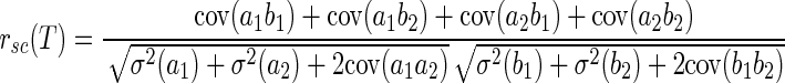(A2)

We made the following assumptions that are compatible with our data.

1. Variance: σ²(a₁) = σ²(a₂) = σ²(b₁) = σ²(b₂) = σ². Because we z-scored our data, σ² = 1.

2. Covariance between two neurons in a time interval: cov (a₁b₁) = cov (a₂b₂) = ϕ².

3. Cross-covariance between the responses of two neurons during different time intervals: cov (a₁b₂) = cov (a₂b₁) = ρ².

4. Autocovariance of an individual neuron: cov (a₁a₂) = cov (b₁b₂) = γ². Equation A2 can be simplified as

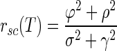(A3)

Spike count correlation for the intervals T_i, where i = [1, 2], is defined as

(A4)

Because the noise correlation is bounded at 1.0, the value of r_sc must reach an asymptote when the analysis interval is sufficiently long: r_sc(T) = r_sc(T_i) = r_eq. Substituting into this equality using Eqs. A3 and A4 yields

(A5)

implying that r_eq is reached if

(A6)

Rearrangement of Eq. A6 yields another way of describing the conditions where r_sc does not increase as a function of the duration of the analysis interval

(A7)

Now, consider the situation where r_sc(T) > r_sc(T_i). From Eqs. A3 and A4

(A8)

which is true only if

(A9)

meaning, if the denominators in (A8) and (A9) are positive, that

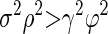(A10)

It follows that r_sc will grow (or not) as a function of the analysis interval in relation to the relative sizes of the left and right sides of Eq. A7.

In the strictest sense, Eqs. A1–A10 are valid only if the sensory stimulus is the same for every trial included in the analysis. Because the results reported in Table 2 are pooled across stimulus conditions, we repeated the analysis and found the same results when considering the data from single-stimulus conditions.

We can perform the same analysis for the effect of analysis window on the Fano factor. Again, consider a response interval T with two equal subintervals T₁ and T₂ and a neuron with responses a_i during the ith interval, where i = [1, 2]. Assume that the response variances and the means during the two subintervals are identical: σ₁² = σ₂² = σ²; μ₁ = μ₂ = μ. Then, the Fano factors (FF) during the two subintervals are the same

(A11)

For the longer time interval, T = T₁ + T₂

(A12)

Expanding the terms yields

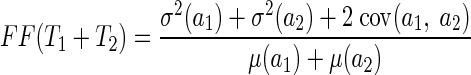(A13)

Combining terms and dividing top and bottom by 2 leads to

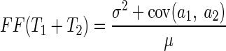(A14)

Therefore a positive autocovariance will lead to FF(T₁ + T₂) > FF(T₁), as we observed in our data and others have before (Osborne et al. 2004).

REFERENCES

Abbott and Dayan 1999.Abbott LF, Dayan P. The effect of correlated variability on the accuracy of a population code. Neural Comput 11: 91–101, 1999. [DOI] [PubMed] [Google Scholar]
Alonso et al. 2001.Alonso JM, Usrey WM, Reid RC. Rules of connectivity between geniculate cells and simple cells in cat primary visual cortex. J Neurosci 21: 4002–4015, 2001. [DOI] [PMC free article] [PubMed] [Google Scholar]
Averbeck et al. 2006.Averbeck BB, Latham PE, Pouget A. Neural correlations, population coding and computation. Nat Rev Neurosci 7: 358–366, 2006. [DOI] [PubMed] [Google Scholar]
Bair et al. 2001.Bair W, Zohary E, Newsome WT. Correlated firing in macaque visual area MT: time scales and relationship to behavior. J Neurosci 21: 1676–1697, 2001. [DOI] [PMC free article] [PubMed] [Google Scholar]
Bosking et al. 1997.Bosking WH, Zhang Y, Schofield B, Fitzpatrick D. Orientation selectivity and the arrangement of horizontal connections in tree shrew striate cortex. J Neurosci 17: 2112–2127, 1997. [DOI] [PMC free article] [PubMed] [Google Scholar]
Churchland and Lisberger 2001.Churchland MM, Lisberger SG. Shifts in the population response in the middle temporal visual area parallel perceptual and motor illusions produced by apparent motion. J Neurosci 21: 9387–9402, 2001. [DOI] [PMC free article] [PubMed] [Google Scholar]
Cohen and Newsome 2008.Cohen MR, Newsome WT. Context-dependent changes in functional circuitry in visual area MT. Neuron 60: 162–173, 2008. [DOI] [PMC free article] [PubMed] [Google Scholar]
de Bruyn and Orban 1988.de Bruyn B, Orban GA. Human velocity and direction discrimination measured with random dot patterns. Vision Res 28: 1323–1335, 1988. [DOI] [PubMed] [Google Scholar]
de la Rocha et al. 2007.de la Rocha J, Doiron B, Shea-Brown E, Josic K, Reyes A. Correlation between neural spike trains increases with firing rate. Nature 448: 802–806, 2007. [DOI] [PubMed] [Google Scholar]
de Oliveira et al. 1997.de Oliveira SC, Thiele A, Hoffmann KP. Synchronization of neuronal activity during stimulus expectation in a direction discrimination task. J Neurosci 17: 9248–9260, 1997. [DOI] [PMC free article] [PubMed] [Google Scholar]
Douglas and Martin 1991.Douglas RJ, Martin KA. A functional microcircuit for cat visual cortex. J Physiol 440: 735–769, 1991. [DOI] [PMC free article] [PubMed] [Google Scholar]
Gawne and Richmond 1993.Gawne TJ, Richmond BJ. How independent are the messages carried by adjacent inferior temporal cortical neurons? J Neurosci 13: 2758–2771, 1993. [DOI] [PMC free article] [PubMed] [Google Scholar]
Georgopoulos et al. 1986.Georgopoulos AP, Schwartz AB, Kettner RE. Neuronal population coding of movement direction. Science 233: 1416–1419, 1986. [DOI] [PubMed] [Google Scholar]
Gilbert and Wiesel 1983.Gilbert CD, Wiesel TN. Clustered intrinsic connections in cat visual cortex. J Neurosci 3: 1116–1133, 1983. [DOI] [PMC free article] [PubMed] [Google Scholar]
Groh et al. 1997.Groh JM, Born RT, Newsome WT. How is a sensory map read out? Effects of microstimulation in visual area MT on saccades and smooth pursuit eye movements. J Neurosci 17: 4312–4330, 1997. [DOI] [PMC free article] [PubMed] [Google Scholar]
Hubel and Wiesel 1962.Hubel DH, Wiesel TN. Receptive fields, binocular interaction and functional architecture in the cat's visual cortex. J Physiol 160: 106–154, 1962. [DOI] [PMC free article] [PubMed] [Google Scholar]
Jazayeri and Movshon 2006.Jazayeri M, Movshon JA. Optimal representation of sensory information by neural populations. Nat Neurosci 9: 690–696, 2006. [DOI] [PubMed] [Google Scholar]
Kohn and Smith 2005.Kohn A, Smith MA. Stimulus dependence of neuronal correlation in primary visual cortex of the macaque. J Neurosci 25: 3661–3673, 2005. [DOI] [PMC free article] [PubMed] [Google Scholar]
Lee et al. 1988.Lee C, Rohrer WH, Sparks DL. Population coding of saccadic eye movements by neurons in the superior colliculus. Nature 332: 357–360, 1988. [DOI] [PubMed] [Google Scholar]
Lee et al. 1998.Lee D, Port NL, Kruse W, Georgopoulos AP. Variability and correlated noise in the discharge of neurons in motor and parietal areas of the primate cortex. J Neurosci 18: 1161–1170, 1998. [DOI] [PMC free article] [PubMed] [Google Scholar]
Lisberger and Movshon 1999.Lisberger SG, Movshon JA. Visual motion analysis for pursuit eye movements in area MT of macaque monkeys. J Neurosci 19: 2224–2246, 1999. [DOI] [PMC free article] [PubMed] [Google Scholar]
Liu and Newsome 2005.Liu J, Newsome WT. Correlation between speed perception and neural activity in the middle temporal visual area. J Neurosci 25: 711–722, 2005. [DOI] [PMC free article] [PubMed] [Google Scholar]
Maunsell and Gibson 1992.Maunsell JH, Gibson JR. Visual response latencies in striate cortex of the macaque monkey. J Neurophysiol 68: 1332–1344, 1992. [DOI] [PubMed] [Google Scholar]
Maunsell and Van Essen 1983.Maunsell JH, Van Essen DC. Functional properties of neurons in middle temporal visual area of the macaque monkey. I. Selectivity for stimulus direction, speed, and orientation. J Neurophysiol 49: 1127–1147, 1983. [DOI] [PubMed] [Google Scholar]
McIlwain 1991.McIlwain JT Distributed spatial coding in the superior colliculus: a review. Vis Neurosci 6: 3–13, 1991. [DOI] [PubMed] [Google Scholar]
Medina and Lisberger 2007.Medina JF, Lisberger SG. Variation, signal, and noise in cerebellar sensory-motor processing for smooth-pursuit eye movements. J Neurosci 27: 6832–6842, 2007. [DOI] [PMC free article] [PubMed] [Google Scholar]
Michalski et al. 1983.Michalski A, Gerstein GL, Czarkowska J, Tarnecki R. Interactions between cat striate cortex neurons. Exp Brain Res 51: 97–107, 1983. [DOI] [PubMed] [Google Scholar]
Newsome et al. 1985.Newsome WT, Wurtz RH, Dursteler MR, Mikami A. Deficits in visual motion processing following ibotenic acid lesions of the middle temporal visual area of the macaque monkey. J Neurosci 5: 825–840, 1985. [DOI] [PMC free article] [PubMed] [Google Scholar]
Nover et al. 2005.Nover H, Anderson CH, DeAngelis GC. A logarithmic, scale-invariant representation of speed in macaque middle temporal area accounts for speed discrimination performance. J Neurosci 25: 10049–10060, 2005. [DOI] [PMC free article] [PubMed] [Google Scholar]
Oram et al. 1998.Oram MW, Földiák P, Perrett DI, Sengpiel F. The “Ideal Homunculus”: decoding neural population signals. Trends Neurosci 21: 259–265, 1998. [DOI] [PubMed] [Google Scholar]
Osborne et al. 2004.Osborne LC, Bialek W, Lisberger SG. Time course of information about motion direction in visual area MT of macaque monkeys. J Neurosci 24: 3210–3222, 2004. [DOI] [PMC free article] [PubMed] [Google Scholar]
Osborne et al. 2007.Osborne LC, Hohl SS, Bialek W, Lisberger SG. Time course of precision in smooth-pursuit eye movements of monkeys. J Neurosci 27: 2987–2998, 2007. [DOI] [PMC free article] [PubMed] [Google Scholar]
Osborne et al. 2005.Osborne LC, Lisberger SG, Bialek W. A sensory source for motor variation. Nature 437: 412–416, 2005. [DOI] [PMC free article] [PubMed] [Google Scholar]
Perkel et al. 1967.Perkel DH, Gerstein GL, Moore GP. Neuronal spike trains and stochastic point processes. II. Simultaneous spike trains. Biophys J 7: 419–440, 1967. [DOI] [PMC free article] [PubMed] [Google Scholar]
Pouget et al. 2000.Pouget A, Dayan P, Zemel R. Information processing with population codes. Nat Rev Neurosci 1: 125–132, 2000. [DOI] [PubMed] [Google Scholar]
Pouget et al. 2003.Pouget A, Dayan P, Zemel RS. Inference and computation with population codes. Annu Rev Neurosci 26: 381–410, 2003. [DOI] [PubMed] [Google Scholar]
Priebe et al. 2002.Priebe NJ, Churchland MM, Lisberger SG. Constraints on the source of short-term motion adaptation in macaque area MT. I. The role of input and intrinsic mechanisms. J Neurophysiol 88: 354–369, 2002. [DOI] [PMC free article] [PubMed] [Google Scholar]
Priebe and Lisberger 2004.Priebe NJ, Lisberger SG. Estimating target speed from the population response in visual area MT. J Neurosci 24: 1907–1916, 2004. [DOI] [PMC free article] [PubMed] [Google Scholar]
Ramachandran and Lisberger 2005.Ramachandran R, Lisberger SG. Normal performance and expression of learning in the vestibulo-ocular reflex (VOR) at high frequencies. J Neurophysiol 93: 2028–2038, 2005. [DOI] [PMC free article] [PubMed] [Google Scholar]
Rashbass 1961.Rashbass C The relationship between saccadic and smooth tracking eye movements. J Physiol 159: 326–338, 1961. [DOI] [PMC free article] [PubMed] [Google Scholar]
Reike et al. 1996.Reike F, Warland D, de Ruyter van Steveninck R, Bialek W. Spikes: Exploring the Neural Code. Cambridge, MA: MIT Press, 1996.
Schlack et al. 2007.Schlack A, Krekelberg B, Albright TD. Recent history of stimulus speeds affects the speed tuning of neurons in area MT. J Neurosci 27: 11009–11018, 2007. [DOI] [PMC free article] [PubMed] [Google Scholar]
Schoppmann and Hoffmann 1976.Schoppmann A, Hoffmann KP. Continuous mapping of direction selectivity in the cat's visual cortex. Neurosci Lett 2: 177–181, 1976. [DOI] [PubMed] [Google Scholar]
Series et al. 2004.Series P, Latham PE, Pouget A. Tuning curve sharpening for orientation selectivity: coding efficiency and the impact of correlations. Nat Neurosci 7: 1129–1135, 2004. [DOI] [PubMed] [Google Scholar]
Shadlen et al. 1996.Shadlen MN, Britten KH, Newsome WT, Movshon JA. A computational analysis of the relationship between neuronal and behavioral responses to visual motion. J Neurosci 16: 1486–1510, 1996. [DOI] [PMC free article] [PubMed] [Google Scholar]
Shadlen and Newsome 1994.Shadlen MN, Newsome WT. Noise, neural codes and cortical organization. Curr Opin Neurobiol 4: 569–579, 1994. [DOI] [PubMed] [Google Scholar]
Shamir and Sompolinsky 2004.Shamir M, Sompolinsky H. Nonlinear population codes. Neural Comput 16: 1105–1136, 2004. [DOI] [PubMed] [Google Scholar]
Smith and Kohn 2008.Smith MA, Kohn A. Spatial and temporal scales of neuronal correlation in primary visual cortex. J Neurosci 28: 12591–12603, 2008. [DOI] [PMC free article] [PubMed] [Google Scholar]
Snippe and Koenderink 1992.Snippe HP, Koenderink JJ. Information in channel-coded systems: correlated receivers. Biol Cybern 67: 183–190, 1992. [DOI] [PubMed] [Google Scholar]
Sompolinsky et al. 2001.Sompolinsky H, Yoon H, Kang K, Shamir M. Population coding in neuronal systems with correlated noise. Phys Rev E Stat Nonlin Soft Matter Phys 64: 051904, 2001. [DOI] [PubMed] [Google Scholar]
Sparks et al. 1976.Sparks DL, Holland R, Guthrie BL. Size and distribution of movement fields in the monkey superior colliculus. Brain Res 113: 21–34, 1976. [DOI] [PubMed] [Google Scholar]
Teich et al. 1996.Teich MC, Turcott RG, Siegel RM. Temporal correlation in cat striate-cortex neural spike trains. IEEE Eng Med Biol Mag 15: 79–87, 1996. [Google Scholar]
Ts'o et al. 1986.Ts'o DY, Gilbert CD, Wiesel TN. Relationships between horizontal interactions and functional architecture in cat striate cortex as revealed by cross-correlation analysis. J Neurosci 6: 1160–1170, 1986. [DOI] [PMC free article] [PubMed] [Google Scholar]
Weiss et al. 2002.Weiss Y, Simoncelli EP, Adelson EH. Motion illusions as optimal percepts. Nat Neurosci 5: 598–604, 2002. [DOI] [PubMed] [Google Scholar]
Zhang and Sejnowski 1999.Zhang K, Sejnowski TJ. Neuronal tuning: to sharpen or broaden? Neural Comput 11: 75–84, 1999. [DOI] [PubMed] [Google Scholar]
Zohary et al. 1994.Zohary E, Shadlen MN, Newsome WT. Correlated neuronal discharge rate and its implications for psychophysical performance. Nature 370: 140–143, 1994. [DOI] [PubMed] [Google Scholar]

[r1] Abbott and Dayan 1999.Abbott LF, Dayan P. The effect of correlated variability on the accuracy of a population code. Neural Comput 11: 91–101, 1999. [DOI] [PubMed] [Google Scholar]

[r2] Alonso et al. 2001.Alonso JM, Usrey WM, Reid RC. Rules of connectivity between geniculate cells and simple cells in cat primary visual cortex. J Neurosci 21: 4002–4015, 2001. [DOI] [PMC free article] [PubMed] [Google Scholar]

[r3] Averbeck et al. 2006.Averbeck BB, Latham PE, Pouget A. Neural correlations, population coding and computation. Nat Rev Neurosci 7: 358–366, 2006. [DOI] [PubMed] [Google Scholar]

[r4] Bair et al. 2001.Bair W, Zohary E, Newsome WT. Correlated firing in macaque visual area MT: time scales and relationship to behavior. J Neurosci 21: 1676–1697, 2001. [DOI] [PMC free article] [PubMed] [Google Scholar]

[r5] Bosking et al. 1997.Bosking WH, Zhang Y, Schofield B, Fitzpatrick D. Orientation selectivity and the arrangement of horizontal connections in tree shrew striate cortex. J Neurosci 17: 2112–2127, 1997. [DOI] [PMC free article] [PubMed] [Google Scholar]

[r6] Churchland and Lisberger 2001.Churchland MM, Lisberger SG. Shifts in the population response in the middle temporal visual area parallel perceptual and motor illusions produced by apparent motion. J Neurosci 21: 9387–9402, 2001. [DOI] [PMC free article] [PubMed] [Google Scholar]

[r7] Cohen and Newsome 2008.Cohen MR, Newsome WT. Context-dependent changes in functional circuitry in visual area MT. Neuron 60: 162–173, 2008. [DOI] [PMC free article] [PubMed] [Google Scholar]

[r8] de Bruyn and Orban 1988.de Bruyn B, Orban GA. Human velocity and direction discrimination measured with random dot patterns. Vision Res 28: 1323–1335, 1988. [DOI] [PubMed] [Google Scholar]

[r9] de la Rocha et al. 2007.de la Rocha J, Doiron B, Shea-Brown E, Josic K, Reyes A. Correlation between neural spike trains increases with firing rate. Nature 448: 802–806, 2007. [DOI] [PubMed] [Google Scholar]

[r10] de Oliveira et al. 1997.de Oliveira SC, Thiele A, Hoffmann KP. Synchronization of neuronal activity during stimulus expectation in a direction discrimination task. J Neurosci 17: 9248–9260, 1997. [DOI] [PMC free article] [PubMed] [Google Scholar]

[r11] Douglas and Martin 1991.Douglas RJ, Martin KA. A functional microcircuit for cat visual cortex. J Physiol 440: 735–769, 1991. [DOI] [PMC free article] [PubMed] [Google Scholar]

[r12] Gawne and Richmond 1993.Gawne TJ, Richmond BJ. How independent are the messages carried by adjacent inferior temporal cortical neurons? J Neurosci 13: 2758–2771, 1993. [DOI] [PMC free article] [PubMed] [Google Scholar]

[r13] Georgopoulos et al. 1986.Georgopoulos AP, Schwartz AB, Kettner RE. Neuronal population coding of movement direction. Science 233: 1416–1419, 1986. [DOI] [PubMed] [Google Scholar]

[r14] Gilbert and Wiesel 1983.Gilbert CD, Wiesel TN. Clustered intrinsic connections in cat visual cortex. J Neurosci 3: 1116–1133, 1983. [DOI] [PMC free article] [PubMed] [Google Scholar]

[r15] Groh et al. 1997.Groh JM, Born RT, Newsome WT. How is a sensory map read out? Effects of microstimulation in visual area MT on saccades and smooth pursuit eye movements. J Neurosci 17: 4312–4330, 1997. [DOI] [PMC free article] [PubMed] [Google Scholar]

[r16] Hubel and Wiesel 1962.Hubel DH, Wiesel TN. Receptive fields, binocular interaction and functional architecture in the cat's visual cortex. J Physiol 160: 106–154, 1962. [DOI] [PMC free article] [PubMed] [Google Scholar]

[r17] Jazayeri and Movshon 2006.Jazayeri M, Movshon JA. Optimal representation of sensory information by neural populations. Nat Neurosci 9: 690–696, 2006. [DOI] [PubMed] [Google Scholar]

[r18] Kohn and Smith 2005.Kohn A, Smith MA. Stimulus dependence of neuronal correlation in primary visual cortex of the macaque. J Neurosci 25: 3661–3673, 2005. [DOI] [PMC free article] [PubMed] [Google Scholar]

[r19] Lee et al. 1988.Lee C, Rohrer WH, Sparks DL. Population coding of saccadic eye movements by neurons in the superior colliculus. Nature 332: 357–360, 1988. [DOI] [PubMed] [Google Scholar]

[r20] Lee et al. 1998.Lee D, Port NL, Kruse W, Georgopoulos AP. Variability and correlated noise in the discharge of neurons in motor and parietal areas of the primate cortex. J Neurosci 18: 1161–1170, 1998. [DOI] [PMC free article] [PubMed] [Google Scholar]

[r21] Lisberger and Movshon 1999.Lisberger SG, Movshon JA. Visual motion analysis for pursuit eye movements in area MT of macaque monkeys. J Neurosci 19: 2224–2246, 1999. [DOI] [PMC free article] [PubMed] [Google Scholar]

[r22] Liu and Newsome 2005.Liu J, Newsome WT. Correlation between speed perception and neural activity in the middle temporal visual area. J Neurosci 25: 711–722, 2005. [DOI] [PMC free article] [PubMed] [Google Scholar]

[r23] Maunsell and Gibson 1992.Maunsell JH, Gibson JR. Visual response latencies in striate cortex of the macaque monkey. J Neurophysiol 68: 1332–1344, 1992. [DOI] [PubMed] [Google Scholar]

[r24] Maunsell and Van Essen 1983.Maunsell JH, Van Essen DC. Functional properties of neurons in middle temporal visual area of the macaque monkey. I. Selectivity for stimulus direction, speed, and orientation. J Neurophysiol 49: 1127–1147, 1983. [DOI] [PubMed] [Google Scholar]

[r25] McIlwain 1991.McIlwain JT Distributed spatial coding in the superior colliculus: a review. Vis Neurosci 6: 3–13, 1991. [DOI] [PubMed] [Google Scholar]

[r26] Medina and Lisberger 2007.Medina JF, Lisberger SG. Variation, signal, and noise in cerebellar sensory-motor processing for smooth-pursuit eye movements. J Neurosci 27: 6832–6842, 2007. [DOI] [PMC free article] [PubMed] [Google Scholar]

[r27] Michalski et al. 1983.Michalski A, Gerstein GL, Czarkowska J, Tarnecki R. Interactions between cat striate cortex neurons. Exp Brain Res 51: 97–107, 1983. [DOI] [PubMed] [Google Scholar]

[r28] Newsome et al. 1985.Newsome WT, Wurtz RH, Dursteler MR, Mikami A. Deficits in visual motion processing following ibotenic acid lesions of the middle temporal visual area of the macaque monkey. J Neurosci 5: 825–840, 1985. [DOI] [PMC free article] [PubMed] [Google Scholar]

[r29] Nover et al. 2005.Nover H, Anderson CH, DeAngelis GC. A logarithmic, scale-invariant representation of speed in macaque middle temporal area accounts for speed discrimination performance. J Neurosci 25: 10049–10060, 2005. [DOI] [PMC free article] [PubMed] [Google Scholar]

[r30] Oram et al. 1998.Oram MW, Földiák P, Perrett DI, Sengpiel F. The “Ideal Homunculus”: decoding neural population signals. Trends Neurosci 21: 259–265, 1998. [DOI] [PubMed] [Google Scholar]

[r31] Osborne et al. 2004.Osborne LC, Bialek W, Lisberger SG. Time course of information about motion direction in visual area MT of macaque monkeys. J Neurosci 24: 3210–3222, 2004. [DOI] [PMC free article] [PubMed] [Google Scholar]

[r32] Osborne et al. 2007.Osborne LC, Hohl SS, Bialek W, Lisberger SG. Time course of precision in smooth-pursuit eye movements of monkeys. J Neurosci 27: 2987–2998, 2007. [DOI] [PMC free article] [PubMed] [Google Scholar]

[r33] Osborne et al. 2005.Osborne LC, Lisberger SG, Bialek W. A sensory source for motor variation. Nature 437: 412–416, 2005. [DOI] [PMC free article] [PubMed] [Google Scholar]

[r34] Perkel et al. 1967.Perkel DH, Gerstein GL, Moore GP. Neuronal spike trains and stochastic point processes. II. Simultaneous spike trains. Biophys J 7: 419–440, 1967. [DOI] [PMC free article] [PubMed] [Google Scholar]

[r35] Pouget et al. 2000.Pouget A, Dayan P, Zemel R. Information processing with population codes. Nat Rev Neurosci 1: 125–132, 2000. [DOI] [PubMed] [Google Scholar]

[r36] Pouget et al. 2003.Pouget A, Dayan P, Zemel RS. Inference and computation with population codes. Annu Rev Neurosci 26: 381–410, 2003. [DOI] [PubMed] [Google Scholar]

[r37] Priebe et al. 2002.Priebe NJ, Churchland MM, Lisberger SG. Constraints on the source of short-term motion adaptation in macaque area MT. I. The role of input and intrinsic mechanisms. J Neurophysiol 88: 354–369, 2002. [DOI] [PMC free article] [PubMed] [Google Scholar]

[r38] Priebe and Lisberger 2004.Priebe NJ, Lisberger SG. Estimating target speed from the population response in visual area MT. J Neurosci 24: 1907–1916, 2004. [DOI] [PMC free article] [PubMed] [Google Scholar]

[r39] Ramachandran and Lisberger 2005.Ramachandran R, Lisberger SG. Normal performance and expression of learning in the vestibulo-ocular reflex (VOR) at high frequencies. J Neurophysiol 93: 2028–2038, 2005. [DOI] [PMC free article] [PubMed] [Google Scholar]

[r40] Rashbass 1961.Rashbass C The relationship between saccadic and smooth tracking eye movements. J Physiol 159: 326–338, 1961. [DOI] [PMC free article] [PubMed] [Google Scholar]

[r41] Reike et al. 1996.Reike F, Warland D, de Ruyter van Steveninck R, Bialek W. Spikes: Exploring the Neural Code. Cambridge, MA: MIT Press, 1996.

[r42] Schlack et al. 2007.Schlack A, Krekelberg B, Albright TD. Recent history of stimulus speeds affects the speed tuning of neurons in area MT. J Neurosci 27: 11009–11018, 2007. [DOI] [PMC free article] [PubMed] [Google Scholar]

[r43] Schoppmann and Hoffmann 1976.Schoppmann A, Hoffmann KP. Continuous mapping of direction selectivity in the cat's visual cortex. Neurosci Lett 2: 177–181, 1976. [DOI] [PubMed] [Google Scholar]

[r44] Series et al. 2004.Series P, Latham PE, Pouget A. Tuning curve sharpening for orientation selectivity: coding efficiency and the impact of correlations. Nat Neurosci 7: 1129–1135, 2004. [DOI] [PubMed] [Google Scholar]

[r45] Shadlen et al. 1996.Shadlen MN, Britten KH, Newsome WT, Movshon JA. A computational analysis of the relationship between neuronal and behavioral responses to visual motion. J Neurosci 16: 1486–1510, 1996. [DOI] [PMC free article] [PubMed] [Google Scholar]

[r46] Shadlen and Newsome 1994.Shadlen MN, Newsome WT. Noise, neural codes and cortical organization. Curr Opin Neurobiol 4: 569–579, 1994. [DOI] [PubMed] [Google Scholar]

[r47] Shamir and Sompolinsky 2004.Shamir M, Sompolinsky H. Nonlinear population codes. Neural Comput 16: 1105–1136, 2004. [DOI] [PubMed] [Google Scholar]

[r48] Smith and Kohn 2008.Smith MA, Kohn A. Spatial and temporal scales of neuronal correlation in primary visual cortex. J Neurosci 28: 12591–12603, 2008. [DOI] [PMC free article] [PubMed] [Google Scholar]

[r49] Snippe and Koenderink 1992.Snippe HP, Koenderink JJ. Information in channel-coded systems: correlated receivers. Biol Cybern 67: 183–190, 1992. [DOI] [PubMed] [Google Scholar]

[r50] Sompolinsky et al. 2001.Sompolinsky H, Yoon H, Kang K, Shamir M. Population coding in neuronal systems with correlated noise. Phys Rev E Stat Nonlin Soft Matter Phys 64: 051904, 2001. [DOI] [PubMed] [Google Scholar]

[r51] Sparks et al. 1976.Sparks DL, Holland R, Guthrie BL. Size and distribution of movement fields in the monkey superior colliculus. Brain Res 113: 21–34, 1976. [DOI] [PubMed] [Google Scholar]

[r52] Teich et al. 1996.Teich MC, Turcott RG, Siegel RM. Temporal correlation in cat striate-cortex neural spike trains. IEEE Eng Med Biol Mag 15: 79–87, 1996. [Google Scholar]

[r53] Ts'o et al. 1986.Ts'o DY, Gilbert CD, Wiesel TN. Relationships between horizontal interactions and functional architecture in cat striate cortex as revealed by cross-correlation analysis. J Neurosci 6: 1160–1170, 1986. [DOI] [PMC free article] [PubMed] [Google Scholar]

[r54] Weiss et al. 2002.Weiss Y, Simoncelli EP, Adelson EH. Motion illusions as optimal percepts. Nat Neurosci 5: 598–604, 2002. [DOI] [PubMed] [Google Scholar]

[r55] Zhang and Sejnowski 1999.Zhang K, Sejnowski TJ. Neuronal tuning: to sharpen or broaden? Neural Comput 11: 75–84, 1999. [DOI] [PubMed] [Google Scholar]

[r56] Zohary et al. 1994.Zohary E, Shadlen MN, Newsome WT. Correlated neuronal discharge rate and its implications for psychophysical performance. Nature 370: 140–143, 1994. [DOI] [PubMed] [Google Scholar]

PERMALINK

Noise Correlations in Cortical Area MT and Their Potential Impact on Trial-by-Trial Variation in the Direction and Speed of Smooth-Pursuit Eye Movements

Xin Huang

Stephen G Lisberger

Abstract

INTRODUCTION

METHODS

Data acquisition, behavioral paradigm, and visual stimuli

Experimental design

Correlation analysis

Other analyses

Computer simulations of MT population responses

Decoding model

RESULTS

FIG. 1.

Computational analysis of the general effect of correlations between neurons on variation in estimates of target speed and direction

Physiology database and correlation between responses of an exemplar MT neuron pair

FIG. 2.

Effect of randomizing the dot pattern on neuronal correlation

FIG. 3.

FIG. 10.

Structure of noise correlations in MT

TABLE 1.

FIG. 4.

FIG. 5.

Time course of noise correlation in MT

FIG. 6.

Time interval of neural response and noise correlation

FIG. 7.

TABLE 2.

Speed dependence of noise correlations in MT

FIG. 8.

FIG. 9.

Contrast dependence of noise correlations in MT

Decoding stimulus speed and direction from MT population responses

FIG. 11.

FIG. 12.

FIG. 13.

Population responses that capture the variation of pursuit eye movements in specific subjects

DISCUSSION

Properties of noise correlation

Implications of noise correlations for the coding of visual motion in MT

Implications of correlations for decoding motion signals from MT population responses

Sensory noise, population decoding, and behavioral variation

GRANTS

Acknowledgments

APPENDIX

REFERENCES

ACTIONS

PERMALINK

RESOURCES

Similar articles

Cited by other articles

Links to NCBI Databases