Analyzing Variability in Neural Responses to Complex Natural Sounds in the Awake Songbird

Abstract

Studies of auditory processing in awake, behaving songbirds allow for the possibility of new classes of experiments, including those involving attention and plasticity. Detecting and determining the significance of plasticity, however, requires assessing the intrinsic variability in neural responses. Effects such as rapid plasticity have been investigated in the auditory system through the use of the spectrotemporal receptive field (STRF), a characterization of the properties of sounds to which a neuron best responds. Here we investigated neural response variability in awake recordings obtained from zebra finch field L, the analog of the primary auditory cortex. To quantify the level of variability in the neural recordings, we used three similarity measures: an STRF-based metric, a spike-train correlation-based metric, and a spike-train discrimination-based metric. We then extracted a number of parameters from these measures, quantifying how they fluctuated over time. Our results indicate that 1) awake responses are quite stable over time; 2) the different measures of response are complementary—specifically, the spike-train–based measures yield new information complementary to the STRF; and 3) different STRF parameters show distinct levels of variability. These results provide critical constraints for the design of robust decoding strategies and novel experiments on attention and plasticity in the awake songbird.

INTRODUCTION

An animal's accurate responses to natural stimuli are often essential to its survival. The study of how these stimuli are encoded and processed at the neural level should provide insight into the fundamental problem of neural coding. Of specific interest are natural sounds, which display intricate time-varying structure over multiple timescales (Attias and Schreiner 1998; Escabí et al. 2003; Lewicki 2002; Nelken et al. 1999; Singh and Theunissen 2003) that provide important cues for sound recognition. Previous studies have suggested that the auditory cortex plays an important role in the processing of natural auditory scenes and species-specific vocalizations (Fitch et al. 1997; Nelken 2004; Rauschecker 1998; Wang 2000).

Songbirds provide a model system that offers unique advantages for studying the processing of complex sounds (Doupe and Kuhl 1999). As with other animal species, songbirds communicate using a set of acoustically complex vocalizations that transmit behaviorally relevant information important for intraspecies interactions such as descriptions of the identity and location of the sender (Konishi 1985; Theunissen et al. 2000; Wang 2000). Field L, the avian analog of the auditory cortex, is selective to conspecific vocalizations and is thought to play an important role in the processing and discrimination of these sounds (Grace et al. 2003; Sen et al. 2001; Theunissen et al. 2000, 2004).

How does one assess the variability of neural recordings? The awake system allows for the investigation of both attentional effects and rapid, on-line plasticity, but is subjected to neural response variability over time. Thus answering this question is vital to understanding and validating the results of long-term neurophysiological experiments, including short-term plasticity effects caused by behavioral training (Eggermont 2006; Fritz et al. 2003; Spierer et al. 2007; Weinberger et al. 2006). An accurate assessment of the variability of neural responses also allows for the development of robust decoding strategies. To answer this question, we chose to investigate the spectrotemporal receptive field (STRF), a widely used characterization of the spectral and temporal features of sounds to which neurons best respond (Escabí and Schreiner 2002; Sen et al. 2001; Theunissen et al. 2000). An elegant set of studies have used the STRF to investigate rapid plasticity in neural responses, revealing dramatic task-dependent plasticity in the primary auditory cortex (Elhilali et al. 2007; Fritz et al. 2003, 2005). Here we obtain STRFs in awake restrained zebra finch field L using complex natural sounds, specifically conspecific (same species) vocalizations, and investigate the intrinsic variability of STRFs over time, up to several hours.

We also use two other response measures: a spike-train correlation-based metric and a spike-train discrimination metric (Billimoria et al. 2008; Larson et al. 2009; Narayan et al. 2006; Wang et al. 2007) to quantify variability. We address several questions: 1) how stable is the STRF over time, 2) do other quantitative measures of response yield complementary information on response variability, and 3) do different parameters of the STRF show identical levels of variability?

METHODS

Surgical procedures

We recorded from the field L region of awake adult male zebra finches (Taeniopygia guttata). All procedures were in strict accordance with the National Institutes of Health guidelines as approved by the Boston University Charles River Campus Institutional Animal Care and Use Committee. Two days prior to the electrophysiological recording, the bird was anesthetized (0.1–4% isoflurane in 0.5–2.5 l/min O₂) for a preparatory surgical procedure to implant a manually operated microdrive and fix a head-support pin. A reference point for electrode penetrations was marked with ink 1.5 mm lateral and 1.2 mm anterior to the bifurcation point of the midsagittal sinus. A lightweight microdrive containing two extracellular tungsten electrodes (impedance: 2–4 MΩ; FHC, Bowdoin, ME) was positioned above the marked dot. The microdrive was a modified version of a previous device used to record from awake zebra finches (Hessler and Doupe 1999). The skull and dura beneath the dot were removed and the implant was positioned such that the electrodes just entered the brain. The implant was secured to the skull in this configuration with epoxy. A reference ground electrode was inserted into the brain on the opposite hemisphere from the location of the implant. Finally, a steel support pin was glued to the skull above the midsagittal sinus. The bird was allowed to recover for 2 days before performing the experiments.

Stimuli

The stimulus ensemble played to the subjects consisted of 20 undirected, conspecific zebra finch songs recorded in a sound-attenuated chamber (Acoustic Systems, Austin, TX). The songs were sampled at 32 kHz, band-pass filtered to retain frequencies between 250 Hz and 8 kHz, and stored in data files for playback (Sen et al. 2001).

Electrophysiology

On the day of the experiment, the bird was restrained in a small cloth jacket to limit movement and reduce motion artifacts; the bird was then positioned in a stereotactic assembly and placed into a double-walled sound-attenuated chamber (Industrial Acoustics, Bronx, NY), facing a loudspeaker that was used for stimulus presentation. The speaker was located 20 cm away from the beak and the bird was elevated to be at the same height as the center of the speaker cone. The bird's head position was fixed by attaching the steel pin to a frame located on the stereotactic assembly; this served to further reduce the incidents of motion artifacts in the recordings. Single- and multiunit complexes in the same adult zebra finch were probed by manually advancing the two tungsten electrodes via the microdrive in roughly 150-μm intervals and playing a conspecific song that was not part of the test stimulus ensemble. The bird was given a 30-min break after each recording session not lasting >3 h and released from the cloth jacket into its cage. Data from a particular site were obtained within the same recording session; occasionally, some sites were probed and responses recorded over two or more successive sessions. Different sites were sampled over several days to weeks. After the experiment was concluded, the bird was killed with an overdose of isoflurane and the brain was preserved in 3.7% formalin fixative for histology.

Histology

Prior to sectioning, the brains were stored overnight in 30% sucrose buffer. Parasagittal 50-μm sections of the brain were prepared using a cryo-microtome and stained with cresyl violet (Nissl stain). Electrode placement was verified by comparing electrode tracks and electrolytic lesions to histological markers that define the boundaries of field L (Fortune and Margoliash 1992). Sites were classified as field L sites based on a combination of histology, medial–lateral coordinates, and depth of the recording site.

Neural data

Data were analyzed for STRF calculation only for sites that exhibited an average firing rate that was significantly different (P < 0.001, paired t-test) from the average spontaneous firing rate for at least one song stimulus. At a number of these sites, we obtained multiple recording blocks, defined as the interleaved presentation of 10 trials each of 20 conspecific zebra finch songs. Each recording block was presented ≥20 min after the start of the previous recording block for a particular site. Recording sessions were terminated early if the subject became restless or if 3 h had expired. In this manner, neural data were obtained from 28 sites in nine birds. Trials that demonstrated motion artifacts were removed from the data sets, although these constituted only a small number of the total number of trials (∼0.5%).

Spike sorting and data analysis were performed using custom software written in Matlab (The MathWorks, Natick, MA). Spike event times were obtained from the spike waveforms using a visually determined threshold and a window discriminator; the same threshold was used for spike event times across multiple recordings from a particular electrode depth and bird. Classification of sites into multiunits followed the scheme used in Sen et al. (2001). Multiunits consisted of spike waveforms that could be easily distinguished from the background noise, but not from each other, and contained small clusters of neurons.

STRF calculation

A detailed description of the calculation of STRFs from natural sounds can be found in Theunissen et al. (2000). A STRF can be defined as the optimal linear filter that transforms a particular representation of a time-varying stimulus into a prediction of a neuron's firing rate. Calculations were performed using the STRFPAK software suite (Zhang et al. 2006), which uses an invertible spectrographic representation of the sound stimuli and finds the optimal linear filter that, when convolved with the spectrographic representations of the stimuli, best matches the predicted firing of the recording site. This method corrects for the spectral and temporal correlations present in the sounds by performing a calculation that normalizes the song spike-train correlation by the autocorrelation of the stimuli. The resultant STRF is presented with limited resolution in the spectral and temporal domains, both as a result of the calculations performed and limited by the resolution of the inputs; in particular, the spectral resolution is 250 Hz (the bandwidth of the filter banks used to decompose the song spectrogram) and the temporal bin width is 1 ms (because the sampling rate of the spike trains is 1 kHz).

To determine the significant regions in the STRFs obtained, a jackknife resampling method was used (Sen et al. 2001); STRFs were calculated for multiple subsets of the conspecific song ensemble, obtained by deleting one song at a time from the entire ensemble. The variance for each spectrotemporal bin in the STRF estimate was calculated from this set of STRFs; the SE was obtained by taking the square root of the variance and was plotted on the STRF images.

The STRF was denoised using singular-valued decomposition (SVD). Singular values were calculated for the causal (0 to 100 ms) and acausal (−150 to −50 ms) regions of the STRF. The singular values from the causal region greater than the maximum singular value from the acausal region were used to reconstruct a denoised STRF. We also calculated the signal-to-noise ratio (SNR) of this denoised STRF by dividing the power in this causal region by the power in the acausal region.

STRF-based similarity index

We quantified the level of variability between two STRFs calculated from different recording blocks at the same site using a similarity index (SI) (DeAngelis et al. 1999; Escabí and Schreiner 2002). First, the STRFs in question were treated as vectors by reading the values from each matrix down its columns. These vectorized STRFs were then used to calculate the similarity index

where 〈, 〉 is the vector inner product and |·| is the vector norm operator. Values of SI close to 1 indicate strong similarity between the two STRFs. The SI is calculated between the first STRF and any successive STRFs obtained from the recording site under investigation.

Correlation-based similarity: R_corr

To more robustly assess the variability in subsequent recordings, we used two more computational measures derived directly from the neural recordings, as opposed to the STRFs. The first of these, called R_corr, is based on a previously described correlation-based measure of spike similarity (Schreiber et al. 2003). The similarity between two spike trains r→_i and r→_j is calculated as follows

where s→_i and s→_j were obtained by filtering r→_i and r→_j, respectively, using a Gaussian filter with mean 0 and SD 10 ms. An R_corr value close to 1 indicates similarity between the spike trains, whereas a value close to 0 indicates dissimilarity. Averaging the values of R_corr over the different pairs of spike trains obtained in one recording yields a measure of the reliability of the unit in responding to different stimuli.

We used the R_corr measure in two ways. First, as described in the previous section, we calculated R_corr as the reliability of responses obtained within recording blocks. Second, we adapted R_corr to quantify the similarity between sets of neural responses obtained across recording blocks at the same site. To adapt the R_corr measure for this series of calculations, r→_i and r→_j represent spike trains resulting from presentation of the same stimulus but obtained from different recording blocks at the same site. As for the STRF similarity index, the calculation was also performed between spike trains in the first recording block and spike trains in each of the subsequent recording blocks. The resulting R_corr values are then averaged over the trials and songs to obtain a measure of spike-train similarity across the two recordings blocks.

Performance-based similarity

The second similarity measure derived directly from the neural data is based on a previously described spike distance metric (SDM) (Narayan et al. 2006; van Rossum 2001). First, spike trains were filtered using a decaying exponential kernel with time constant τ

where t_i is the ith spike time, M is the total number of spikes given a spike train length T, and H(t) is the Heaviside step function. The spike distance is then computed between a pair of filtered spike trains f and g

By varying τ, discrimination could be measured over different timescales of the neural response. At short timescales, the metric acts like a coincidence detector, with small differences in spike timing contributing to the distance, whereas at long timescales, the metric acts like a rate difference counter, where average firing rates contribute to the distance.

A classification scheme based on the SDM was then used to quantify the neural discrimination of songs (Machens et al. 2003). Ten trials of spike trains were obtained from the recording for each of the 20 songs aligned at their onsets. A template spike train was chosen for each song and the remaining spike trains were assigned to the song with the closest template based on the spike distance measure. This procedure was repeated 1,000 times for different templates. Discrimination performance was quantified by computing the percentage of correctly classified songs (% correct). The chance level for classification is 5%, since a spike train could be assigned to 1 of 20 songs.

As with R_corr, a percentage correct was calculated in two ways for the various recordings obtained from a particular neural unit. The first was as described earlier, selecting template spike trains and assigning spike trains from the same recording block. Second, the metric was adapted to act as another measure to quantify the similarity between neural responses in blocks from the same recording site. For this set of calculations, f and g are filtered spike trains from two different recording blocks; the first recording block made at a particular site is the reference f and g is the set of responses from each subsequent recording block obtained at that site (e.g., distances are calculated between spike trains from the first recording block and the second recording block, then from the first recording block and the third recording block, and so on). The value of τ was chosen to reflect the optimal timescale observed in previous experiments (Narayan et al. 2006; Wang et al. 2007); the SD in the preceding R_corr calculations was chosen to coincide with this value. The parameters for calculating the distances were fixed, with τ at 10 ms and a spike-train length of 1,000 ms. The template songs were then chosen from the spike trains of the first recording block and spike trains from the subsequent recording blocks are matched to this template. This procedure was repeated for 1,000 different permutations of template songs, generating a percentage correct of correctly classified songs.

Analysis of STRF parameters

We also analyzed STRF similarity by studying the changes in six parameters derived from the STRF as described previously (Sen et al. 2001). Briefly, these parameters are latency; the time of the peak amplitude in the STRF; the center frequency (CF); the frequency of the peak amplitude in the STRF; the quality factor (Q), a measure of the sharpness of this spectral peak; the excitatory–inhibitory ratio (EIR), which gives an estimate of the concentration of the excitatory and inhibitory energies in the STRF; the separability index (SI), a term derived from the singular value decomposition of the STRF, which quantifies the time–frequency separability of the filter; and the temporal integration window (TiW), which estimates the temporal characteristic of the neuron that processes the amplitude envelope of sound. One difference between the sets of parameters obtained is in choosing the temporal integration window over the best modulation frequency (BMF, the frequency showing the highest value in the power-spectral density obtained from a temporal slice obtained at the center frequency) which was used in Sen et al. We observed that, for individual recordings at many neural sites, the multiple jackknife estimates showed high variability in their BMF, so we instead opted to use the temporal integration window, which gives similar information. Note that the time–frequency resolution chosen for the STRF, which was the same resolution used in prior work on field L (Sen et al. 2001; Theunissen et al. 2000), affects the resolution of the parameters extracted from the STRF. In particular, the minimum detectable change for the CF is 250 Hz as a result of the filter banks chosen. This results in a 16.7% change, for example, if the initial CF is 1,500 Hz.

RESULTS

Similarity index

We performed a total of 94 recordings from 28 sites in nine zebra finches. For each of these recordings, STRFs were calculated and compared using the similarity index measure described earlier. Figure 1, A–D shows four STRF plots obtained from one neural recording site. Areas in red indicate excitatory subregions, whereas areas in blue indicate inhibitory subregions. Dotted contours show 1SD and solid contours show 2SDs away from the mean STRF. The time stamp in the top right corner of each STRF plot indicates the time elapsed after the start of the first recording block obtained at the site. The four STRFs share qualitatively similar features, e.g., the time and frequency of the main excitatory subregion, with the shapes of the significant regions as depicted by the contours.

FIG. 1.

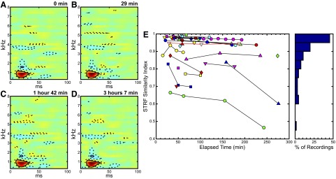
The majority of field L spectrotemporal receptive fields (STRFs) show high similarity across time as measured by the STRF similarity index (SI). A–D: STRF plots obtained from a particular neural recording site; time stamps at the top right corner of each STRF plot indicate the time elapsed after the start of the 1st recording block obtained at that same site. Warmer colors indicate excitatory regions and cooler colors inhibitory regions. E: plot of the STRF SI performed on all sites where multiple recordings were performed, plotted against the time elapsed after the start of the 1st recording block obtained at each site. Values of the SI for the site shown in A–D are outlined in red. To the right, a histogram shows the data in bins of size 0.05.

One of our goals was to use the information found in the STRF to derive a STRF similarity measure to analyze variability in the awake neural recordings. A majority of the recording sites showed high similarity over varying lengths of time as measured by the STRF SI. Figure 1E shows a graph of the SIs calculated between the first STRF and all subsequent STRFs for a particular recording site plotted against the time elapsed after the start of the first recording block obtained at each site with more similar STRFs having a similarity index closer to a value of one. The site depicted in Fig. 1, A–D is outlined in red and different sites are distinguished by a unique color/shape pair. On the right of the graph, a histogram shows the similarity index data binned in groups of 0.05, highlighting the number of STRFs for which there was a high similarity index. The mean value of the SIs was 0.90 with SE of 0.01. We also calculated the percentage change in STRF similarity index values for sites where more than two recording blocks were obtained. The mean percentage change in STRF similarity index was −3.2%, with SE of 1.2%.

Although a number of recording sites demonstrated qualitatively similar STRFs across recording blocks, there was a small number of sites where the STRF varied considerably across time. Supplemental Fig. S1 shows an example of a variable STRF.1 The time stamps above each plot show the time of the recording relative to the start time of the first STRF. Text in the top left corner of each plot indicates the SI calculated between that STRF and the first STRF shown; these numbers are plotted with the upward-pointing, blue triangle symbols in Fig. 1.

Correlation-based similarity: R_corr

Response similarity was also quantified using the R_corr measure described earlier. Specifically, we calculated R_corr using pairs of neural recordings and plotted the results in Fig. 2. Figure 2, A–D shows four sets of 10 spike rasters each; these rasters correspond to the STRF plots in Fig. 1. The time stamps above each set of rasters denote the time elapsed after the start of the first recording block at that site. Across both single-block trial recordings and the four recording blocks, the spike rasters show reproducible firing in response to the stimulus across a span of >3 h.

FIG. 2.

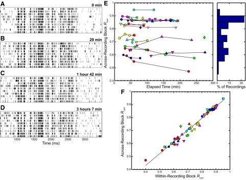
Illustration of spike-correlation–based similarity (R_corr) over time. A–D: raster plots from the site whose STRFs are depicted in Fig. 1, A–D; time stamps at the top right corner of each raster plot indicate the time elapsed after the start of the 1st recording block obtained at the same site. E: plot of across-recording block R_corr, where R_corr was calculated between the responses from the 1st recording block and the responses from each subsequent recording block at a particular site plotted against the time elapsed after the start of the 1st recording block obtained at each site. To the right, a histogram shows the same data in bins of size 0.05. F: comparison of within-recording block R_corr to across-recording block R_corr, with a best-fit line plotted in black. The correlation coefficients was 0.98 (P < 0.001). In panels (E) and (F), the values of R_corr for the data shown in (A–D) are outlined in red.

We also quantified the similarity in these spike trains by calculating the R_corr variability measure across recording blocks. Across the spike trains for all of the different recording sites, we observed low variability using the across-recording block R_corr measure over time. Figure 2E shows a plot of the R_corr measure calculated between the responses from the first recording block and the responses from each subsequent recording block at a particular site plotted against the time elapsed after the start of the first recording block for each site. A maximal value of one indicates perfect correlation. The example site depicted in Fig. 2, A–D is outlined in red and different sites are distinguished by a unique color/shape pair corresponding to the color/shape pair shown in Fig. 1E. On the right of the plot, a histogram shows the across-recording block R_corr data binned in groups of 0.05. The histogram indicates a more spread out distribution of values compared with the SIs. The mean value of R_corr was 0.76 with SE of 0.01. We also calculated the percentage change in across-recording block R_corr for sites where more than two recording blocks were obtained. The mean percentage change in across-recording block R_corr was −1.7%, with SE of 0.8%.

To better understand the source of variability observed in the R_corr values, we plotted across-recording block R_corr against within-recording block R_corr in Fig. 2F. For each site, we plotted all but the first within-recording site R_corr value against the corresponding across-recording block R_corr values because there is one less across-recording block value. A black line is plotted as the best-fit estimation between the data; the correlation coefficient was 0.98 (P < 0.001).

Performance-based similarity

The third similarity measure used was based on the discrimination performance algorithm described earlier using the van Rossum metric. Many of the recording sites show low variability using the performance-based measure as indicated by similar values of the measure over time. Figure 3A shows a graph of the discrimination performance calculated between the responses from the first recording block and the responses from each subsequent recording block at a particular site plotted against the time elapsed after the start of the first recording block obtained at the same site. The site depicted in Fig. 1, A–D is outlined in red and different sites are distinguished by a unique color/shape pair corresponding to the color/shape pair shown in Fig. 1E. On the right, a histogram shows the distribution of across-recording block discrimination values binned in groups of 5%. As with the R_corr histogram, the values of the discrimination performance-based similarity values are more spread out than the SI values. The mean value of the discrimination performance was 64.87% with SE of 3.992%. As with STRF SI and R_corr, we calculated the percentage change in the performance-based similarity measure for sites where more than two recording blocks were obtained. The mean percentage change was 0.3%, with SE of 4.9%.

FIG. 3.

Discrimination-performance–based similarity shows relative stability over time at most sites. A: plot of across-recording block performance, where the discrimination performance was calculated between the responses from the 1st recording block and the responses from each subsequent recording block at a particular site plotted against the time elapsed after the start of the 1st recording block obtained at the same site. To the right, a histogram shows the same data in bins of 5%. B: comparison of within-recording block performance to across-recording block performance, with a best-fit line plotted in black. The correlation coefficient was 0.95 (P < 0.001). The values of performance for the example data shown in Figs. 1 and 2, A–D are outlined in red.

We plotted across-recording block performance against within-recording block performance in Fig. 3B. As with the R_corr calculations, for each site we obtained one more within-recording block measure than we did for the across-recording block calculation, and so we plotted all but the first within-recording block performance value against the corresponding across-recording block performance values. A black line is plotted as the best-fit estimation between the data; the correlation coefficient was 0.95 (P < 0.001).

Comparing the similarity measures

We quantified the relationship among across-recording block R_corr, the performance-based similarity measure, and the STRF SI by plotting one against the other in Fig. 4, showing that the three measures were highly correlated. Figure 4A shows the relationship between the performance-based similarity and R_corr; a least-squares linear fit yielded the line in black; the correlation coefficient was found to be 0.95 (P < 0.001). Figure 4B shows the comparison between across-recording block discrimination performance and the STRF SI; the correlation coefficient between these two measures was 0.69 (P < 0.001). Finally, Fig. 4C shows across-recording block R_corr versus STRF SI; the correlation coefficient was 0.66 (P < 0.001). One recording site in particular, indicated by the red-filled circles, showed a marked difference between the two spike-variability measures, with high values for the STRF SI but lower values for the R_corr measure and the performance-based measure. The STRFs for this recording site demonstrated qualitatively similar features across the recording blocks but showed a decrease in the absolute intensities of the peaks with time. This is further reflected in the spike rasters, which showed a decrease in the overall firing rate across recording blocks.

FIG. 4.

R_corr and performance-based similarity are more correlated to each other than either is to the STRF SI. A: plot of across-recording block discrimination performance vs. across-recording block R_corr data. A best-fit line is plotted in black; the correlation coefficient between the 2 measures was 0.95 (P < 0.001). B: plot of across-recording block discrimination performance from Fig. 3 vs. the STRF SI. The correlation coefficient was 0.69 (P < 0.001). C: plot comparing across-recording block R_corr data from Fig. 2E to the STRF SI from Fig. 1. The correlation coefficient was 0.66 (P < 0.001). The data from the example site in Figs. 1 and 2 are outlined in red.

We also calculated the signal-to-noise ratio (SNR) for the STRF, comparing the power in the acausal region (defined as the STRF data between −150 and −50 ms) to that in the causal region (defined as the STRF data between 0 and 100 ms) and compared the results to the three similarity measures. Supplemental Fig. S2 shows the SNR plotted in decibels for the second and subsequent STRFs obtained from a particular recording site plotted against the similarity indices calculated previously. The solid black line represents a significant correlation between the SNR and the SI (r = 0.60, P < 0.001). We also compared the SNR to both the R_corr and performance-based measures; both correlations were smaller and less significant than the one comparing the SNR and the STRF SI (R_corr: r = 0.29, P = 0.018; performance measure: r = 0.35, P < 0.004; data not shown).

STRF parameters

We extracted a set of six parameters to characterize the STRF, providing an additional measure of similarity to compare multiple neural recordings from a particular site.

The parameters are summarized in the plots of Fig. 5. Each panel shows one of the six parameters plotted against the elapsed time since the first neural recording, with different units designated by different color/shape pairs. As before, the data corresponding to the example site featured in the figures are outlined in red. Percentage changes in these parameters, taken relative to the first recording for each site, are presented in Table 1. The plots demonstrate a wide range of values for the different parameters, indicative of the large variety of STRFs obtained in the study. Further, qualitative inspection of the parameters indicates that three of the six—latency, excitatory–inhibitory ratio, and separability index—did not widely vary across recording times. The temporal integration window showed modest variability, whereas the center frequency and Q-factor showed somewhat larger variations (however, see methods for a description of how spectrotemporal resolution affects these parameters). No significant correlations were found between the percentage changes in the parameters and the time between recordings. We also investigated the relationship among the STRF parameters and the three similarity measures. Because there was one more value of each STRF parameter per recording site than resulting similarity values (which are computed pairwise), all but the first value of each STRF parameter was paired to the corresponding similarity values for each recording site. The Pearson correlation coefficients for these pairings, as well as those resulting from comparisons between different STRF parameters, are summarized in Table 2.

FIG. 5.

Summary of STRF parameters over time. Each plot shows the changes in the STRF parameters described previously, where multiple recordings are made from each site, plotted against the elapsed time since the first recording at the same site. A: latency. B: center frequency (CF). C: quality factor (Q). D: temporal integration window (TiW). E: excitatory–inhibitory ratio (EIR). F: separability index (SI). The data outlined in red correspond to the site featured in previous figures.

TABLE 1.

Percentage change in values of STRF parameters

STRF Parameter	Average Percentage Change
Latency	3.3 ± 0.02
Center frequency (CF)	10.9 ± 0.03
Quality factor (Q)	17.1 ± 0.04
Temporal integration window (TiW)	7.2 ± 0.02
Excitatory–inhibitory ratio (EIR)	−3.9 ± 0.01
Separability Index (SI)	−1.0 ± 0.00

Values are means ± SE. Average percentage change is calculated as the difference between the value of the STRF parameter obtained for the first neural recording at a site and and all those obtained from subsequent recordings at that site, normalized by the value from the first recording, then averaged over all recordings and recording sites.

TABLE 2.

Correlations among STRF parameters and variability measures

	CF	Q	TiW	EIR	SI	Sim Ind	Rcorr	Perf
Latency	0.36	0.30	0.69	−0.53	0.22	−0.46	−0.44	−0.48
CF		0.09	0.63	−0.24	0.03	−0.71	−0.60	−0.57
Q			0.53	−0.21	0.59	−0.32	−0.07	−0.13
TiW				−0.37	0.54	−0.73	−0.59	−0.63
EIR					−0.06	0.12	0.22	0.20
SI						−0.21	−0.04	−0.07

CF, center frequency; Q, quality factor; TiW, temporal integration window; EIR, excitatory–inhibitory ratio; SI, separability index; Sim Ind, similarity index; PERF, performance-based similarity measure. Values in italics indicate significant correlations (P < 0.001).

Changes in variability measures

Figure 6 illustrates the percentage change in the values obtained for the different measures of variability. The three panels plot the changes in similarity index (Fig. 6A), across-recording block R_corr (Fig. 6B), and the performance-based similarity measure (Fig. 6C); the percentage change was obtained by subtracting the second (and subsequent) variability measure value from the first and dividing by the value of the first measure, and is plotted against the corresponding elapsed time for the second (and subsequent) variability measures (this naturally disqualifies recording sites where only one time point was obtained). A majority of the recording sites show a relatively low fractional change in the similarity value, with 50% of all units showing changes of <5% in STRF SI, 54% showing <5% change in across-recording block R_corr, and 50% showing <15% change in the performance-based measure. In each plot, a unique symbol/color combination corresponds to a distinct recording site, matching up to the same symbol/color combination in previous figures. The dashed red lines correspond to the SE.

FIG. 6.

Similarity measures show low fractional change over time. Each set of connected symbols shows the fractional change in (A) similarity index values, (B) across recording block R_corr values, and (C) performance-based similarity measure values, relative to the 1st value against the elapsed time since the 1st neural recording at a particular neural site. The red dashed lines indicate the SE. As before, the example site is outlined in red.

DISCUSSION

Our analysis of the different variability measures indicated that awake responses show stability over multiple recording blocks. The three different measures—one derived from the STRF, a second from the R_corr calculation, and a third from the distance metric calculation—are complementary to each other and thus together give a quantitative measure of neuronal variability. We also discovered that not all STRF parameters showed similarity in the way they varied across recording blocks because some were found to vary more than others, regardless of how the overall STRF behaved. By analyzing these similarity measures in future experiments, we can develop a method by which the overall variability of a recording site is quantified, giving us a sense of how viable plasticity- and attention-based experiments would be at that site. Furthermore, the results presented here can be used to develop decoding strategies that accommodate the natural variations seen in the neural responses.

This study compared three different measures for investigating neural response variability: one based on the neuron's STRF (Sen et al. 2001; Theunissen et al. 2000; Zhang et al. 2006), another based on a correlation-based spike similarity algorithm (Schreiber et al. 2003), and the third on a spike distance metric (Machens et al. 2003; van Rossum 2001). Analyses of these data involved comparing the results of the spike similarity and distance matrices when calculated within a particular recording block to these calculations taken across recording blocks at the same recording site. We also quantified the correlations between all pairs of variability measures to assess the contributions of neural response properties or specific firing patterns to neuronal variability. Further, by quantifying the change in the individual variability measure values obtained from the different recording sites, we determined that neural recordings that demonstrated a particular measure of variability tended to maintain that level of variability as the time between neural recordings at that site increased.

Although the auditory cortex has been a successful model for plasticity studies (Buonomano and Merzenich 1998; Weinberger 2007), relatively few studies have investigated rapid on-line cortical plasticity in an awake animal (Fritz et al. 2003). In particular, to our knowledge only one other study has quantified the stability and variability of cortical responses in the awake animal using the STRF (Elhilali et al. 2007). Our work serves to expand on and supplement this study, providing additional measures that can serve to quantify plasticity effects.

STRF-based similarity

Results of this study indicate that the similarity index (DeAngelis et al. 1999) groups a number of neural recording sites as relatively stable across recording blocks (Fig. 1). This suggests that, at the cortical level, recording sites can be expected to react similarly across time if one takes into consideration the STRF alone. Although no hard criterion for establishing a “stable” unit was established here, another recently published study (Elhilali et al. 2007) quantified “stable” versus “labile” STRFs using a tree-structured vector quantization algorithm. This approach clusters STRFs based on their Euclidean distance from a so-called standard STRF; minimizing the cost function that incorporates different STRFs from this standard segregates experimentally derived STRFs into clusters. Units where repeated recording sessions yield STRFs in different clusters would be considered “labile,” whereas those grouped together would be considered “stable.”

Unlike the study by Elhilali et al. (2007), however, our variability measures do not use a preexisting library of STRFs to assess the amount of similarity between STRFs obtained from a particular recording site. Instead, comparisons are made between the STRFs obtained from the recording sites themselves, so that notions of “stability” and “lability” are dependent on the properties of the recording site alone and not on a categorization to a family of STRFs. Further, our analysis is based not only on the STRF features, but also on measures computed directly from the spike trains, e.g., spike train correlations and dissimilarity metrics (DeAngelis et al. 1999; Escabí and Schreiner 2002; van Rossum 2001). Both the Elhilali study and our work demonstrate that the majority of STRFs scarcely change across multiple recording sessions. Our conclusions are reached using a different technique for determining whether two STRFs derived from the same recording site are similar. Additionally, we incorporated similarity metrics that work at the spike-train level, demonstrating that there are correlations between STRF similarity and spike-train similarity measures.

Performance and correlation-based similarity

In addition to classifying stability using STRF-based similarity, we used two more similarity measures: one based on neural performance and the other based on spike reliability correlations. Our lab recently explored these measures as they pertained to individual recording performance. Specifically, one of our studies investigated the van Rossum spike distance metric and discussed its effectiveness as a model for multi- and single-unit spike discrimination of complex sounds (Narayan et al. 2006), whereas another studied the performances of various spike train classifiers, including the van Rossum SDM and the spike reliability correlation (Wang et al. 2007). Despite being used for spike classification, both measures were used because they achieve their results through different computations. We have previously shown that the performance-based computation and the spike reliability computations are similar analytically (Wang et al. 2007). Nevertheless, the two computations do vary in a number of ways: the spike reliability calculations are rate-normalized, whereas the performance-based metric is not; second, the spike reliability calculation is correlation-based, incorporating acausality, whereas the performance-based metric is causal; our implementation of the van Rossum metric calls for many iterations of the classification scheme to achieve an average result for the performance accuracy (Narayan et al. 2006), whereas the spike reliability calculation runs only through pairs of spike trains across recording blocks, averaging only across trials and stimulus responses. We were able to show, using both the neural performance measure and the spike reliability measure, that the sites display a wide range of variability in firing across experiments.

STRF- versus spike-train–based variability measures

We have seen that use of the different similarity measures yields different distributions of values. A greater fraction of STRF similarity values are allocated to the main peak of the histogram in Fig. 1 than in Figs. 2 and 3. Figure 4 emphasizes this difference more clearly; the STRF similarity index is more poorly correlated to either the R_corr similarity measure or the performance-based similarity measure than these latter two are to each other (0.66 and 0.69 vs. 0.95, respectively; P < 0.001 for all three).

Previous work investigating short-term plasticity has shown that understanding STRF variability is important to gauging how well a neuron will adapt to change induced by a tone-detection task (Elhilali et al. 2007; Fritz et al. 2003). However, we have illustrated here that the sources of recording site variability may not be fully captured by the STRF. Our results—that the values of the variability measures based on the STRF are higher than those obtained using the R_corr calculation or the performance-based calculations—may be due to one or two hypotheses. One hypothesis lies in the fact that, although the STRF is a reasonable estimate of those stimulus features that would best elicit a response in a neural unit, it represents a linear estimation of these features (Eggermont et al. 1983; Nelken et al. 1997; Theunissen et al. 2000). The variability measures defined using R_corr and the distance metric may be able to account for the nonlinearities that the STRF does not, and so these two additional measures complement the STRF-based variability measure, providing a more complete analysis of neural response variability. The second hypothesis for the higher values in the STRF-based variability measures relative to the R_corr- and performance-based measures may lie in the averaging involved in the calculations of these measures. The STRF is calculated using the peristimulus time histogram, an average of the firing patterns of the recording site across the different trial presentation of the stimulus. On the other hand, both R_corr and the performance-based similarity measure rely on spike-train comparisons. As a result of trial-to-trial variability, differences in spike alignment can lead to lower scores for the R_corr- and performance-based measures (Wang et al. 2007). Lower STRF similarity indices may thus be the result of variable mean firing rates for the neural responses across recording blocks, whereas lower R_corr and performance-based similarity measures may be due to inherent spike timing jitter and unreliable spikes in the neural responses at the individual recording block level (a hypothesis suggested by the correlations of the within-recording block measures to their respective across-recording block measures). We therefore suggest that, although measuring STRF variability is a necessary and logical step in understanding plasticity, the R_corr- and performance-based similarity measures serve to complement this description of variability found in neural recordings performed over multiple points in time.

Future use of similarity measurements

We have shown that the three measures used for this study quantify different ranges of variability based on the ways in which the calculations are performed. Further investigation into these measures could yield a benchmark that would define a range of variability for which future experiments involving plasticity would be viable; that is, given a unit's response to stimulus presentation over time, how likely is it that the unit will illustrate plastic behavior after being subject to a rapid-plasticity task?

Preliminary results from experiments in our laboratory suggest that, although it is possible to obtain task-free plasticity (unpublished observations)—that is, changes in STRF properties changing without the subject's performing a behavioral task—the results of such plasticity are highly variable. A task-based approach has been shown to be more robust in inducing more consistent plasticity results (Elhilali et al. 2007; Fritz et al. 2003). The results of our work here have helped us to assess the variability of awake neural recordings; a wide range of variability has been seen in the different sites from which the recordings were made. The hypotheses described earlier suggest a proper analysis of the potential sources of variability and how they may influence the results of a plasticity experiment. Although it may be tempting to determine that a more “stable” recording site, based on either of the stability measures or a combination of the three, would reveal a greater sensitivity to plastic changes that may not necessarily be the case. Variability primarily driven by within-recording block, trial-to-trial firing inaccuracy may weaken the ability to detect induced changes, since the inherent inaccuracy of the within-recording block neural responses would lead to decreased confidence in the observed responses. On the other hand, variation due to a slowly changing mean neural response, represented by variability in the STRF, could be the target of a plasticity paradigm; the behavioral task's demands could be tailored to affect this aspect of the neural response and would have a greater chance of producing observable, plastic changes in the properties of the recording site. We have also seen that some parameters of the STRF are more prone to change across recording blocks than others. Those properties that exhibit smaller changes would be ideal targets for tailoring specific plasticity experiments because significant changes in these properties would be more easily detectable than in the properties that show high variability under control conditions.

GRANTS

This work was supported by National Institute on Deafness and Other Communication Disorders Grant 1R01 DC-007610-01A1.

REFERENCES

- Attias and Schreiner 1998.Attias H, Schreiner CE. Blind source separation and deconvolution: the dynamic component analysis algorithm. Neural Comput 10: 1373–1424, 1998. [PubMed] [Google Scholar]
- Billimoria et al. 2008.Billimoria CP, Kraus B, Narayan R, Sen K. Invariance and sensitivity to intensity in neural discrimination of natural sounds. J Neurosci 28: 6304–6308, 2008. [DOI] [PMC free article] [PubMed] [Google Scholar]
- Buonomano and Merzenich 1998.Buonomano DV, Merzenich MM. Cortical plasticity: from synapses to maps. Annu Rev Neurosci 21: 149–186, 1998. [DOI] [PubMed] [Google Scholar]
- DeAngelis et al. 1999.DeAngelis GC, Ghose GM, Ohzawa I, Freeman RD. Functional micro-organization of primary visual cortex: receptive field analysis of nearby neurons. J Neurosci 19: 4046–4064, 1999. [DOI] [PMC free article] [PubMed] [Google Scholar]
- Doupe and Kuhl 1999.Doupe AJ, Kuhl PK. Birdsong and human speech: common themes and mechanisms. Annu Rev Neurosci 22: 567–631, 1999. [DOI] [PubMed] [Google Scholar]
- Eggermont 2006.Eggermont JJ Cortical tonotopic map reorganization and its implications for treatment of tinnitus. Acta Otolaryngol Suppl 556: 9–12, 2006. [DOI] [PubMed] [Google Scholar]
- Eggermont et al. 1983.Eggermont JJ, Aertsen AM, Johannesma PI. Prediction of the responses of auditory neurons in the midbrain of the grass frog based on the spectro-temporal receptive field. Hear Res 10: 191–202, 1983. [DOI] [PubMed] [Google Scholar]
- Elhilali et al. 2007.Elhilali M, Fritz JB, Chi TS, Shamma SA. Auditory cortical receptive fields: stable entities with plastic abilities. J Neurosci 27: 10372–10382, 2007. [DOI] [PMC free article] [PubMed] [Google Scholar]
- Escabí et al. 2003.Escabí MA, Miller LM, Read HL, Schreiner CE. Naturalistic auditory contrast improves spectrotemporal coding in the cat inferior colliculus. J Neurosci 23: 11489–11504, 2003. [DOI] [PMC free article] [PubMed] [Google Scholar]
- Escabí and Schreiner 2002.Escabí MA, Schreiner CE. Nonlinear spectrotemporal sound analysis by neurons in the auditory midbrain. J Neurosci 22: 4114–4131, 2002. [DOI] [PMC free article] [PubMed] [Google Scholar]
- Fitch et al. 1997.Fitch RH, Miller S, Tallal P. Neurobiology of speech perception. Annu Rev Neurosci 20: 331–353, 1997. [DOI] [PubMed] [Google Scholar]
- Fortune and Margoliash 1992.Fortune ES, Margoliash D. Cytoarchitectonic organization and morphology of cells of the field L complex in male zebra finches (Taenopygia guttata). J Comp Neurol 325: 388–404, 1992. [DOI] [PubMed] [Google Scholar]
- Fritz et al. 2005.Fritz J, Elhilali M, Shamma S. Active listening: task-dependent plasticity of spectrotemporal receptive fields in primary auditory cortex. Hear Res 206: 159–176, 2005. [DOI] [PubMed] [Google Scholar]
- Fritz et al. 2003.Fritz J, Shamma S, Elhilali M, Klein D. Rapid task-related plasticity of spectrotemporal receptive fields in primary auditory cortex. Nat Neurosci 6: 1216–1223, 2003. [DOI] [PubMed] [Google Scholar]
- Grace et al. 2003.Grace JA, Amin N, Singh NC, Theunissen FE. Selectivity for conspecific song in the zebra finch auditory forebrain. J Neurophysiol 89: 472–487, 2003. [DOI] [PubMed] [Google Scholar]
- Hessler and Doupe 1999.Hessler NA, Doupe AJ. Singing-related neural activity in a dorsal forebrain-basal ganglia circuit of adult zebra finches. J Neurosci 19: 10461–10481, 1999. [DOI] [PMC free article] [PubMed] [Google Scholar]
- Konishi 1985.Konishi M Birdsong: from behavior to neuron. Annu Rev Neurosci 8: 125–170, 1985. [DOI] [PubMed] [Google Scholar]
- Larson et al. 2009.Larson E, Billimoria CP, Sen K. A biologically plausible computational model for auditory object recognition. J Neurophysiol 101: 323–331, 2009. [DOI] [PMC free article] [PubMed] [Google Scholar]
- Lewicki 2002.Lewicki MS Efficient coding of natural sounds. Nat Neurosci 5: 356–363, 2002. [DOI] [PubMed] [Google Scholar]
- Machens et al. 2003.Machens CK, Schutze H, Franz A, Kolesnikova O, Stemmler MB, Ronacher B, Herz AV. Single auditory neurons rapidly discriminate conspecific communication signals. Nat Neurosci 6: 341–342, 2003. [DOI] [PubMed] [Google Scholar]
- Narayan et al. 2006.Narayan R, Graña GD, Sen K. Distinct timescales in cortical discrimination of natural sounds in songbirds. J Neurophysiol 96: 252–258, 2006. [DOI] [PubMed] [Google Scholar]
- Nelken 2004.Nelken I Processing of complex stimuli and natural scenes in the auditory cortex. Curr Opin Neurobiol 14: 474–480, 2004. [DOI] [PubMed] [Google Scholar]
- Nelken et al. 1997.Nelken I, Kim PJ, Young ED. Linear and nonlinear spectral integration in type IV neurons of the dorsal cochlear nucleus. II. Predicting responses with the use of nonlinear models. J Neurophysiol 78: 800–811, 1997. [DOI] [PubMed] [Google Scholar]
- Nelken et al. 1999.Nelken I, Rotman Y, Bar Yosef O. Responses of auditory-cortex neurons to structural features of natural sounds. Nature 397: 154–157, 1999. [DOI] [PubMed] [Google Scholar]
- Rauschecker 1998.Rauschecker JP Cortical processing of complex sounds. Curr Opin Neurobiol 8: 516–521, 1998. [DOI] [PubMed] [Google Scholar]
- Schreiber et al. 2003.Schreiber S, Fellous JM, Whitmer D, Tiesinga P, Sejnowski TJ. A new correlation-based measure of spike timing reliability. Neurocomputing 52: 925–931, 2003. [DOI] [PMC free article] [PubMed] [Google Scholar]
- Sen et al. 2001.Sen K, Theunissen FE, Doupe AJ. Feature analysis of natural sounds in the songbird auditory forebrain. J Neurophysiol 86: 1445–1458, 2001. [DOI] [PubMed] [Google Scholar]
- Singh and Theunissen 2003.Singh NC, Theunissen FE. Modulation spectra of natural sounds and ethological theories of auditory processing. J Acoust Soc Am 114: 3394–3411, 2003. [DOI] [PubMed] [Google Scholar]
- Spierer et al. 2007.Spierer L, Tardif E, Sperdin H, Murray MM, Clarke S. Learning-induced plasticity in auditory spatial representations revealed by electrical neuroimaging. J Neurosci 27: 5474–5483, 2007. [DOI] [PMC free article] [PubMed] [Google Scholar]
- Theunissen et al. 2004.Theunissen FE, Amin N, Shaevitz SS, Woolley SM, Fremouw T, Hauber ME. Song selectivity in the song system and in the auditory forebrain. Ann NY Acad Sci 1016: 222–245, 2004. [DOI] [PubMed] [Google Scholar]
- Theunissen et al. 2000.Theunissen FE, Sen K, Doupe AJ. Spectral-temporal receptive fields of nonlinear auditory neurons obtained using natural sounds. J Neurosci 20: 2315–2331, 2000. [DOI] [PMC free article] [PubMed] [Google Scholar]
- van Rossum 2001.van Rossum MC A novel spike distance. Neural Comput 13: 751–763, 2001. [DOI] [PubMed] [Google Scholar]
- Wang et al. 2007.Wang L, Narayan R, Graña GD, Shamir M, Sen K. Cortical discrimination of complex natural stimuli: can single neurons match behavior? J Neurosci 27: 582–589, 2007. [DOI] [PMC free article] [PubMed] [Google Scholar]
- Wang 2000.Wang X On cortical coding of vocal communication sounds in primates. Proc Natl Acad Sci USA 97: 11843–11849, 2000. [DOI] [PMC free article] [PubMed] [Google Scholar]
- Weinberger 2007.Weinberger NM Auditory associative memory and representational plasticity in the primary auditory cortex. Hear Res 229: 54–68, 2007. [DOI] [PMC free article] [PubMed] [Google Scholar]
- Weinberger et al. 2006.Weinberger NM, Miasnikov AA, Chen JC. The level of cholinergic nucleus basalis activation controls the specificity of auditory associative memory. Neurobiol Learn Mem 86: 270–285, 2006. [DOI] [PMC free article] [PubMed] [Google Scholar]
- Zhang et al. 2006.Zhang J, Gill PR, Wu M, Prenger R, Theunissen FE, Gallant J. STRFPAK: Spatio- and Spectro-Temporal Receptive Field Estimation Package (a Matlab toolbox). Berkeley, CA: Theunissen Lab and Gallant Lab at Univ. of California at Berkeley, 2006. http://strfpak.berkeley.edu.
Associated Data
This section collects any data citations, data availability statements, or supplementary materials included in this article.