Rapid and Sensitive Mapping of Long-Range Connections In Vitro Using Flavoprotein Autofluorescence Imaging Combined With Laser Photostimulation

Abstract

We investigated the use of flavoprotein autofluorescence (FA) as a tool to map long-range neural connections and combined FA with laser-uncaging of glutamate to facilitate rapid long-range mapping in vitro. Using the somatosensory thalamocortical slice, we determined that the spatial resolution of FA is ≥100–200 μm and that the sensitivity for detecting thalamocortical synaptic activity approximates that of whole cell recording. Blockade of ionotropic glutamate receptors with DNQX and AP5 abolished cortical responses to electrical thalamic stimulation. The combination of FA with photostimulation using caged glutamate revealed robust long-distance connectivity patterns that could be readily assessed in slices from the somatosensory, auditory, and visual systems that contained thalamocortical, corticothalamic, or corticocortical connections. We mapped the projection from theventral posterior nucleus of thalamus (VPM) to the primary somatosensory cortex-barrel field and confirmed topography that had been previously described using more laborious methods. We also produced a novel map of the projections from the VPM to the thalamic reticular nucleus, showing precise topography along the dorsoventral axis. Importantly, only about 30 s were needed to generate the connectivity map (six stimulus locations). These data suggest that FA is a sensitive tool for exploring and measuring connectivity and, when coupled with glutamate photostimulation, can rapidly map long-range projections in a single animal.

INTRODUCTION

The ability to map the projections from one neural structure to another is of paramount importance to several fields in neuroscience. Indeed, analyses of map perturbations have contributed greatly to our understanding of the development and plasticity of neural connections (Catalano and Shatz 1998; Roe et al. 1990). Traditionally, maps of neural connections have been generated by making individual tracer injections into different locations in several animals to generate a composite map. This laborious method is unavoidably noisy because of intrinsic interanimal map differences as well as differences in experimental exposure. Methods that use multiple tracers can avoid this issue, but are limited to a few loci, given the limited number of available tracers (Wang and Burkhalter 2007). Optical methods are potentially advantageous in that they allow extensive mapping of projections in a single animal. Unfortunately, traditional imaging techniques have several limitations. First, the most common approaches, such as voltage-sensitive dye and calcium imaging, involve bathing tissue in a potentially cytotoxic fluorophore prior to map generation (Hopt and Neher 2001; Obaid et al. 2004). This requires long incubation times and carries the complication of heterogeneous and inconsistent dye uptake, as well as dropoff of signal over time. Further, the traditional method of electrical stimulation as a probe carries the risk of the stimulation of fibers of passage and of antidromic activation of the target area. These factors have limited the ability to generate area-to-area connectivity maps.

Imaging methods that exploit intrinsic changes in the optical characteristics of neural tissue could circumvent several of these problems. Recently, intrinsic flavoprotein autofluorescence (FA) has emerged as a sensitive tool for image neuronal activity (Husson et al. 2007; Reinert et al. 2004; Shibuki et al. 2003). FA signals emanate from mitochondrial flavoproteins due to changes in oxidation state caused by neuronal activity. Previous work has shown that cerebrocortical FA signals in vitro induced by nearby electrical stimulation are of large amplitude and are reproducible for ≥4 h (Shibuki et al. 2003). Direct comparison of FA with rhod-2 calcium imaging in vitro revealed that FA signals showed greater reproducibility and returned to baseline prior to calcium signals (Shibuki et al. 2003). Despite these advances, questions remain regarding 1) the spatial and temporal resolution of FA signals, 2) the sensitivity of FA to detect neural activity, and 3) the ability of FA to detect long-range neural connections in vitro. Resolution of these questions will define the potential for the more widespread use of FA.

To avoid the interpretation difficulties associated with electrical stimulation of neural tissue, we and others have used laser-scanning photostimulation of caged glutamate compounds as a stimulation tool (Katz and Dalva 1994; Lam and Sherman 2007; Shepherd et al. 2003). This approach ensures that only orthrodromic projections, and not retrograde fibers or fibers of passage, are stimulated. Further, since it is “hands free,” laser photostimulation permits rapid evaluation of multiple stimulation points with no physical trauma to the tissue. However, to date this method has been primarily used to map synaptic inputs to a neuron, rather than long-range outputs from one region of the brain to another. Given the ability to rapidly photostimulate over a range of sites, an approach that allows visualization of long-range synaptic outputs of photostimulated neurons would greatly advance the utility of this technique.

Here, we investigate the spatiotemporal resolution of FA in vitro and we assess the sensitivity of FA to synaptic activation. Further, we show that combining photo-uncaging of glutamate with FA imaging allows rapid mapping of both short-range and long-range connections in brain slices. The large signal-to-noise ratio of FA and the ability to quickly stimulate at any location in the slice provide the potential to map the connections between multiple stimulation sites and their synaptic partners in a single slice in a short period of time.

To demonstrate the utility of this method, we generated a connectivity map between the ventral posterior nucleus of thalamus (VPM) and the thalamic reticular nucleus (TRN). Given that important information-processing mechanisms such as cross-whisker, or cross-modality, inhibition may be mediated by VPM–TRN interactions (Crabtree and Isaac 2002; Desilets-Roy et al. 2002; Higley and Contreras 2005; Kimura et al. 2007), a detailed map demonstrating not only point-to-point connectivity between VPM and TRN, but also the extent of activation in each structure would be invaluable in dissecting this process. Using the combination of FA imaging and laser photostimulation we show that there is a smooth and easily defined mapping of connections between the VPM and TRN.

METHODS

Slice preparation

All animal procedures followed the animal care guidelines of the University of Chicago. Both male and female BALB/c mice (12–40 days old; Harlan Sprague–Dawley, Indianapolis, IN) were used for this study. Juvenile mice (12–20 days) were used for experiments involving whole cell patch recording (Figs. 4 and 5) and for the rest of the experiments, animals from 21 to 40 days of age were used. Mice were anesthetized by administering 1 mg/g ketamine (Vetaket; Phoenix Scientific, St. Joseph, MO) and 10 mg/g xylazine (AnaSed; Lloyd Laboratories, Shenandoah, IA). Barbiturate anesthesia was not used because of the suppressive effects of barbiturates on mitochondrial metabolism (Cohen 1973; Shibuki et al. 2003, 2007). After the hindlimb reflex was absent, mice were perfused with chilled (∼4°C) sucrose-based slicing solution (in mM: 234 sucrose, 11 glucose, 26 NaHCO₃, 2.5 KCl, 1.25 NaH₂PO₄·H₂O, 10 MgCl₂·6H₂O, 0.5 CaCl₂·2H₂O). Brain tissue containing the desired structure was dissected out of the skull, appropriately blocked (see following text), glued onto the platform of a vibrating tissue slicer (Leica VT 1000S), and sliced. Three types of slices were used: a somatosensory thalamocortical slice, an auditory thalamocortical slice, and a retinogeniculate slice.

For the somatosensory thalamocortical slice, tissue slices (400–500 μm) were cut using a vibrating tissue slicer in the plane appropriate for an intact thalamocortical slice: 55° off-sagittal and 10° off-coronal (for details see Agmon and Connors 1991). Note that we have used slices ranging in thickness from 300 to 600 μm with no apparent dropoff in signal quality. The primary somatosensory cortex-barrel field (S1BF) was identified based on the appearance of barrels, which were typically visible on brightfield illumination. S1-trunk area and secondary somatosensory cortex (S2) were identified based on their location relative to S1BF, using a brain atlas (Franklin and Paxinos 2007). For the auditory thalamocortical slice, we followed the procedure described by Cruikshank et al. (2002). In brief, the brain was blocked by removing the olfactory bulbs and the anterior 2 mm of frontal cortex with a razor blade. The brain was then placed on its cut surface and an off-horizontal cut was made from the dorsal surface. This cut was angled at nearly 30° from the horizontal plane such that a small dorsal flap, mostly containing the right cerebral cortex, was removed. The newly cut side was glued to the cutting platform prior to slicing. For the retinogeniculate slice, coronal tissue slices (400 μm) were cut using a vibrating tissue slicer, preserving connectivity between the optic tract (OT) and lateral geniculate nucleus (LGN). This slice was also used to assess connectivity between the primary visual cortex (V1) and the secondary visual cortex (V2). The distinction between V1 and V2 was based on the more prominent lamination seen in V1 in the living slice and comparison of this area with a mouse brain atlas (Paxinos and Franklin 2003). Slices were then transferred to a holding chamber containing high-magnesium, low-calcium oxygenated artificial cerebrospinal fluid [ACSF, composed of (in mM): 26 NaHCO₃, 2.5 KCl, 10 glucose, 126 NaCl, 1.25 NaH₂PO₄·H₂O, 3 MgCl₂·6H₂O, and 1 CaCl₂·2H₂O] at room temperature.

Brain slices were placed on a nylon or stainless steel mesh in a custom-made Plexiglas chamber with a glass coverslip glued to its lower surface. We, like others (Shibuki et al. 2003), found that this system, which allows perfusion of both sides of the slice, is optimal to achieve maximum signal amplitude. We found similar optical results with both the nylon and the stainless steel mesh, but found that the stainless steel mesh provided a more stable platform for patch-clamp recording. The chamber has an input port through which oxygenated (95% O₂-5% CO₂) ACSF was cycled at 3 ml/min [ACSF, composed of (in mM): 26 NaHCO₃, 2.5 KCl, 10 glucose, 126 NaCl, 1.25 NaH₂PO₄·H₂O, 2 MgCl₂·6H₂O, and 2 CaCl₂·2H₂O]. We used flexible Norprene oxygen-impermeant tubing to draw ACSF from its reservoir into the recording chamber. All experiments reported in the current study were conducted at room temperature. A tissue holder with thin nylon strings attached to a curved, flattened platinum wire was placed over the slice to keep it in place. For some experiments, 50 μM 6,7-dinitroquinoxaline-2,3-dione (DNQX, Tocris Bioscience, Ellisville, MD) and 100 μM d-2-amino-5-phosphonovaleric acid (AP5, Tocris Bioscience) were bath applied. For experiments done under synaptic blockade, normal ACSF was replaced with a solution with no added CaCl₂ and an MgCl₂ concentration of 4 mM. All ACSF changes were followed by ≥10-min equilibration time. ACSF was recirculated for all experiments involving caged glutamate and DNQX + AP5, and the corresponding pre- and post-DNQX + AP5 runs.

Stimulation of synaptic circuits

For electrical stimulation, glass unipolar (5- to 10-μm diameter) electrodes (Harvard Apparatus, Holliston, MA) were used to deliver trains of stimuli at various frequencies and intensities, generated using Clampex computer software (version 10.2, Molecular Devices, Sunnyvale, CA). Electrodes were filled with ACSF, described earlier. Stimulus trains were generated using a stimulus generator (Interval Generator 1830, World Precision Instruments [WPI], Sarasota, FL) and specific stimulus parameters were modified using a stimulus isolator (Model A360; WPI). For most experiments, electrical stimulation strengths ranged from 5 to 120 μA, with 200-μs to 10-ms pulse durations. Most stimulus durations were <2 ms. Pulse trains were 100–1,000 ms in duration with rates of 20–40 pulses/s. See figure legends for specific stimulus parameters.

To avoid antidromic stimulation of the cortex, in one experiment (Fig. 3) we focally applied glutamate to the VPM using a picospritzer (pneumatic picopump; WPI). The pipette diameter was 5 μm and 2 mM l-glutamate, dissolved in ACSF, was used. Application pressure was about 1 psi, with 8-ms pulse duration, 1-s pulse train, and pulse rate of 20 pulses/s.

For photostimulation of caged glutamate, all laser stimuli were controlled by a Matlab (The MathWorks, Natick, MA) program developed in the laboratory of Karel Svoboda (see Shepherd et al. 2003). Oxygenated (95% O₂-5% CO₂) ACSF containing 0.4 mM nitroindolinyl (NI)-caged glutamate (Sigma–Aldrich, St. Louis, MO) was recirculated through the recording chamber ≥4 min prior to photostimulation. A pulsed UV laser (355-nm wavelength, frequency-tripled Nd:YVO₄, 100-kHz pulse repetition rate; DPSS Lasers, San Jose, CA) was used to focally uncage glutamate at the target area. The laser beam was directed into the side port of a Zeiss Axioskop FS²⁺ microscope (Carl Zeiss, Jena, Germany), using UV-enhanced aluminum mirrors (Thorlabs, Newton, NJ) and a pair of mirror galvanometers (Cambridge Technology, Cambridge, MA), and focused onto the brain slice with either a Zeiss Fluar ×2.5 (0.12 numerical aperture [NA]) or Zeiss EC Plan-Neofluar ×5 (0.16NA) objective (see Fig. 1 for diagram of the experimental configuration). Angles of the galvanometers were computer-controlled and determined the laser stimulation position. The optics were designed to generate a nearly cylindrical beam in the slice to keep the mapping two-dimensional (Shepherd et al. 2003). The Q-switch trigger of the laser and a shutter (LS3-ZM2, Vincent Associates, Rochester, NY) controlled the timing of the laser. A variable neutral-density wheel (Edmund, Barrington, NJ) was used to attenuate the intensity of the laser. A thin coverslip in the laser path reflected a small portion of the laser onto a photodiode. The current from this photodiode was amplified, acquired by the computer, and used to monitor the laser intensity throughout the experiment. Trains of pulses, with total duration of 0.5–1 s, individual pulses of ≤10 ms, and pulse rates of 20–40 Hz, were used. Laser power at the tissue was between 5 and 80 mW.

FIG. 1.

Line diagram illustrating the stimulating and imaging apparatus. See text for details.

Image acquisition and analysis

Imaging of metabolic activity was accomplished by capturing green light generated by the mitochondrial flavoproteins in the presence of blue light (for further details, see Reinert et al. 2004; Shibuki et al. 2003). An upright epifluorescence microscope (Zeiss Axioskop FS²⁺) with Zeiss FluoArc mercury lamp and filters from Zeiss filter set 9 (excitation: BP 450–490; emission: LP >515) was used in all experiments. A custom-made band-reflectance dichroic filter, designed to allow the laser light (355 nm) as well as long-wavelength fluorescence to pass (transmission >80% at 310–400 and ≥550 nm) while reflecting excitation wavelengths onto the slice (transmission <10% at 430–500 nm), was situated in the laser path to allow illumination of the tissue with blue light without diminishing the power of the laser to excite the tissue (see Fig. 1 for diagram of light paths). A Q-imaging Retiga-SRV (cooled to −30°C, 1.4-megapixel charge-coupled device, 12-bit digital output, IEEE 1394 digital interface, quantum efficiency of 60% at 500–600 nm; QImaging, Surrey, BC, Canada) was used to capture images. Fluorescence images were acquired at about 2.5–10 frames/s (integration time of 100–400 ms). Stimulation lasted 250–1,000 ms and images were acquired over a 14-s period. Typically, only one or two 14-s blocks were needed per experimental manipulation. For two of four VPM–TRN mapping studies, a 5-s interstimulus interval was used and the peak of the time course of the FA signal was used to localize a response (see Supplemental Movie S1 for a real-time movie of a VPM–TRN mapping experiment).1 In these experiments, the stimulus site was moved systematically across VPM, from medioventral to dorsolateral. In one of four experiments a 14-s interval was used and the stimulus location within the VPM was pseudorandom. In one of four experiments, both 5- and 14-s interstimulus intervals were used and both pseudorandom and systematic stimulus locations were used, to explicitly assess the impact of altering stimulus rate and order on the VPM–TRN connectivity map.

Images were stored on a custom-built computer with a hardware RAID array (RAID-0, 128-kb striping) running a commercially available software package (Streampix 3; Norpix, Montreal, Quebec). Images were then analyzed using Matlab [Matlab 7.0.4.365 (R14) Service Pack 2; The MathWorks] programs generated in-house. For runs in which there were two or more stimuli, the spectral power at the stimulation frequency (0.07 Hz) was calculated on a pixel-by-pixel basis after first high-pass filtering at 0.03 Hz (three-pole Butterworth filter) to remove low-frequency quenching (“Fourier images”; see Kalatsky and Stryker 2003). We have found that Fourier images provide higher signal-to-noise ratio than that of images based on signal amplitude at a particular point in time, or Fourier images normalized to the DC component (see Supplemental Fig. S1 for a comparison). We also found that Fourier analysis permitted greater flexibility in implementation of stimulus paradigms, since no absolute time stamp is needed for Fourier analysis. This permitted multiple types of stimulators to be used without having to implement a hardware interface between the stimulator and the image acquisition system. In addition, Fourier analysis allows periodic responses at any temporal lag to be detected, rather than just at the lag selected for the Δf/f ratio. We have provided arbitrary units for the Fourier maps since the signal strength at any given pixel is dependent on strength of illumination and tissue illumination and image acquisition time, which were optimized for each experiment, thus making values of signal power at any given frequency arbitrary. The use of arbitrary units in Fourier analysis—like all techniques used to produce images normalized to peak amplitude—has the potential to produce noisy images when signal amplitude is low. In practice, however, since spectral power is often strong at either the stimulus or the response site, we rarely encountered this problem. For experiments where explicit comparisons of optical responses were made (e.g., Fig. 6), tissue illumination and image acquisition time were held constant. We did not compare Fourier-analyzed data across different experimental manipulations.

Phase analysis was performed by obtaining the phase angle at the stimulus frequency for each activated pixel. Activated pixels were defined as those having a spectral power of >10% of the maximal spectral power for any pixel in the run. Phase angles were converted from radians into latencies by multiplying the phase angle by the stimulation period/2 × Π. Although phase maps do not provide a detailed view of the time course at each pixel, they permit the identification of areas in the slice that are active at different times and summarize the temporal profile of activity in the slice in a single image.

Fourier analysis was not possible for the photostimulation experiments since the laser pulse produced a large optical artifact at the stimulation frequency. For these data, we calculated the Δf/f for each pixel by taking the average value of the first five frames of the run (baseline, before stimulation), subtracting it from the average pixel value of the five frames immediately after the stimulus, and then dividing this difference by baseline (“Δf/f images”). Δf/f images were also created in nonphotostimulation experiments when comparing the time course of activation with the phase lag at each pixel (see Fig. 3). For these experiments the Δf/f for each pixel was obtained by averaging pixel intensity over five frames and subtracting the pixel intensity from the previous five frames. For quantitative analyses, Δf/f values are typically converted to percentage increase in FA for numerical convenience. Plots of the time course of optical responses were generated by reading pixel values of a user-defined region of interest (ROI) into a new three-dimensional matrix, temporally smoothing the traces by creating a running average of two to four data points, and then averaging the traces together. Traces were high-pass filtered, as described earlier. If multiple stimuli were present in a given trial, the traces were broken up into segments corresponding to each stimulus and averaged together.

No attempt was made to quantitate the likelihood of finding a particular neuronal pathway in the slice. Given the high sensitivity of FA (see results), we assume that the most likely reason for not observing a particular pathway using FA is because the pathway is either not intact in a particular slice or is not adequately activated.

Electrical recording

Visualized patch-clamp recordings were done using a high-power water-immersion objective (Achroplan ×40/0.8) to visualize individual thalamic or cortical neurons. Recording pipettes were pulled from 1.5-mm OD capillary tubing and had tip resistances of 3–6 MΩ when filled with intracellular solution containing (in mM): 117.0 potassium gluconate, 13.0 KCl, 1.0 MgCl₂, 0.07 CaCl₂, 0.1 EGTA, 10.0 HEPES, 2.0 Na₂-ATP, 0.4 Na-GTP, and 0.5% biocytin. The pH was adjusted to 7.3 and osmolarity was adjusted to 290–300 mOsm. Cells with an access resistance >20 MΩ or resting potential more positive than −40 mV were not included in this study. A Multiclamp 700B amplifier (Molecular Devices) was used for both current- and voltage-clamp recordings. Voltage-clamp studies were done at near the γ-aminobutyric acid type A (GABA_A) reversal potential (−60 mV), to minimize the effects of outward currents when assessing the magnitude of synaptic responses. Input–output curves were generated for individual cells by systematically increasing stimulation amplitude and measuring the total amount of inward current (inward charge transfer) at a holding potential of −60 mV in a 1-s-long window after the stimulus. Current and voltage protocols were generated using pCLAMP software (Molecular Devices) and data were stored on computer.

Naka–Rushton fitting

Input–output data for both cellular recording and optical imaging outputs in response to increasing electrical stimulation amplitude were fit to Naka–Rushton functions to allow comparison of their thresholds (Naka and Rushton 1966). Data were fit to the Naka–Rushton function to produce estimates of MaxA, m, and HMI

where MaxA is the maximum response amplitude, StimI is the stimulation current, m is slope, and HMI is the stimulus current at half-maximum response. Data points were then scaled to have a maximum amplitude of 1.0, by normalizing the data points to MaxA from the first fitting procedure. A new fit was calculated using the normalized data points; the new fit changed only the slope parameter. For plotting, the SDs were also normalized to the first calculated MaxA.

Centroid and spatial resolution computation

To find the centroid of activation, an area of the image that included the active region was manually selected. Within the selected area only pixels with fluorescence >1SD above the mean activity in the field were considered. The centroid position was calculated by the average position of the activated pixel weighted by each pixel's fluorescence. Spatial resolution was assessed using width at half-maximum signal magnitude. Images were imported as TIFF files into ImageJ and a 10- to 30-pixel window was used to scroll across an activation site and average signal magnitude across the pixels was averaged and plotted as a function of location (see example in Fig. 2, B and D). Half-width was defined as the width of the location versus magnitude function at half the maximal magnitude. For functions with asymmetric baseline, the function was reflected relative to the peak of the function, using the lower of the two baselines, to create a symmetric function.

FIG. 2.

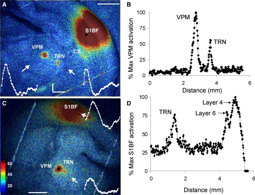
Demonstration of corticothalamic and thalamocortical activation in the mouse somatosensory slice. A: Fourier image demonstrating VPM, TRN, and cortical supragranular activation after electrical stimulation of the infragranular layers of S1BF. FA, flavoprotein autofluorescence; ROI, region of interest; S1BF, primary somatosensory cortex-barrel field; TRN, thalamic reticular nucleus; VPM, ventral posterior nucleus of thalamus. Black circle represents stimulus site. White insets demonstrate time courses of activation in 3 × 3-pixel ROIs corresponding to white arrows. Horizontal scale bar = 1 mm. Right-angle scale bar is for time course data. Abscissa = 5 s; ordinate = 1% increase in FA. B: response amplitude (expressed as percentage of peak of VPM spectral power at the stimulus frequency) vs. spatial location along an imaginary horizontal line passing through VPM and TRN. Stimulus parameters: 50 μA, 20 Hz, 10-ms pulses, train duration = 1 s with 14-s intertrain interval × 5-pulse train. C: Fourier image in a different slice demonstrating activation of TRN and S1BF after electrical stimulation of VPM. Black circle represents stimulus site. White insets demonstrate time courses of activation of ROIs corresponding to white arrows. Scales of time courses correspond to right-angle scale bar in A. Horizontal scale bar = 1 mm. D: response amplitude (expressed as percentage of peak of TRN spectral response) vs. spatial location along an imaginary line connecting TRN and the activation focus in S1BF. Stimuli in D–F were monopolar electrical stimulations at 50 μA, 2-ms-duration pulses, 20 pulses/s for 1-s train, 14-s intertrain intervals for a total of 2 pulse trains, and 28 s of imaging time.

Image processing

All activation images were generated in Matlab and all anatomic images were in TIFF format and were imported into CorelDraw for final preparation. Anatomic images in Figs. 10 and 11 were contrast-stretched in Photoshop to enhance anatomic boundaries.

RESULTS

Electrical stimulation studies

The goals for the first sets of experiments were to 1) determine the ability of FA to detect long-range neural connections in vitro, 2) determine the spatial and temporal resolution of FA signals, and 3) determine the sensitivity of FA to detect neural activity. For these experiments, we characterized FA responses to electrical stimulation in mouse somatosensory thalamocortical slices. Monopolar electrical stimulation in the infragranular layers of S1BF produced activation in layers 2/3 of the overlying cortex and produced small foci of activation in the VPM and TRN nuclei of the thalamus (Fig. 2A). Insets in Fig. 2A illustrate the relatively protracted and biphasic time courses of activation in VPM and TRN. Figure 2B demonstrates the average response amplitude versus slice location computed using a 10-pixel-wide rectangular box aligned and centered along an imaginary line passing through VPM and the TRN. The resultant function was used to compute the width at half-maximum amplitudes for the VPM and TRN, which were 280 and 100 μm, respectively. In three separate experiments, cortical stimulation produced foci of activation in the VPM with widths at half-maximum of 160 μm each time; in an additional experiment where TRN activation was observed, the half-width was 120 μm (data not shown). These data suggest that the greatest experimentally determined spatial resolution is in the range of 100–200 μm. It should be noted that this half-width is a conservative estimate of spatial resolution since the width represents a combination of both the optical resolution (limited by light scattering) and the finite size of the neuronal population activated (that is, the activated area is larger than a theoretical point source).

We also found that stimulation of VPM robustly activated S1BF and often activated TRN in the thalamocortical slice, as demonstrated in Fig. 2, C and D. Insets in Fig. 2C illustrate the characteristic protracted and biphasic time course of activation in the TRN and S1BF. Figure 2D illustrates the spatial dimension of activation of the TRN and layers 4 and 6 of S1BF. We have found that we can reliably elicit somatosensory thalamocortical activation in at least one to two slices per animal.

We examined the spatiotemporal properties of FA across multiple somatosensory cortical regions after picospritzer application of glutamate into the VPM (Fig. 3). Figure 3A is an expanded view of the somatosensory cortex under fluorescence illumination, illustrating the S1BF (identified by the regular patterns of barrels), the S1-trunk region, and S2. Analysis of the time course of activation in the cortex using Δf/f images revealed a peak of activation in S1BF at around 3 s after stimulation of VPM, followed by peaks at about 5.5 s in both S1-trunk area and S2 (Fig. 3, B and C). The time courses of activation in ROIs in these three cortical structures revealed a latency lag of about 2 s for both S1-trunk and S2, compared with S1BF (Fig. 3D), which suggests that S1-trunk and S2 are activated polysynaptically, potentially through interareal corticocortical projections (Staiger et al. 1999; Zhang and Deschênes 1997). This analysis in the temporal structure of the response also permits examination of underlying spatial heterogeneities, such as the border between S1BF and S2. This border is evident in the phase image, shown in Fig. 3E, but is not apparent in any individual Δf/f image. This transition is made clear in Fig. 3F, where the percentage of activated pixels with response lag of <4.5 s (blue) is compared with the percentage of pixels with response lag >4.5 s (red). There is an abrupt transition between these two, which corresponds nearly exactly to the transition from S1BF to S2, determined by the transition from barrels (periodicity in the layer 4 intensity of the baseline image) to tissue without barrels (no periodicity in intensity; black line). Note that the temporal discontinuity occurred only at physiological borders and that the FA latency was similar throughout S1BF, despite the high likelihood that a significant proportion of the S1BF activation is polysynaptic.

FIG. 3.

Illustration of spatiotemporal pattern of the FA response in cortex after focal stimulation of VPM with 2 mM l-glutamate. A: expanded view of a baseline fluorescence imaging demonstrating the borders (dotted lines) of S1-trunk area (S1-Tr), S1BF, and S2, based on the presence of barrels in S1BF. Scale bar = 1 mm. B: Δf/f image of FA activation in S1BF after thalamic stimulation taken at 3.0 s after stimulus onset. C: Δf/f image of FA activation in S1BF after thalamic stimulation taken at 5.5 s after stimulus onset. D: time courses of activation in an ROI over the S1BF (purple), S1-Tr (green), and S2 (red) using a 1-s-long window for moving average. E: temporal phase of responses, illustrating phase lag of about 2 s in S1-Tr and S2 part of the cortex, and a relatively sharp demarcation of the S1BF/S2 border based on phase differences. See methods for details regarding phase analysis; only pixels with response amplitude >1% above baseline are shown. Pseudocolor scale bar represents phase lag in seconds. Horizontal scale bar = 1 mm. F: plot of percentage of the maximum number of pixels activated in a 30-pixel box scrolled along the diagonal line shown in E, for pixels with a lag of <4.5 s (purple) and lag >4.5 s (red). Overlaid in black is a high-pass filtered plot of pixel intensity of baseline fluorescence image, demonstrating regularity over the first 0.5 mm, corresponding to the barrel field, then transitioning to nonperiodic signal in S2 for both figures. G: time course of activation at the thalamic stimulation site (blue) and in a series of 40 pixels taken from a ring surrounding the thalamic stimulation site (green), normalized to the peak from the stimulation site. Inset shows areas in the center of the stimulus site (blue) and surrounding the site (green) from which pixels were derived for this analysis. l-Glutamate was applied through a picospritzer with pressure pulses (1 psi) 8 ms in duration, applied at 20 pulses/s, with 1-s train duration, with 14-s intertrain interval. Scale bar = 1 mm.

It is possible that the activation of S1-trunk and/or S2 was related to the spread of glutamate to adjacent thalamic areas. However, as illustrated in Fig. 3G, comparison of the time course and amplitude of activation of an ROI within the stimulus site, and from 40 pixels taken from the directly adjacent ring, did not demonstrate significant activation adjacent to the stimulus site. Furthermore, we have consistently seen similar increases in latency in S2 after direct glutamate-based stimulation of S1BF (Theyel et al. 2008), also suggesting that diffusion of glutamate in the thalamus is not likely responsible for the latency increase. The spatiotemporal structure of responses can therefore be used to infer the gross order of activation within a large thalamocortical circuit. For illustration of this experiment in real time, see Supplemental Movie S2.

To determine the sensitivity of FA to detect long-range neural activity, we used two complementary experimental paradigms: 1) thalamocortical activation using a single stimulus amplitude, while recording postsynaptic activity in cells within and outside of the cortical FA activation zone; and 2) thalamocortical activation using a range of stimulus amplitudes to compare thresholds of postsynaptic activity and FA activation. Recording of loci was determined via visual guidance since barrels were easily visualized in the living slice (see Fig. 3A). All recordings were from neurons in the middle cortical layers of the S1BF during VPM stimulation. Figure 4, A–C demonstrates typical FA activation maps and time courses in S1BF, with example current-clamp recordings from neurons located in (blue) and out (red) of the FA activation zones shown in Fig. 4B. Both optical and electrical activations were measured in response to thalamic stimulation at 20 μA above FA activation threshold and identical stimuli were used to generate the FA and synaptic responses. We recorded from 13 S1BF neurons in three slices within the activation zones (defined as having an increase in fluorescence of >1%, relative to baseline) and from 9 neurons outside of the activation zone. We found that 12/13 of the neurons within the activation zone were depolarized by ≥2 mV in response to electrical stimulation of the thalamus (1/13 showed no response), whereas none of the 9 neurons outside of the FA response area [mean distance from edge of activation zone containing pixels with >1% increase in FA = 389 ± 269 (SD) μm] responded with depolarizations of >2 mV. We chose 2 mV as the criterion for electrical responsiveness because the average SD of the resting membrane potential for all 22 cells ranged from 0.4 to 1.34 mV, mean = 0.73 ± 0.77 (SD) mV (see Supplemental Fig. S2 for distribution of SDs). The range of first excitatory postsynaptic potential (EPSP) latencies, relative to the first pulse in the train, was 5.0 to 81 ms; 6/12 of these neurons had latencies of <10 ms and a mean latency of 6.4 ± 0.58 ms with average jitter of 320 μs, suggesting that they were monosynaptically activated. The remaining neurons had a mean latency of 27.9 ± 27.9 ms, suggesting that they were polysynaptic or evoked by later pulses in the train. Figure 4D summarizes the relationship between FA and EPSP amplitude (note that EPSP amplitude measurements are from different neurons). Blue symbols correspond to cells within the FA activation zone and red symbols correspond to cells outside of the activation zone. Triangles represent short-latency, low-jitter (presumably monosynaptic) responses. These data suggest that in a region adjacent to an FA activation zone, FA signal amplitude of <1% above baseline predicts the absence of synaptic activation. Note that this roughly corresponds to twice the mean SD of the FA signal of the 9 ROIs outside the activation zone (0.42 ± 0.17%). In addition, we recorded from 16 neurons in the LGN after electrical stimulation of the OT. We found that all 10 neurons in the FA activation zone exhibited EPSPs in response to OT stimulation, and none of the 6 neurons outside the FA activation zone (mean distance from edge of >1% FA activation zone = 232 ± 52 μm) did so. We measured EPSP latency in 5/7 LGN neurons (2 neurons had EPSP onsets <2 ms and therefore temporally overlapped the stimulus artifact). Of the 5 remaining neurons, mean EPSP latency was 3.73 ± 1.54 ms with mean jitter of 290 μs (range 80–480 μs), suggesting that these responses were monosynaptic. Based on recordings in both areas the optically defined activation zone is thus generally coextensive with the area in which neurons are depolarized.

FIG. 4.

Comparison of FA response in S1BF to synaptic responses in neurons recorded via whole cell patch clamp. A: increase in autofluorescence in S1BF after electrical stimulation of VPM (scale bar = 1 mm). B: example voltage traces (5 traces each, overlaid) for a cell in the FA activation zone (blue) and another cell outside the FA activation zone (red). Vertical lines are stimulus artifacts. C: change in fluorescence relative to baseline in 2 × 2-pixel ROI either in the FA activation zone (blue) or outside of the zone (red). D: scatterplot of FA amplitude (expressed as percentage increase from baseline, abscissa) and corresponding excitatory postsynaptic potential (EPSP) amplitude (ordinate). Red symbols represent cells that were not in the FA activation zone. Blue symbols represent cells that were in the FA activation zone. Blue triangles correspond to cells in the FA activation zone that were likely monosynaptically activated based on short EPSP latency. Stimulus parameters: monopolar electrical stimulation using 2-ms-duration pulses, 40 pulses/s for 100-ms train, 14-s intertrain intervals for a total of 2 pulse trains, and 28 s of imaging time.

To study the relationship between FA and EPSP amplitude, we recorded polysynaptic activity from neurons in a region that showed increases in FA but that was outside the peak FA activation zone and, presumably, outside of the direct thalamocortical synaptic input zone. Polysynaptic responses were measured to maximize the dynamic range of electrical currents, which is typically narrow for individual neurons within the monosynaptic thalamic input zone (Gil et al. 1999). We measured changes in FA in response to a wide range of stimulation currents and measured postsynaptic responses to the same set of currents. The example in Fig. 5A illustrates the FA response in S1BF to three different amplitudes of stimulation in the VPM and the corresponding synaptic current traces (voltage clamp near the GABA_A reversal potential of −60 mV) for a layer 4 cell, whose location is marked with a red circle. We recorded from four cells in this slice and observed synaptic latencies in the range of 500–1,000 ms, consistent with polysynaptic activation of S1BF after thalamic stimulation (Agmon et al. 1996). As shown, no FA or synaptic response was seen with a 10-μA stimulus amplitude and there was a progressive increase in both FA (Fig. 5A) and inward charge transfer (Fig. 5B) with increasing stimulus amplitude. Input–output curves were generated for the four neurons in layer 4 of a cortical FA activation zone in a single slice. The FA output was defined as the percentage change in a 3 × 3-pixel box around the recorded cell. The average data ± SE and Naka–Rushton functions for the data are shown in Fig. 5C. The half-maximum stimulus currents from the Naka–Rushton fits were 23.2 μA for FA and 21.4 μA for the recorded inward charge transfer. The slopes were 0.41 and 0.66%/μA⁻¹ for FA and inward current, respectively. We compared the FA response and total inward charge transfer across five stimulus amplitudes for the four neurons recorded in this portion of the study. The scatterplot, shown in Fig. 5D, demonstrates a statistically significant correlation between FA amplitude and inward charge transfer (R² = 0.67, P < 0.001, t = 6.02, correlation function y = 5.0x − 1.6). These data suggest that the dynamic range for thalamocortical activation measured by FA in this slice is from 1 to 3% increase in FA from baseline. Further, these data are consistent with those in Fig. 4 that show an absence of underlying synaptic activity when the FA increases by <1%.

FIG. 5.

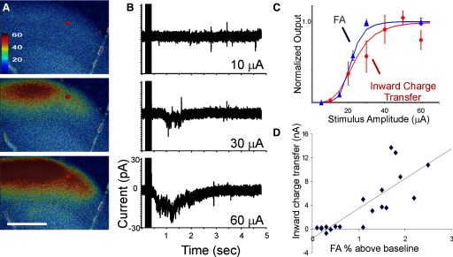
A: FA in somatosensory cortex in response to VPM stimulation at 10, 30, and 60 μA. B: current changes in a cell at the location of the red spot held in voltage clamp at −60 mV. The traces represent the mean of 10 runs. Vertical lines on the left of the traces represent the stimulus artifact. C: normalized mean input–output functions from 4 cells (inward charge transfer, red) and their corresponding ROIs (increase in fluorescence in 3 × 3-pixel areas around cell, blue). Fitted function is a Naka–Rushton function (see methods) and error bars represent normalized SE. D: scatterplot of FA amplitude (expressed as percentage increase from baseline) vs. total inward charge transfer for all stimulus amplitudes across 4 neurons. R² = 0.67, t = 0.001, t = 6.02, linear fit: y = 5.0x − 1.6. Stimulus parameters: monopolar electrical stimulation using 2-ms-duration pulses, 40 pulses/s for 250-ms train, 14-s intertrain intervals for a total of 2 pulse trains, and 28 s of imaging time.

To determine whether the FA response was dominated by either presynaptic or postsynaptic activity, we exposed tissue slices to bath-applied ionotropic glutamate blockade (50 μM DNQX + 100 μM AP5). Figure 6A demonstrates the FA response in S1BF after 30 μA electrical stimulation in VPM. Figure 6B demonstrates that the response in S1BF as well as most of the local thalamic response was eliminated after incubation of the tissue with ionotropic glutamate receptor blockers. Despite increasing the electrical stimulus strength fourfold to 120 μA, no signal was seen in S1BF (Fig. 6C), though there was an increase in activation around the stimulus site, suggesting adequate thalamic stimulation was achieved. The cortical response returned after a 20-min wash period (Fig. 6D). Similar results were seen in the OT-to-LGN preparation (data not shown). These data suggest that the bulk of the FA response is postsynaptic in origin.

FIG. 6.

Blockade of ionotropic glutamate receptors eliminates the bulk of the thalamocortical FA response. A: electrical stimulation (30 μA) in VPM generates a strong response in the S1BF in normal ACSF. B: after 15-min incubation with ionotropic glutamate blockers (50 μΜ DNQX + 100 μM AP5), the cortical response was nearly eliminated. C: increasing the stimulus amplitude to 120 μA did not produce a cortical response. D: after 20-min washing in normal ACSF, the cortical response recovered. All images are overlaid Fourier images. Stimulus parameters: monopolar electrical stimulation using 1-ms-duration pulses, 40 pulses/s for 1,000-ms train, 14-s intertrain intervals for a total of 2 pulse trains, and 28 s of imaging time. Scale bar = 1 mm. ACSF, artificial cerebrospinal fluid; AP5, d-2-amino-5-phosphonovaleric acid; DNQX, 6,7-dinitroquinoxaline-2,3-dione.

Photostimulation studies

Figure 7 illustrates five examples of FA activation after laser photostimulation using trains of five pulses at 20 pulses/s, individual pulse duration of 10 ms, and pulse amplitude of 35 mW. In Fig. 7, A and B, corticocortical activation is seen from layer 2/3 of S1BF to S2 and from layer 5 of V1 to V2, respectively. Although V1 is known to have multiple local targets, most are not captured in the coronal plane (Wang and Burkhalter 2007), suggesting why a single projection was seen. In Fig. 7C, thalamocortical activation is seen from VPM to S1BF. Figure 7D demonstrates activation of the auditory cortex after stimulation of the medial geniculate body, as well as a previously undescribed auditory thalamostriatal projection in the auditory thalamocortical slice. Diffuse corticocortical, corticostriatal, and corticothalamic activations are seen after laser stimulation of the infragranular layers of S1BF in Fig. 7E. Note that in Fig. 7E, the maximum power of the laser (67 mW) was required to achieve thalamic activation, resulting in widespread cortical activation, where the connectivity is likely the strongest. In all cases, remote activation was eliminated when the tissue was bathed in a medium containing 0 mM CaCl₂ and 4 mM MgCl₂ (third column, “synaptic blockade”) and returned after washout (right column). Note that activations in all of these pathways using photostimulation with FA have been reproduced in slices from additional animals.

FIG. 7.

Examples of long-range FA activation using photostimulation. Left column shows baseline fluorescence images (stimulation wavelength 450–490 nm; emission wavelength >515 nm). All color images represent the Δf/f at each pixel, for single trials (A–D) or 5 trials (E) with no spatial smoothing. The data for the 2nd column were obtained in normal ACSF; the 3rd column in “synaptic blockade” ACSF, which contains 0 mM Ca²⁺ and 4 mM Mg²⁺; and data for the 4th column were collected in normal ACSF after a 15-min wash period. White lines going across the images are the strings used to hold down the slices. A: stimulation in layer 2/3 of S1BF, with activation in S2. B: stimulation in layers 5 and 6 of V1, with response in V2. C: stimulation in VPM with activation in S1BF. D: stimulation in the MGB, with activation in TRN, CS, A1, and AAF. E: stimulation in layers 5 and 6 of S1BF with activation of S1, CS, TRN, and VPM. Scale bar in all cases = 1 mm. Stimuli consisted of trains of 5 laser pulses, presented at 20 pulses/s, with pulse durations of 10 ms. Laser power = 35 mW, except in E, where laser power was 67 mW. All images are single runs, without averaging, with the exception of E, where 5 runs were averaged. Color bar illustrates the pseudocolor scale corresponding to values of % FA increase. A1, primary auditory cortex; AAF, anterior auditory field; CS, central sulcus; MGB, medial geniculate body; V1, primary visual cortex; V2, secondary visual cortex.

We determined the minimum duration and amplitude of laser pulses required to elicit a thalamocortical response. Not to confound amplitude and duration contributions to S1BF responses, for investigations of pulse-duration effects, pulse amplitude was held at a value consistently found to generate strong responses (67 mW). Similarly, for amplitude titrations, pulse width was held at a high value (10 ms).

Figure 8, A–E shows examples of the effect of increasing pulse duration on thalamocortical FA responses. At pulse durations of ≤0.5 ms, no cortical response is observed. At a pulse duration of 0.53 ms, a prominent response is seen in layers 2–4 and 6 of the S1BF. At longer pulse durations, no further increase in response amplitude was observed. This experiment was performed in two animals and the composite data are shown in Fig. 8F. The blue diamonds correspond to the signal from the S1BF and red diamonds are from the stimulus site in the VPM. Note that although there appears to be a very sharp threshold for driving cortical fluorescence (0.5- to 0.6-ms duration), there is a gradual increase in FA at the stimulus site with increasing stimulus duration.

FIG. 8.

A–E: Δf/f overlay images, all done as single trials, demonstrating the effect of increasing pulse duration in VPM on FA responses in S1BF. No response is seen at stimulus durations of ≤0.5 ms, whereas prominent S1BF responses are seen at stimulus amplitudes >0.53 ms. F: composite data from 2 animals. Ordinate represents the percentage of maximum Δf/f value for all S1BF responses (blue diamonds) or VPM responses (red diamonds), respectively. Arrow corresponds to stimulus site. Scale bar = 1 mm.

We also determined the minimum amplitude of a short train of pulses required to elicit a thalamocortical FA response. Figure 9, A–E shows examples of the effect of increasing amplitude (pulse-train parameters: five pulses, pulses 10 ms in duration presented at 20 pulses/s). At laser powers of 4 and 5 mW, no response is seen in the central portion of S1BF. At amplitudes of ≥6 mW, a response is seen in layers 2–4 and 6 of S1BF. There is no apparent increase in signal amplitude over the center of S1BF, although the signal area spreads laterally within S1BF as the stimulus power increases. This experiment was performed at several amplitudes in two animals and the composite data are shown in Fig. 9F. There appears to be a sharp transition in the S1BF at about 7–8 mW. Above this stimulus amplitude, there is no increase in cortical FA response. In contrast, stimulus amplitudes <36 mW do not elicit a measurable response in VPM, but elicit a strong response at 36 mW.

FIG. 9.

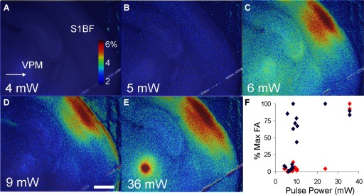
A–E: Δf/f overlay images, all done as single trials, demonstrating the effect of increasing pulse amplitude in VPM on FA responses in S1BF. Stimuli consisted of pulse trains, containing 5 pulses, 10-ms pulse duration, 40-ms interpulse interval. No response is seen at stimulus intensities of ≤5 mW, whereas prominent S1BF responses are seen at stimulus amplitudes >5 mW. F: composite data from 2 animals. Ordinate represents the percentage of maximum Δf/f value for all S1BF responses (blue diamonds) or all VPM responses (red diamonds), respectively. Arrow corresponds to stimulus site. Scale bar = 1 mm.

These, and the monotonically increase in VPM activation with stimulus strength in Figs. 8F and 9F, suggest that the saturating responses seen in S1BF are not an artifact of saturation of VPM activation.

Mapping the topography of projections from VPM to cortex and VPM to TRN can readily be performed with photostimulation combined with FA. Figure 10, A–C shows the cortical response to progressive ventral movement of the photostimulation site in VPM following near-threshold activation, which was used to achieve a narrow area of activation in the cortex. The relatively low signal-to-noise ratio in these studies can be attributed to the low stimulation amplitudes used. Figure 10D demonstrates the topography of the thalamocortical projection: the centroid of the cortical activation zone moved progressively ventrally, tracking with the stimulation sites in VPM.

FIG. 10.

Mapping of projections from VPM to S1BF using laser uncaging of glutamate and FA. A–C: Δf/f overlay images illustrating the sequential movement of the laser stimulation site to progressively more ventral portions of VPM. D: composite image of the stimulation sites and the centroid of the response sites from A (blue), B (red), and C (yellow). Stimulus parameters: 5 pulses, duration = 10 ms, interpulse interval = 40 ms, pulse amplitude = 8 mW. All scale bars = 1 mm.

Figure 11, A and B demonstrates representative examples of focal activation in two sites of TRN after photostimulation in two sites of VPM and a summary image illustrating all six photostimulation sites and six response sites is shown in Fig. 11C. The relationship between the location of the stimulus site, relative to its ventromedial border, and the response site in the TRN, relative to its ventromedial border, is shown in Fig. 11D. The relationship was linear with a correlation coefficient of 0.995, t-value = 28.3, P < 0.00001, and null hypothesis of slope = 0. It is important to note, in support of the high degree of practicality of this technique, that this map was generated in a single run lasting about 30 s. The spatial resolution of this map, as determined using the full-width at half-maximum height of the TRN activation zones, is 223 ± 29 μm (n = 6 TRN sites). The real-time video from this experiment is shown in Supplemental Movie S1.

FIG. 11.

Mapping of projections from VPM to TRN using laser uncaging of glutamate and FA. A and B: Δf/f overlay images illustrating stimulus sites in VPM and response sites in TRN in the same slice. C: summary image of VPM and TRN illustrating multiple laser stimulation sites in VPM and their corresponding response outlines measured at 90% of the peak response in the TRN. Scale bar = 1 mm. D: location of stimulation site relative to the medioventral border of the VPM vs. location of response site in TRN relative to the medioventral border of the TRN. Colors of points correspond to the stimulus–response pairs seen in C (regression line: y = 0.92x + 57.4E). Scatterplot illustrating VPM stimulus site vs. TRN response site across 4 animals. Each color corresponds to a different animal. Stimulus parameters: 20 pulses, duration = 10 ms, interpulse interval = 40 ms, pulse amplitude = 67 mW. F: comparison of VPM–TRN mapping coordinates using 3 different stimulus paradigms. Blue diamonds and regression line (y = 0.83x + 102) represent data obtained using 5-s interstimulus intervals, applied sequentially from the dorsolateral border systematically toward the ventromedial border of VPM. Red diamonds and regression line (y = 0.85x + 95) represent data obtained in a similar fashion as above, but at 14-s interstimulus intervals. Green diamonds and regression line (y = 0.91x + 0.3) represent VPM–TRN mapping obtained using 5-s interstimulus intervals, with pseudorandomly ordered stimulation sites throughout the VPM.

Maps of the projection from VPM to TRN were repeated in slices from three more animals, with nearly identical results. A summary of stimulus–response pairs across all three animals is found in Fig. 11E. In one of these animals we compared maps generated under three conditions: 1) a map with 5-s intervals with pseudorandom selection of stimulation points in the VPM, 2) a map generated with systematic movement of stimulation site across the VPM, with 5-s interstimulus intervals, and 3) a map generated with systematic movement of stimulation site across the VPM, with 14-s interstimulus intervals. We found nearly identical maps under all three conditions (see Fig. 11F), which suggests that there is no interaction between stimulus and response pairings using a 5-s interstimulus interval.

DISCUSSION

We have shown that 1) FA is a sensitive marker for long-distance synaptic activation in vitro with spatial resolution of ≥100–200 μm, 2) the source of the thalamocortical FA signal in slice is primarily postsynaptic, and 3) FA coupled with photostimulation provides a rapid tool to explore novel circuitry and map neural projections in vitro. This technology represents a significant advance over previous approaches because it avoids the use of fluorophore-loading procedures and, being all-optical, allows rapid interrogation of slices to reveal their underlying neural circuitry.

FA signal characteristics

We observed FA signal amplitudes that are comparable to those reported by other investigators in vitro (Shibuki et al. 2003) and slightly greater than that previously observed in vivo (Husson et al. 2007; Reinert et al. 2004; Shibuki et al. 2003). Although the current study did not investigate the mechanism of FA signal generation, the current data add to previous work suggesting that both short-range and long-range FA signals are not dependent on intrinsic hemodynamic signaling (Husson et al. 2007; Shibuki et al. 2003), since blood is absent from the preparation. The time course of activation, with a peak response within 1–3 s after stimulus onset and protracted downward slope followed by a tendency for the optical signal to decrease below its baseline value, is very similar to descriptions by other investigators using FA (Husson et al. 2007; Reinert et al. 2004; Shibuki et al. 2003). The underlying nature of the late negative-going wave is not known, although its partially selective elimination by the glial toxin fluoroacetate suggests that this portion of the waveform is derived from glial glutamate transport (Reinert et al. 2007).

Our data suggest that the source of the FA signal after thalamocortical stimulation is primarily postsynaptic and triggered by the activation of ionotropic glutamate receptors. At very high electrical stimulus amplitudes, the residual signal observed in VPM (Fig. 6C) suggests that it is possible to visualize somatic (nonsynaptic) activation with high stimulus amplitudes. Similar experiments in other systems have had mixed results. Corticocortical FA activation in vitro and inferior olive–to–cerebellar cortex activation in vivo were eliminated after ionotropic glutamate blockade (Dunbar et al. 2004; Hishida et al. 2007). In contrast, FA activation after local cortical stimulation was only partially blocked by this manipulation (Dunbar et al. 2004; Shibuki et al. 2003). The source of the residual FA signal in this case is not known, although local electrical stimulation of cortex may engage nonglutamatergic systems such as monaminergic fibers. The present study does not allow us to distinguish between postsynaptic subthreshold and spiking activity as a source of the cortical signal; further work will be needed to clarify this.

Sensitivity, spatiotemporal resolution, and inferences about network activity

One important factor that will influence the utility of this technique is the likelihood that a given area of FA activation represents underlying synaptic activity. We found that the sensitivity of FA in vitro is comparable with that of both mono- and polysynaptic activation, measured via whole cell patch clamp. This conclusion is based on the nearly 100% correspondence between the presence of synaptic responses and the optical activity in the target region (Fig. 4) and on the virtually indistinguishable thresholds for synaptic and FA activation (Fig. 5). These data suggest that regions in which FA activation is <1% above baseline, even adjacent to activation zones, have little synaptic activity.

An additional important factor for the utility of FA is its potential capacity to assist in the study of network activity, which depends on both the sensitivity and spatial resolution of the imaging technique. We estimate the spatial resolution of FA to be around 100–200 μm, based on the smallest width at half-maximal amplitudes observed in VPM and TRN (Fig. 2B). This estimate is a conservative one, since the most appropriate tool to assess spatial resolution is a point source and the thalamic activation is presumably larger than this. It should be noted that the spatial breadth of activation that we observed was varied in relation to the known underlying synaptic organization of the activated structures. For example, areas with relatively sparse intrinsic interconnectivity (e.g., dorsal thalamus, TRN) tended to demonstrate relatively focal activation. In contrast, areas with dense neuronal interconnectivity (e.g., the cortex) tended to have a broad area of FA signal, even when near-threshold stimuli are used (compare cortical vs. subcortical activation in Fig. 2, B and D). Nevertheless, using a simple centroid calculation, we were able to quickly generate a thalamocortical map that replicates previously published maps. Additionally, by using calcium imaging in the thalamocortical slice and using an experimental paradigm similar to that in the current study, cortical activations were produced that had a characteristic breadth similar to that currently shown (Beierlein et al. 2002). It was proposed that this breadth was likely due to rapid spread of neuronal signal throughout the S1BC. Such rapid spread would be time-collapsed with FA. It is also important to contrast the mode of cortical activation in the current study (focal stimulation of thalamus) with sensory stimulation, since sensory stimulation can focally activate the cortex to generate precise maps (Friedman et al. 2004; Weliky et al. 1996). It may be that sensory stimulation—by engaging a range of loci within the thalamus—permits sharper cortical activation via lateral inhibitory interactions, which would not be seen in our stimulus paradigm, but, incidentally, would be highly amenable to study using FA.

The degree of spatial resolution described earlier coupled with the high sensitivity of FA for mono- and polysynaptic activation suggest that all activated elements in an intact and adequately stimulated neural network can be visualized in vitro using FA. As such, this technique has a high utility for rapidly identifying all nodes of a neuronal network prior to engaging in their systematic study. Refinements to this technique, such as the use of higher-sensitivity recording equipment (e.g., electron-multiplying charge-coupled device) or manipulations of bathing media to limit synaptic transmission, may ultimately allow the investigation of monosynaptic projections. When studying a polysynaptic network, the relatively protracted time course of activation generally limits the use of temporal order of activation to infer the direction of signal flow within a network. One notable exception was in the temporal relationship of activation between S1BF and its known targets: the S1-trunk and S2 areas (Staiger et al. 1999; Zhang and Deschênes 1997). We found a sharp increase in the phase lag of the FA signal of about 2 s in the secondary cortical regions. This is consistent with the finding that propagating waves are delayed at areal boundaries (Xu et al. 2007) and event-related functional magnetic resonance imaging (fMRI) studies in which timing differences on the order of seconds within distributed networks have been found (Kraut et al. 2003). These data lead to several open questions: 1) How do millisecond-level differences in latency manifest as second-level differences in FA? 2) Are the differences in phase purely related to synaptic latency or are there other factors, such as intrinsic differences in the temporal properties of neurometabolic coupling in different brain regions or the recruitment of slower (e.g., metabotropic) responses in S2 versus S1BF? Answers to these questions will not only further our understanding of the underlying biology but will also inform efforts to use temporal structure in other forms of metabolic imaging, such as blood oxygen level–dependent based fMRI (Kraut et al. 2003).

Flavoprotein autofluorescence for mapping

We found that robust thalamocortical responses were elicitable in single trials using stimulus amplitudes as low as approximately 6 mW (in a train of five pulses, each of 10-ms duration; Fig. 8), and that stimulus amplitudes as high as 67 mW can be used for multiple runs without rundown of the response (Fig. 7E), suggesting a lack of phototoxicity or rundown in this range of stimulus parameters. This is particularly notable since trains of pulses were used in these experiments that have the potential to cause glutamate-receptor desensitization or local glutamate depletion. We have not systematically compared the responses to trains of pulses to individual pulses, but have observed strong responses with single pulses. For example, we found that, using single pulses, durations as low as 0.5 ms (at stimulus amplitude of 67 mW) elicited robust responses in S1BF. Interestingly, thalamocortical activation in the peak of the cortical activation zone appeared to have an all-or-none character, which is consistent with what was previously seen in recordings from layer 4 neurons in vitro (Gil et al. 1999). The nonlinear nature of the responses seen in S1BF is unlikely to be an artifact of saturating responses in VPM since VPM activation monotonically increased with increased stimulus power or duration (Figs. 8F and 9F). These data suggest that the all-or-none response seen in S1BF is created in the cortex.

We confirmed the previously established topographic relationship between VPM and S1BF such that the dorsolateral portions of VPM project to the medial portions of S1BF and that progressively ventromedial stimulation sites in VPM activate progressively lateral locations in S1BF. This organization has been shown before via tracer injection into several different animals (Dawson and Killackey 1985) and in the slice using electrical stimulation and recording (Agmon and Connors 1991). Our approach has many advantages over these methods. Compared with tracer studies, photostimulation with FA permits mapping in a single animal. This is of great consequence because it is often necessary to assess the impact of a behavioral or pharmacological manipulation on the topography of neural circuitry; moreover, the ability to use single animals for mapping significantly reduces variability in the resulting maps. Traditional approaches, such as electrical stimulation and recording, are limited because of the inability to assess the spread of activation at either the stimulus or the response site. In contrast, with photostimulation and FA, one can clearly assess the spread of activity in both sites. In addition, our approach carries no assumptions about the underlying connectivity since one can image at low magnification (×2.5) and observe the response anywhere in the slice. Further, the use of photostimulation ensures that one is studying orthrodromic projections, since both electrical stimulation and dye injection are compromised by the potential to stimulate or label fibers of passage, respectively. Finally, our approach allows the rapid construction of maps (on the order of minutes).

The connectivity pattern between VPM and TRN has been suspected from the somatotopic maps in the two structures (Shosaku et al. 1984), but has not been directly mapped. We used photostimulation plus FA to map the projection from VPM to the TRN and found a clear dorsoventral gradient in the projections (see Fig. 9). This map was reproducible in other animals and was obtained in about 30 s. This map (and the ability to rapidly generate it in a viable slice) will allow us to ask more sophisticated questions about the mapping of dorsal thalamus to TRN. Some of these include studying the fidelity of mapping between the first-order (VPM) versus the higher-order (posterior medial division) somatosensory thalamus to the TRN or translating cross-whisker, or cross-modal, inhibition, previously described in dorsal thalamus–TRN networks at the individual-cell level (Crabtree and Isaac 2002; Desilets-Roy et al. 2002; Kimura 2007), to systematic maps of cross-whisker or cross-modality interaction.

Conclusions

We have demonstrated that photostimulation with FA is a sensitive, rapid, and relatively easily implemented method for mapping long-range neural circuits in vitro. Although another form of “hands-free” stimulation and imaging in slices has recently been developed (Nikolenko et al. 2007), it requires cellular loading of a fluorophore and is suitable only for short-range connections, rather than the long-range connections seen here. In addition, our ability to conduct FA experiments in multiple systems (visual, auditory, and somatosensory) and at multiple levels (VPM to TRN, thalamus to cortex, cortex to thalamus and basal ganglia, cortex to cortex) suggests that this technique will be transferable to the experimental needs of the broader neuroscience community. Finally, since this technique uses few assumptions about the presence of neural circuitry in a slice, we anticipate that it has the potential to reveal the presence of unexpected circuitry that can prompt new lines of investigation.

GRANTS

This work was supported by the United States Public Health Service; National Institutes of Health Grants DC-008320 to D. A. Llano, EY-03038 and DC-008794 to S. M. Sherman, and GM-07281 to A. K. Mallik; and a Mallinckrodt and Brain Research Foundations grant to N. P. Issa.

REFERENCES

- Agmon and Connors 1991.Agmon A, Connors BW. Thalamocortical responses of mouse somatosensory (barrel) cortex in vitro. Neuroscience 41: 365–379, 1991. [DOI] [PubMed] [Google Scholar]
- Agmon et al. 1996.Agmon A, Hollrigel G, O'Dowd DK. Functional GABAergic synaptic connection in neonatal mouse barrel cortex. J Neurosci 16: 4684–4695, 1996. [DOI] [PMC free article] [PubMed] [Google Scholar]
- Beierlein et al. 2002.Beierlein M, Fall CP, Rinzel J, Yuste R. Thalamocortical bursts trigger recurrent activity in neocortical networks: layer 4 as a frequency-dependent gate. J Neurosci 22: 9885–9894, 2002. [DOI] [PMC free article] [PubMed] [Google Scholar]
- Catalano and Shatz 1998.Catalano SM, Shatz CJ. Activity-dependent cortical target selection by thalamic axons. Science 281: 559–562, 1998. [DOI] [PubMed] [Google Scholar]
- Cohen 1973.Cohen PJ Effect of anesthetics on mitochondrial function. Anesthesiology 39: 153–164, 1973. [DOI] [PubMed] [Google Scholar]
- Crabtree and Isaac 2002.Crabtree JW, Isaac JTR. New intrathalamic pathways allowing modality-related and cross-modality switching in the dorsal thalamus. J Neurosci 22: 8754–8761, 2002. [DOI] [PMC free article] [PubMed] [Google Scholar]
- Cruikshank et al. 2002.Cruikshank SJ, Rose HJ, Metherate R. Auditory thalamocortical synaptic transmission in vitro. J Neurophysiol 87: 361–384, 2002. [DOI] [PubMed] [Google Scholar]
- Dawson and Killackey 1985.Dawson D, Killackey H. Distinguishing topography and somatotopy in the thalamocortical projections of the developing rat. Brain Res 349: 309–313, 1985. [DOI] [PubMed] [Google Scholar]
- Desilets-Roy et al. 2002.Desilets-Roy B, Varga C, Lavallee P, Deschênes M. Substrate for cross-talk inhibition between thalamic barreloids. J Neurosci 22: 218RC, 2002. [DOI] [PMC free article] [PubMed]
- Dunbar et al. 2004.Dunbar RL, Chen G, Gao W, Reinert KC, Feddersen R, Ebner TJ. Imaging parallel fiber and climbing fiber responses and their short-term interactions in the mouse cerebellar cortex in vivo. Neuroscience 126: 213–227, 2004. [DOI] [PubMed] [Google Scholar]
- Franklin and Paxinos 2007.Franklin K, Paxinos G. The Mouse Brain in Stereotactic Coordinates. Amsterdam: Elsevier, 2007.
- Friedman et al. 2004.Friedman RM, Chen LM, Roe AW. Modality maps within primate somatosensory cortex. Proc Natl Acad Sci USA 101: 12724–12729, 2004. [DOI] [PMC free article] [PubMed] [Google Scholar]
- Gil et al. 1999.Gil Z, Connors BW, Amitai Y. Efficacy of thalamocortical and intracortical synaptic connections: quanta, innervation, and reliability. Neuron 23: 385–397, 1999. [DOI] [PubMed] [Google Scholar]
- Higley and Contreras 2005.Higley MJ, Contreras D. Integration of synaptic responses to neighboring whiskers in rat barrel cortex in vivo. J Neurophysiol 93: 1920–1934, 2005. [DOI] [PubMed] [Google Scholar]
- Hishida et al. 2007.Hishida R, Kamatani D, Kitaura H, Kudoh M, Shibuki K. Functional local connections with differential activity-dependence and critical periods surrounding the primary auditory cortex in rat cerebral slices. NeuroImage 34: 679–693, 2007. [DOI] [PubMed] [Google Scholar]
- Hopt and Neher 2001.Hopt A, Neher E. Highly nonlinear photodamage in two-photon fluorescence microscopy. Biophys J 80: 2029–2036, 2001. [DOI] [PMC free article] [PubMed] [Google Scholar]
- Husson et al. 2007.Husson TR, Mallik AK, Zhang JX, Issa NP. Functional imaging of primary visual cortex using flavoprotein autofluorescence. J Neurosci 27: 8665–8675, 2007. [DOI] [PMC free article] [PubMed] [Google Scholar]
- Kalatsky and Stryker 2003.Kalatsky VA, Stryker MP. New paradigm for optical imaging: temporally encoded maps of intrinsic signal. Neuron 38: 529–545, 2003. [DOI] [PubMed] [Google Scholar]
- Katz and Dalva 1994.Katz L, Dalva M. Scanning laser photostimulation: a new approach for analyzing brain circuits. J Neurosci Methods 54: 205–218, 1994. [DOI] [PubMed] [Google Scholar]
- Kimura et al. 2007.Kimura A, Imbe H, Donishi T, Tamai Y. Axonal projections of single auditory neurons in the thalamic reticular nucleus: implications for tonotopy-related gating function and cross-modal modulation. Eur J Neurosci 26: 3524–3535, 2007. [DOI] [PubMed] [Google Scholar]
- Kraut et al. 2003.Kraut MA, Calhoun V, Pitcock JA, Cusick C, Hart J. Neural hybrid model of semantic object memory: implications from event-related timing using fMRI. J Int Neuropsychol Soc 9: 1031–1040, 2003. [DOI] [PubMed] [Google Scholar]
- Lam and Sherman 2007.Lam Y-W, Sherman SM. Different topography of the reticulothalmic inputs to first- and higher-order somatosensory thalamic relays revealed using photostimulation. J Neurophysiol 98: 2903–2909, 2007. [DOI] [PubMed] [Google Scholar]
- Naka and Rushton 1966.Naka KI, Rushton WAH. S-potentials from luminosity units in the retina of fish (Cyprinidae). J Physiol 185: 587–599, 1966. [DOI] [PMC free article] [PubMed] [Google Scholar]
- Nikolenko et al. 2007.Nikolenko V, Poskanzer KE, Yuste R. Two-photon photostimulation and imaging of neural circuits. Nat Methods 4: 943–950, 2007. [DOI] [PubMed] [Google Scholar]
- Obaid et al. 2004.Obaid AL, Loew LM, Wuskell JP, Salzberg BM. Novel naphthylstyryl-pyridinium potentiometric dyes offer advantages for neural network analysis. J Neurosci Methods 134: 179–190, 2004. [DOI] [PubMed] [Google Scholar]
- Paxinos and Franklin 2003.Paxinos G, Franklin KBJ. The Mouse Brain in Stereotaxic Coordinates (3rd ed.). San Diego, CA: Academic Press, 2003.
- Reinert et al. 2004.Reinert KC, Dunbar RL, Gao W, Chen G, Ebner TJ. Flavoprotein autofluorescence imaging of neuronal activation in the cerebellar cortex in vivo. J Neurophysiol 92: 199–211, 2004. [DOI] [PubMed] [Google Scholar]
- Reinert et al. 2007.Reinert KC, Gao W, Chen G, Ebner TJ. Flavoprotein autofluorescence imaging in the cerebellar cortex in vivo. J Neurosci Res 85: 3221–3232, 2007. [DOI] [PubMed] [Google Scholar]
- Roe et al. 1990.Roe A, Pallas S, Hahm J, Sur M. A map of visual space induced in primary auditory cortex. Science 250: 818–820, 1990. [DOI] [PubMed] [Google Scholar]
- Shepherd et al. 2003.Shepherd GMG, Pologruto TA, Svoboda K. Circuit analysis of experience-dependent plasticity in the developing rat barrel cortex. Neuron 38: 277–289, 2003. [DOI] [PubMed] [Google Scholar]
- Shibuki et al. 2007.Shibuki K, Hishida R, Kitaura H, Takahashi K, Tohmi M. Coupling of brain function and metabolism: endogenous flavoprotein fluorescence imaging of neural activities by local changes in energy metabolism. In: Handbook of Neurochemistry and Molecular Neurobiology: Neuroactive Proteins and Peptides (3rd ed.). New York: Springer, 2007, p. 321–342.
- Shibuki et al. 2003.Shibuki K, Hishida R, Murakami H, Kudoh M, Kawaguchi T, Watanabe M, Watanabe S, Kouuchi T, Tanaka R. Dynamic imaging of somatosensory cortical activity in the rat visualized by flavoprotein autofluorescence. J Physiol 549: 919–927, 2003. [DOI] [PMC free article] [PubMed] [Google Scholar]
- Shosaku et al. 1984.Shosaku A, Kayama Y, Sumitomo I. Somatotopic organization in the rat thalamic reticular nucleus. Brain Res 311: 57–63, 1984. [DOI] [PubMed] [Google Scholar]
- Staiger et al. 1999.Staiger J, Kotter R, Zilles K, Luhmann H. Connectivity in the somatosensory cortex of the adolescent rat: an in vitro biocytin study. Anat Embryol 1999: 357–365, 1999. [DOI] [PubMed] [Google Scholar]
- Theyel et al. 2008.Theyel BB, Llano DA, Sherman SM. The cortico-thalamo-cortical relay: a potent circuit for intercortical information flow. Soc Neurosci Abstr 178.17, 2008. [Google Scholar]
- Wang and Burkhalter 2007.Wang Q, Burkhalter A. Area map of mouse visual cortex. J Comp Neurol 502: 339–357, 2007. [DOI] [PubMed] [Google Scholar]
- Weliky et al. 1996.Weliky M, Bosking WH, Fitzpatrick D. A systematic map of direction preference in primary visual cortex. Nature 379: 725–728, 1996. [DOI] [PubMed] [Google Scholar]
- Xu et al. 2007.Xu W, Huang X, Takagaki K, Wu J-y. Compression and reflection of visually evoked cortical waves. Neuron 55: 119–129, 2007. [DOI] [PMC free article] [PubMed] [Google Scholar]
- Zhang and Deschênes 1997.Zhang Z-W, Deschênes M. Intracortical axonal projections of lamina VI cells of the primary somatosensory cortex in the rat: a single-cell labeling study. J Neurosci 17: 6365–6379, 1997. [DOI] [PMC free article] [PubMed] [Google Scholar]
Associated Data
This section collects any data citations, data availability statements, or supplementary materials included in this article.