From Genes to Organisms Via the Cell A Problem-Solving Environment for Multicellular Development

Abstract

To gain performance, developers often build scientific applications in procedural languages, such as C or Fortran, which unfortunately reduces flexibility. To address this imbalance, the authors present CompuCell3D, a multitiered, flexible, and scalable problem-solving environment for morphogenesis simulations that’s written in C++ using object-oriented design patterns.

How the 3D development, or morphogenesis, of multicellular organisms arises from a single-celled fertilized zygote with a 1D genome is still a challenge in postgenomic biology. But by treating cells with a phenomenological approach that ignores much of the detail of intracellular biochemistry, we can reduce multiple complex biochemical interactions to a small set of behaviors such as movement, division, death, differentiation, shape changes, and cell–cell communication. To tackle these sorts of problems, researchers often use problem-solving environments (PSEs) because they let users focus on particular domains of expertise without requiring knowledge of low-level modules. A molecular modeling PSE, for example, lets chemists transparently set up simulations of various systems at different temperatures, pressures, and so on, whereas an ecosystem PSE lets ecologists set up environments and add entities, organisms, and evolutionary models.

Until recently, most developers wrote scientific software programs in C or Fortran to enhance performance, but the procedural code structure in such languages prevents straightforward grouping of related functionalities, thus complicating extension and maintenance. Procedural structures are also inconvenient when software goals change because new requirements might call for making the same change to multiple related procedures. Object-oriented programming addresses these problems with characteristic collections of objects, each of which is an independent unit encapsulating a specific behavior. Design patterns¹ also provide reusable solutions to commonly occurring object-oriented problems in software design by making the overall implementation more flexible, modular, and ultimately easier to maintain. This modular design and maintainability is what allows PSEs to “keep up” as scientific models evolve by making modifications and extensions easier and by increasing code reusability.

Roeland Merks and his colleagues² recently listed a set of requirements for morphogenesis PSEs—namely, that they should implement the biological and physical behavior of single entities (such as cells and organs), provide the infrastructure for them to interact, and offer the tools necessary to transparently set up simulations, execute and visualize them, and analyze the resulting structures. Accordingly, we developed CompuCell3D, a 3D multiscale PSE for modeling morphogenesis that combines discrete cellular automata and continuum methods for flexibility and scalability. It implements James Glazier and François Graner’s Cellular Potts Model (CPM) as a cellular automaton to govern cell interactions, along with reaction-diffusion partial differential equation (PDE) solvers to establish external chemical gradients. CompuCell3D takes a cell-centered³ approach to morphogenesis modeling by simulating cells whose behavioral rules and biophysical properties the user can easily define as PSE features, either by coding those features in C++ or by writing programs in Biologo, a high-level domain-specific language (DSL). To facilitate experiments with these models, we also developed an interactive GUI called CompuCellPlayer.

CompuCell3D’s Architecture

Figure 1 shows CompuCell3D’s modular three-tiered architecture. Tier 1 comprises the core of CompuCell3D’s simulation engine, which includes mathematical models of morphogenesis as well as a simulation lattice. Developers typically operate at this level to enhance the PSE’s functional capabilities. Biologo appears in Tier 2; the language lets users model problems at an abstract level, with a compiler converting the syntax into simulation-engine source code. Tier 3 is the presentation layer, which includes a visualization toolkit for cell imaging along with a GUI that lets users configure and run simulations. Each tier is self-contained and interacts with the other tiers through an API.

Figure 1.

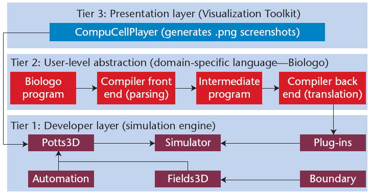
CompuCell3D’s architecture. We can modify, extend, or replace any tier without affecting the other tiers.

Tier 1: CompuCell3D’s Core

The CPM is the core of CompuCell3D’s framework, and it’s designed to accurately simulate cell interactions and movement. Specifically, it uses a lattice to describe cells and then associates an integer index with each lattice site (voxel) to identify each cell’s spatial extent and location at any given instant. The index value at a lattice site is σ if the site lies in cell σ. Domains in the lattice—that is, collections of lattice sites with the same index—represent cells, so a cell is thus a set of discrete components that can rearrange to produce cell-shape changes and motion.

Instead of representing the forces that cause cells to rearrange directly, the CPM aggregates them into an effective energy E, the gradient of which is the force acting at any point. Because of these forces and the cellular environment’s effectively infinite viscosity (no inertia), the cells gradually rearrange to reduce the pattern’s generalized energy. The effective energy contains terms describing cell interactions, motion under cytoskeletal fluctuations, and response to external chemical stimuli; its parameters change during cell growth, death, division, and differentiation. We use the term effective energy because it contains terms that mimic energies (for example, a cell’s response to a chemotactic gradient). Equation 1 shows a typical energy E:

$$E=E_{\mathrm{Contact}}+E_{\mathrm{Volume}}+E_{\mathrm{Surface}}+E_{\mathrm{Chemical}}·$$ (1)

A modified Metropolis algorithm for Monte Carlo Boltzmann dynamics implements cell membrane fluctuations (each term describes a different biological mechanism). The contact energy describes the net adhesion and repulsion between two cell membranes and is the product of the binding energy per unit area and the total area. Volume and surface energy terms implement constraints on cellular volume and surface area, respectively—they’re quadratically proportional to a cell’s current volume (surface area) and a target value, which can vary between cell types. Chemical energy can result from cellular chemotaxis, or oriented movement, toward an external chemical gradient, or haptotaxis, which restricts reactions to a selected set of cell types.

We used the Facade design pattern¹ to implement the CPM. A Facade pattern defines a common interface for unrelated objects, enabling them to interact without prior knowledge of their internals. Potts3D—our reference implementation of the generic CPM—uses the Facade pattern and consists of collections of objects or modules that work together to implement specific functionality. Using a standardized interface for our modules ensures that we can upgrade them without a complete redesign of Potts3D.

Cell structure and differentiation

In both mathematical and computational modeling, the biological cell provides a useful level of abstraction that hides subcellular details.³ We use a standard object model to represent cells, treating each cell as an object with certain attributes.

During morphogenesis, cells differentiate from initial multipotent stem cells into specialized cell types; this qualitative change in cell behavior is generally abrupt and irreversible. We use a variation of the State design pattern,¹ which lets an object alter its behavior when its internal state changes, to implement cell differentiation via the Automaton module. Instead of defining abstractness for states, we define abstract transitions—specifically, abstracting functionality for transitioning to a particular state. In the presence of irreversible type changes, this design saves PSE size because the number of required classes grows linearly with the number of states that have incoming transitions as opposed to the number of states in general. During the simulation, we evaluate a list of possible transitions whenever a cell changes position or site to determine if the cell’s state has changed. If so, we change the cell’s type; otherwise, its state remains unchanged.

Lattice representation

CompuCell3D simulations run on a lattice, as in Figure 2.⁴ Consider a relatively small 200³-pixel lattice, with each pixel consuming a very conservative 32 bits; in three dimensions, a naive implementation of the lattice requires approximately 128 Mbytes of memory. Because cells in CompuCell3D are collections of pixels, we associate with every pixel a pointer to a cell object (instead of storing an instance of a cell object in every pixel). Assuming an average cell to be a collection of 25 pixels, our lattice implementation uses approximately 30 percent of the memory required in the naive implementation. Memory savings increase with increasing average cell size.

Figure 2.

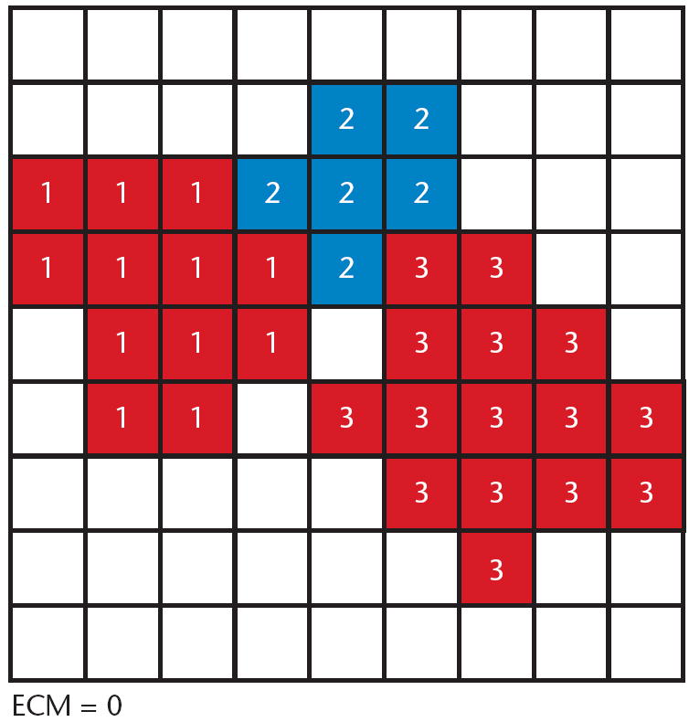
Example lattice in CompuCell3D. This lattice contains three cells, consuming lattice locations labeled 1, 2, and 3. Different cells (such as 1 and 3, shaded the same color for clarity) might have the same type. All other lattice locations are labeled 0 to designate the Extracellular Matrix (ECM).

In our implementation, we abstract the Field3D module such that the lattice implementation can use its own data structure to represent the lattice itself (as hexagonal or square, for example), which lets the Field3D module support different types of lattices without modifying the basic interface. In addition, Field3D can enforce user-defined boundary conditions (using the Boundary module) along each individual lattice axis. We use the Factory Method design pattern¹ to promote loose coupling between the CPM lattice and the boundary strategy because it models an interface for creating an object, which at the time of instantiation lets its subclasses decide which object to create. The user subsequently inputs each axis’s boundary strategy, which is instantiated accordingly at runtime.

Supporting multiple features

CompuCell3D also lets users add or remove functionality from a simulation. A biologist might want to observe cell behavior with and without cell division, for example, and an appropriate plug-in can implement that option. Plug-ins provide a clear structure for extending the simulation framework—fortunately, adding features through plug-ins doesn’t affect the framework’s core functionality. Table 1 lists the features available in CompuCell3D; it shows plug-ins that operate at the field level of modeling (such as PDE solvers), and those that operate at the cell level, controlling individual cells’ properties.

Table 1.

Selected CompuCell3D plug-ins.

Name	Function
AdvectionDiffusionSolver	Solves an advection-diffusion equation on a cell field.
FlexibleDiffusionSolver	A customizable solver of diffusion equations that also allows secretion, absorption, and diffusion restriction by cell type. Also allows variable space step, time step, diffusion constants, secretion rates, and number of fields.
BoundaryPenalty	Enforces an energy penalty if a cell is close to a boundary, to prevent cells spreading on domain boundaries.
CellBoundaryTracker	Provides locations of cell-boundary voxels.
CellVelocity	Tracks cell speeds.
CenterOfMass	Tracks cell centers of mass.
Chemotaxis	Implements cell chemotaxis to an external chemical field, with forces proportional to chemical gradients.
ExternalPotential	Imposes a directed potential, or force, on cells.
Growth	Implements a cell density-dependent algorithm for domain growth. The lattice maintains its current dimensions until cell density reaches a user-specified threshold, then it grows in positive z by a user-specified amount.
LengthConstraint	Implements anisotropic cells.
Mitosis	Implements cell division.
SimpleClock	Implements an internal timer for cells. Provides the ability to start a timer and decrement until it hits zero.
Viscosity	Implements cell viscosity (useful in fluid flow simulations).

Tier 2: Biologo

Biologo extends XML to model multiple morphogenesis subprocesses, including cell differentiation, volume constraints, intercellular adhesion, chemotaxis, haptotaxis, and reaction-diffusion. It inherits XML syntax and semantics using extended XML parsing libraries from Xerces (http://xml.apache.org/xerces-c/), which also gives it XML’s inherent extensibility. Biologo’s extensions for CompuCell3D are implemented as XML modules that convert transparently into dynamically loaded C++ plug-ins.

Translation of a Biologo program into the source code for a CompuCell3D plug-in is a two-stage process. The compiler front end parses and lexically analyzes the Biologo program, executes several error-checking routines, and generates an intermediate file containing simpler syntax, which then passes through the code generator that processes and translates the intermediate file into C++. The intermediate syntax opens the door for future implementation of a compiler that can implement machine-independent optimizations during generation of the intermediate representation, which is uniform across architectures (unlike C++ code, which can be nonuniform). Intermediate code saves the overhead of having to change the code generator front-end modules to suit each platform on which we deploy CompuCell3D.

Tier 3: The CompuCellPlayer

One major task of PSEs is to supply intuitive GUIs and visualization tools, but scientific developers often neglect this area of software development or treat it as a back-burner task. Early versions of CompuCell3D lacked a GUI and outsourced visualization to third-party external tools, but by definition a PSE requires an easy and understandable interface for user interaction.

To address these issues, we developed a tool called CompuCellPlayer to provide visualization services and a front end to CompuCell3D. It displays the current simulation state in real time on the user’s screen and saves the state in the form of a graphical .png file on the hard drive for further postprocessing. CompuCellPlayer also lets users render objects in 2D and 3D, display chemical concentrations, pressures, and cell velocity fields, zoom in or out, and toggle cell border display.

CompuCellPlayer is fully customizable and lets users configure cell colors and borders as well as concentration and vector-field plots. Based on the XML simulation description, the CompuCellPlayer chooses and enables plots appropriate for the simulation. Another useful feature is its ability to save multiple simulation views during a single run—including the cell, chemical, and velocity fields, in the form of screenshots—without having to repeat the simulation. Overhead for this operation is negligible.

The CompuCellPlayer can also run in noninteractive or silent mode, which is important when users run CompuCell3D on clusters accessed through queuing systems that don’t run interactive jobs. In this case, users must prepare a screenshot description text file to tell the CompuCellPlayer which views to save so it can prepare the screenshot description file. The user simply switches views and presses the Camera button on the views that should be saved. At the end of this step, CompuCellPlayer stores a screenshot description file that can control the CompuCellPlayer in noninteractive mode.

Finally, users can serialize the entire simulation to restart at a later time, possibly with different parameters. This particular feature makes it possible to equilibrate cellular patterns before running a simulation, from a more physically relevant initial state.

Applications

A flexible morphogenesis PSE should be able to represent multiple types of simulations, organisms, chemical fields, reaction-diffusion PDEs, cell types, and so on. We can demonstrate CompuCell3D’s flexibility by illustrating three biologically relevant test simulations. We provide XML for each example at www.nd.edu/~lcls/compucell/examples.htm.

Cell-Sorting Simulation

Embryonic cells of two different types, when dissociated, randomly mixed, and reaggregated, can spontaneously sort to reestablish coherent homogeneous tissues. Both complete and partial cell sorting (in which large clusters of one cell type are engulfed or surrounded by a continuous layer of cells of the other cell type) occur during in vitro experiments via embryonic cells. Cell sorting is a key step in regenerating a normal animal from aggregates of dissociated cells of adult hydra⁵ and in establishing spatial relationships among cells during embryogenesis in all species. Biologically, cell sorting is thought to result from adhesivity differences.⁶ CompuCell3D lets researchers study how differential cell adhesion drives cells to produce different patterns. Even cell sorting between two different initially randomly distributed cell types (as in Figure 3a), for example, results from having one cell type stick strongly to itself (as in Figure 3b). If cells stick most strongly to cells of the opposite type, a checkerboard pattern forms (see Figure 3c).

Figure 3.

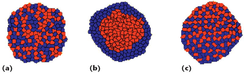
Cell sorting. Starting from (a) a randomly mixed two-cell-type aggregate, we arrive at different final state patterns for different cell–cell adhesivity settings. (b) Cells adhere to other cells of the same type, with the more adhesive cell type (red) clustering at the center. (c) A checkerboard pattern forms due to preferential adhesion between cells of different types.

The XML code in Figure 4 shows a CompuCell3D configuration file for cell sorting. Changing the adhesivity values in the Contact plug-in produces different patterns.

Figure 4.

CompuCell3D configuration file for cell sorting. Different adhesivity settings are shown in the Contact plug-in; other plug-ins for center of mass, volume, and surface area calculations are also displayed along with Cellular Potts Model (CPM) parameters at the top.

Chondrogenic Condensation Simulation

Following other research,^4,7 we can model the spatiotemporal patterning of cells during cartilage formation (called chondrogenesis) in a growing embryonic chicken limb. We use an initially uniform distribution of cubic cells and superimpose a chemoattractant, which we identify with transforming growth factor-beta (TGF-β), a molecule that acts as an activator in pattern formation.

We implement cell differentiation as a cell type map (CTM), an automaton consisting of a set of cell types and rules for type transitions. As an example, we can illustrate the CTM other researchers⁴ used in their avian limb-bud growth model in Biologo, employing two different types of cells: noncondensing and condensing, with the latter much more adhesive than the former. A high concentration of an activator chemical (above a threshold) stimulates a type change from noncondensing to condensing, and a low concentration stimulates the reverse transition, as in Figure 5. All CTMs define a medium cell type to represent the ECM; Figure 6a (p. 56) defines this CTM using Biologo. The useplugin tag includes the LimbChemical effective energy, enabling access to its inputs and fields using the “.” operator. In this case, we reference the LimbChemical.activator field and the LimbChemical.Threshold. The CTM specifies each cell type and includes an updatecelltypes module to specify the conditions for cell differentiation to this type. Figure 6b instantiates this CTM in the CompuCell3D configuration file.

Figure 5.

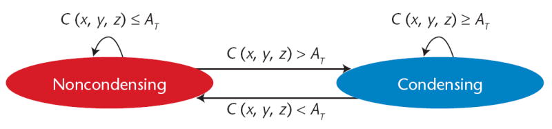
Cell type map for an avian limb simulation. A noncondensing cell becomes condensing when exposed to an activator concentration C(x, y, z) above a threshold, and a condensing cell becomes noncondensing when exposed to an activator concentration below a threshold.

Figure 6.

Adding a cell type map (CTM) to CompuCell3D with Biologo. (a) CTM for a chondrogenic condensation simulation with two cell types, condensing and noncondensing. (b) Instantiation of the avian limb CTM in the CompuCell3D configuration file.

Building on this approach, we can also use Biologo to add a CPM effective energy term or Hamiltonian to simulate haptotaxis, which depends on two superimposed chemical fields in other research.⁴ The first represents TGF-β, which induces an inhibitor that acts laterally to the condensations, thus generating the stripe-like patterns observed in avian limb chondrogenesis. We populate the TGF-β with a reaction-diffusion equation solver.⁸ TGF-β then stimulates cells to secrete an adhesive glycoprotein—called fibronectin (the second field)—which locally traps cells in clusters by haptotaxis in a process known as mesenchymal condensation. The haptotaxis effective energy plug-in implements Equation 2 for the fibronectin concentration C:

$$E_{\mathrm{Chemical}}=\sum _{\mathbf{x}}{\mu }_{\sigma \left(\mathbf{x}\right)}C\left(\mathbf{x},t\right).$$ (2)

Biologically, only the active zone cells exposed to a high activator concentration can produce fibronectin. We add this functionality through the Biologo Hamiltonian in Figure 7a (p. 57). The user specifies the value of an activator threshold that, if exceeded, stimulates fibronectin secretion, the scaling factor μ from Equation 2, and the rate of secretion. The ConcentrationFile is a binary file of floating-point values populating the activator chemical field, with x as the innermost loop. Figure 7b is a CompuCell3D configuration file snippet that adds the customized haptotaxis extension to a simulation, thereby specifying all input values. The Hamiltonian step module specifies the rates of chemical secretion and resorption, modifying its associated field. In this case, we secrete a quantity FibroRate into fibronectin if the corresponding activator concentration is above or equal to Threshold. The effective energy equation sums over all lattice locations pt (predefined), but only condensing cells contribute.

Figure 7.

Adding an effective energy term to CompuCell3D with Biologo. (a) LimbChemical effective energy or Hamiltonian for the avian limb-bud growth simulation. The effective energy is associated with two chemical fields: activator (populated through a ConcentrationFile) and fibronectin (populated by cell secretion and resorption) superimposed on the Cellular Potts Model (CPM) lattice. (b) Sample instantiation of the Biologo-generated LimbChemical plug-in for a CompuCell3D configuration file.

The effective energy includes cell–cell adhesion, volume and surface area constraints, and haptotaxis from Biologo. CompuCell3D can also simulate chicken limb formation on an irregular domain or on a growing regular domain. Figure 8 shows the results of this latter simulation.

Figure 8.

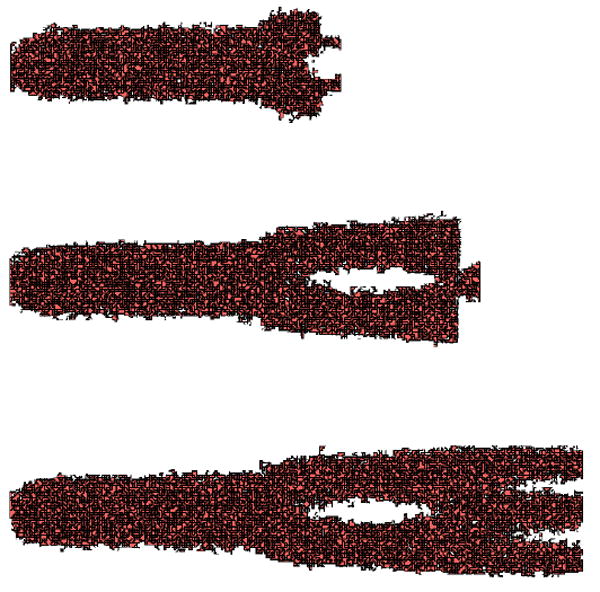
Avian limb development, visualizing only condensing cells for clarity. The limb forms at the center of a 3D box of cells and is surrounded by mostly noncondensing cells. Formation begins with the humerus after 2,300 Monte Carlo steps (MCSs), followed by the radius and ulna after 3,250 MCSs, and finally digits after 4,250 MCSs.

Simulating in vitro Capillary Development

Merks and his colleagues⁹ developed an in silico model of the widely used human umbilical vascular endothelial cells (HUVEC) in vitro for blood vessel growth (called angiogenesis). During the first steps of embryonic vascular development, endothelial cells (ECs, the cells that line the inner walls of blood vessels) organize into polygonal patterns of cell cords. Existing vessels subsequently sprout and split, forming new blood vessels and remodeling the initial vascular network. Merks and his colleagues assumed that ECs secrete a morphogen that the ECM inactivates, extend filopodia up the morphogen gradients, and elongate in response to angiogenic growth factors.

Biologo uses PDEs to model the reaction and diffusion of secreted, diffusible, and nondiffusible molecules.⁸ Such cellular models typically represent cells’ production of and responses to diffusing molecules as sets of PDEs. Nian Li and his colleagues¹⁰ demonstrated convergence and stability of the finite difference method for solving reaction-diffusion equations. A user can write a set of PDEs in Biologo to generate a 2D finite difference solver plug-in that a CompuCell3D configuration file can subsequently dynamically load, to populate an associated chemical field for use by other CompuCell3D plug-ins. For our experiments, we modeled in vitro capillary development, duplicating the results of another model⁹ and, by analogy to the Gamba-Serini PDE model,¹¹ simulating the chemoattractant c’s reaction-diffusion in Equation 3:

$$\frac{\partial c}{\partial t}=\alpha {\delta }_{{\sigma }_x,0}-\left(1-{\delta }_{{\sigma }_x,0}\right)\epsilon c+D{\nabla }^{2}c,$$ (3)

where α is the rate at which cells secrete the chemoattractant, ε is the rate of chemoattractant resorption in ECM, D is the diffusion constant of the chemoattractant in both cells and ECM, and δ_σx,0 is 1 for cells and 0 for the medium. Hence, c diffuses and decays in the extracellular matrix.

This equation models a chemoattractant’s diffusion and breakdown and thus doesn’t autonomously drive cell patterning. Patterns form due to the close interplay between cell migration and chemoattractant secretion and decay. Figure 9a (p. 58) shows this vasculogenesis model in Biologo. DiffEq tags represent each PDE, and each tag evolves one field with time. An equation specifies each unique term separately. Kronecker is equivalent to δ(σ(x, y, z), 0), which is 1 if point (x, y, z) corresponds to a medium point and 0 if (x, y, z) lies in a biological cell; Laplacian computes the Laplacian of the passed field. Each solver predefines user inputs for the time step and number of steps in the finite difference algorithm. These parameters, along with α, ε, and D, are instantiated in the CompuCell3D configuration file as shown in Figure 9b, which also shows the instantiation of a chemotaxis plug-in using the field c from the Gamba-Serini PDE solver. Numbers of PDE steps per CPM step, the time step, and the space step for the finite difference method are also specified.

Figure 9.

Adding a partial differential equation (PDE) solver to CompuCell3D with Biologo. (a) A hybrid model of angiogenesis,⁹ derived from the Gamba-Serini PDEs,¹¹ implemented in Biologo as an evolver of chemical fields. (b) Instantiation of this solver in the CompuCell3D configuration file. The CompuCell3D chemotaxis plug-in also accepts ChemotaxisByType tags with attributes for cell type and associated Lambda values.

For more complete 3D PDE solving ability, an alternative is to embed Python code and use FiPy (www.ctcms.nist.gov/fipy/) calls within Biologo between Python tags. We use source and transient diffusion terms from the FiPy libraries to set up the equivalent version of Gamba-Serini PDEs in Figure 10. This also provides the ability to discretize multiple fields differently in time by passing different dt values to solve(). Once again, we reference Kronecker. Embedded FiPy offers a trade-off in representative power for performance, yielding roughly a six-fold performance slowdown versus Biologo’s generated C++.

Figure 10.

Python. This Biologo representation of the PDE model in Figure 9a uses embedded FiPy.

Figure 11 (p. 59) shows a CompuCell3D version of the in vitro capillary development model. A surface tension γ = J_Cell,Medium − J_Cell,Cell/2 determines whether cells cohere (γ > 0) or dissociate (γ < 0). Figure 11a includes a cell-length constraint that causes cells to elongate, which is represented with an extra term in the CPM Hamiltonian that’s quadratically proportional to the deviation between a cell’s current and target length L. In this figure, L = 30, which results in a connected network with thinner chords. We also implemented a constraint⁹ to preserve local cell connectivity and removed cell adhesion by setting J_Cell,Cell = 60 and J_Cell,Medium = 30, yielding γ = 0. As long as elongation is present, the HUVEC forms networks even in the absence of adhesion. Figure 11b shows the chemical field from Equation 3 added through Figure 9a, now recognized and visualized through the CompuCellPlayer, along with superimposed cell boundaries. Finally, Figure 11c enforces rounded cells (L = 10) and shows that a network doesn’t form due to the lack of cell stretching, in accordance with other results.⁹

Figure 11.

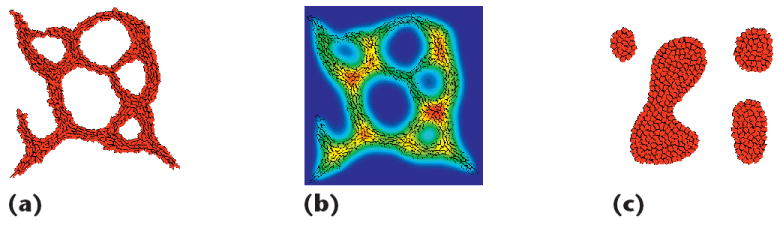
Output of in vitro capillary development simulations. (a) Elongated cells (L = 30) in the absence of cell adhesion, showing the capillary networks found in other research.⁹ (b) Chemical concentration from the same simulation, visualizing the field added through Biologo. (c) Vascular islands forming due to the enforcement of rounded cells (L = 10).

Performance

Let’s now examine how CompuCell3D performance scales with cell density and lattice size (in voxels) for a cell-sorting simulation run for 500 Monte Carlo steps (MCSs). Figure 12a uses a constant 50 × 50 × 50 lattice size, whereas Figure 12b uses a constant cell density of 27 percent. We conducted our tests on an HP workstation with an Intel Pentium IV 3.2-GHz processor and 1 Gbyte of memory that ran Red Hat Linux 9.0, kernel 2.4.21. The C++ compiler was g++ version 3.2.3. As we would expect, execution time scales linearly with lattice size at constant density. In the future, we hope to improve scaling with cell density in two ways: by recognizing sparse areas of the lattice with the help of sophisticated data structures (to keep track of cellular positions and avoid neutral or ineffective flip attempts) or by implementing the random-walk algorithm,¹² which restricts flip attempts to boundary lattice locations.

Figure 12.

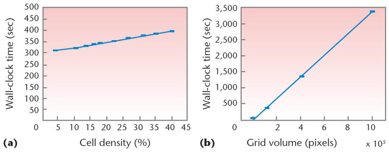
Comparisons of wall-clock execution time versus cell density (constant lattice size of 50 × 50 × 50 voxels) and lattice size (constant cell density of 27 percent). We ran five simulations for each test, and show the mean execution time along with error bars for mean deviation.

In our next release and upgrade of CompuCell3D, we will add a layer to the PSE that will implement Python scripting as another option for user interaction. This layer will balance interactive power with the abstraction level—the interface will be more complex than Biologo, but a larger set of behaviors will be modifiable. We’ll also wrap C++ libraries from CompuCell3D with SWIG, a useful tool for converting C++ functionality into importable Python modules, and group importable modules into packages that the user can subsequently import as high-level functions to invoke backend functionality. A prototype version is currently available at www.nd.edu/~lcls/compucell/downloads.htm. Finally, we plan to incorporate a parallel CPM implementation into the PSE using domain decomposition to accommodate larger simulations and to make a Windows-compatible binary available.

Although we focused on biological applications in this text, the benefits of PSEs have been proven to extend to other domains as well, such as multiway data modeling¹³ and workflow setup for grid environments.¹⁴ Another classic example is Interactive ELLPACK,¹⁵ which extended the ELLPACK language to provide a graphical interactive environment for PDE solving. Despite their wide range of applications, these PSEs succeed in a similar fashion by removing the burden of low-level modular architectural concerns off the users, freeing them up to operate at a level of abstraction suitable for their expertise.

Biographies

Trevor Cickovski is a graduate student and research assistant in the Department of Computer Science and Engineering at the University of Notre Dame. His research lies in morphogenesis modeling, molecular modeling, and domain-specific language design. Cickovski has an MS in computer science and engineering from the University of Notre Dame. He is a member of the ACM and the IEEE. Contact him at tcickovs@nd.edu.

Kedar Aras is an engineer in the corporate innovation technology division at Whirlpool. His research interests are in computational biology and bioinformatics, software engineering, and systems neuroscience and neuroengineering. Kedar has an MS in computer science from the University of Notre Dame. Contact him at kedar. aras@gmail.com.

Maciej Swat is a research associate in the Biocomplexity Institute at Indiana University. His research lies in computational biophysics and scientific problem-solving environments. Swat has a PhD in physics from Indiana University. He is a member of the Biophysical Society. Contact him at mswat@indiana.edu.

Roeland M.H. Merks heads the plant systems modeling group in the plant systems biology department at the Flanders Institute of Biotechnology and Ghent University, Belgium. His research interest is in biological morphogenesis modeling, including cell-based modeling of plant development, coral growth, and vascular development in mammals. Merks has a PhD in computational science from the University of Amsterdam. He is a member of the American Physical Society and of the European Society for Mathematical and Theoretical Biology. Contact him via www.roelandmerks.nl.

Tilmann Glimm is an assistant professor of mathematics at Western Washington University. His research interests include analytical and numerical methods in nonlinear partial differential equations with applications in developmental biology. Glimm has a PhD in mathematics from Emory. He is a member of SIAM and the American Mathematical Society. Contact him at glimmt@wwu.edu.

H. George E. Hentschel is a professor of physics at Emory University. His research interests include nonequilibrium statistical mechanics, computational biophysics, information processing, and dynamical systems. Hentschel has a PhD in theoretical chemistry from Cambridge. He is a fellow of the Cambridge Philosophical Society and a member of the American Physical Society and the American Association for the Advancement of Science. Contact him at phshgeh@physics.emory.edu.

Mark S. Alber is the Endowed Chair in Applied Mathematics and a professor of physics at the University of Notre Dame, where he also serves as director of the Center for the Study of Biocomplexity. His research interests are in mathematical and computational biology. Alber has a PhD in mathematics from the University of Pennsylvania. Contact him at malber@nd.edu.

James A. Glazier is a professor of physics, adjunct professor of informatics and biology, and director of the Biocomplexity Institute at Indiana University; president of SpheroSense Technologies; and vice chair of the American Physical Society’s Division of Biological Physics. His research interests include both experimental and computational developmental biology, computational modeling, biomedical problems, and liquid foams. Glazier has a PhD in physics from the University of Chicago. He is a fellow of the Institute of Physics (London) and the American Physical Society. Contact him at glazier@indiana.edu.

Stuart A. Newman is a professor of cell biology and anatomy at New York Medical College. His research interests include the development of the vertebrate limb and the origination and evolution of animal form. Newman has a PhD in chemical physics from the University of Chicago. He coauthored Biological Physics of the Developing Embryo (Cambridge, 2005). Contact him at stuart_newman@nymc.edu.

Jesus A. Izaguirre is an associate professor of computer science and engineering at the University of Notre Dame. His research interests include molecular dynamics, Monte Carlo methods, cellular automata, and the analysis of biological networks. Izaguirre has a PhD in computer science from the University of Illinois at Urbana-Champaign. He is a member of the IEEE and the IEEE Computer Society. Contact him at izaguirr@cse.nd.edu.

References

- 1.Gamma E, et al. Design Patterns: Elements of Reusable Object-Oriented Software. Addison-Wesley; 1995. [Google Scholar]
- 2.Merks RMH, et al. Problem-Solving Environments for Biological Morphogenesis. Computing in Science & Eng. 2006;8(1):61–72. [Google Scholar]
- 3.Merks RMH, Glazier JA. A Cell-Centered Approach to Developmental Biology. Physica A. 2005;352(1):113–130. [Google Scholar]
- 4.Cickovski T, et al. A Framework for Three-Dimensional Simulation of Morphogenesis. IEEE/ACM Trans Computational Biology and Bioinformatics. 2005;2(4):273–288. doi: 10.1109/TCBB.2005.46. [DOI] [PubMed] [Google Scholar]
- 5.Graner F, Glazier JA. Simulation of Biological Cell Sorting Using a Two-Dimensional Extended Potts Model. Physical Rev Letters. 1992;69(13):2013–2016. doi: 10.1103/PhysRevLett.69.2013. [DOI] [PubMed] [Google Scholar]
- 6.Glazier JA, Graner F. Simulation of the Differential Adhesion Driven Rearrangement of Biological Cells. Physical Rev E. 1993;47(3):2128–2154. doi: 10.1103/physreve.47.2128. [DOI] [PubMed] [Google Scholar]
- 7.Chaturvedi R, et al. On Multiscale Approaches to 3-Dimensional Modeling of Morphogenesis. J Royal Soc Interface. 2005;2(3):237–253. doi: 10.1098/rsif.2005.0033. [DOI] [PMC free article] [PubMed] [Google Scholar]
- 8.Hentschel HGE, et al. Dynamical Mechanisms for Skeletal Pattern Formation in the Vertebrate Limb. Proc Royal Soc London B. 2004;271(1549):1713–1722. doi: 10.1098/rspb.2004.2772. [DOI] [PMC free article] [PubMed] [Google Scholar]
- 9.Merks RMH, et al. Cell Elongation Is Key to in silico Replication of in vitro Vasculogenesis and Subsequent Remodeling. Developmental Biology. 2006;289(1):44–54. doi: 10.1016/j.ydbio.2005.10.003. [DOI] [PMC free article] [PubMed] [Google Scholar]
- 10.Li N, Steiner J, Tang S. Convergence and Stability Analysis of an Explicit Finite Difference Method for 2-Dimensional Reaction-Diffusion Equations. J Australian Mathematical Soc B. 1994;36(2):234–241. [Google Scholar]
- 11.Gamba A, et al. Percolation Morphogenesis and Burgers Dynamics in Blood Vessel Formation. Physical Rev Letters. 2003;90(11):118101. doi: 10.1103/PhysRevLett.90.118101. [DOI] [PubMed] [Google Scholar]
- 12.Gusatto E, et al. An Efficient Parallel Algorithm to Evolve Simulations of the Cellular Potts Model. Parallel Processing Letters. 2005;15(1):199–208. [Google Scholar]
- 13.van Stokkum IHM, Bal HE. A Problem Solving Environment for Interactive Modeling of Multiway Data. Concurrency and Computation: Practice and Experience. 2005;18(2):263–269. [Google Scholar]
- 14.Currle-Linde N, et al. Proc Int’l Conf ParCo 2005. Central Inst for Applied Mathematics; 2005. Science Experimental Grid Laboratory (SEGL) Dynamical Parameter Study in Distributed Systems; pp. 49–56. [Google Scholar]
- 15.Dyksen WR, Ribbens CJ. Interactive ELLPACK, An Interactive Problem Solving Environment for Elliptic Partial Differential Equations. ACM Trans Mathematical Software. 1987;13(2):113–132. [Google Scholar]