Model criticism based on likelihood-free inference, with an application to protein network evolution

Abstract

Mathematical models are an important tool to explain and comprehend complex phenomena, and unparalleled computational advances enable us to easily explore them without any or little understanding of their global properties. In fact, the likelihood of the data under complex stochastic models is often analytically or numerically intractable in many areas of sciences. This makes it even more important to simultaneously investigate the adequacy of these models—in absolute terms, against the data, rather than relative to the performance of other models—but no such procedure has been formally discussed when the likelihood is intractable. We provide a statistical interpretation to current developments in likelihood-free Bayesian inference that explicitly accounts for discrepancies between the model and the data, termed Approximate Bayesian Computation under model uncertainty (ABCμ). We augment the likelihood of the data with unknown error terms that correspond to freely chosen checking functions, and provide Monte Carlo strategies for sampling from the associated joint posterior distribution without the need of evaluating the likelihood. We discuss the benefit of incorporating model diagnostics within an ABC framework, and demonstrate how this method diagnoses model mismatch and guides model refinement by contrasting three qualitative models of protein network evolution to the protein interaction datasets of Helicobacter pylori and Treponema pallidum. Our results make a number of model deficiencies explicit, and suggest that the T. pallidum network topology is inconsistent with evolution dominated by link turnover or lateral gene transfer alone.

In the quest to comprehend complex observations, hypotheses about underlying mechanisms are formalized in terms of precise mathematical models (1). Much of statistical reasoning then proceeds in an iterative process between data acquisition, data analysis, and model development (2). At the i th iteration, the interpretation of observed data x₀ in terms of some target parameters θ conditional on a tentative, probabilistic model M_i has a long tradition in Bayesian inference (3). The focus is typically on the posterior density f(θ | x₀,M_i), which is related to the likelihood f(x₀ | θ,M_i) and the prior π_θ(θ | M_i) via Bayes' Theorem:

To explore whether the current model M_i is consonant with x₀, and to guide further model development, Bayesian predictive diagnostics (4, 5) ask whether x₀ can be viewed as a random observation from a predictive distribution m(x|M_i) in terms of a chosen discrepancy function ρ(x,x₀), x ∼ m; interpretation of such diagnostics has been the subject of lively debate (6, 7). Application of this machinery for complex models is provided by the workhorses of Bayesian inference (8), such as Markov Chain Monte Carlo (MCMC), as long as the likelihood is readily evaluable up to a normalizing constant.

In many areas of science, such as econometrics (9), molecular genetics (10), epidemiology (11), and evolutionary systems biology (12), the likelihood is sometimes intractable. Nevertheless, given a value of θ, it is typically easy to simulate data from f(·|θ,M_i). Approximate Bayesian Computation (ABC), reviewed in ref. 10, proposes to infer θ by comparing simulated data x to the observed data x₀, in terms of a (real-valued) univariate discrepancy ρ that combines a set of (computationally tractable) summaries s= (S₁,…,S_k,…,S_K). In its simplest form, values of θ for which the discrepancies are within τ ≥ 0 are retained to define the “approximate likelihood”

in the sense that as τ → 0, t_τ(θ) should approach the likelihood of the summaries, f(s(x₀)|θ,M_i); see Fig.1A and the supporting information (SI) Appendix, subsection S1.2. ABC may be embedded into Bayesian methods to formally select one model from a specified collection of models, or to average them (13–15); see Fig. 1B. However, relative comparisons between models do not convey whether models correspond adequately to the observed data and, without exploring the adequacy of models to explain the data, the meaning of reporting θ from Eq. 2 remains unclear, see Fig. 2.

Fig. 1.

Comparison of ABC versus our implementation of likelihood-free inference, on a fictitious PIN dataset x₀, fictitious models with a single, common parameter θ, and one summary, DIAM, with observed value 13. The points represent posterior samples of θ and DIAM and resemble more a “bouncy castle” than a likelihood surface. (A) In “standard” ABC, inference proceeds by retaining those samples (blue triangles) for which the realized errors are smaller than τ (here, τ = 2), and are taken to approximate the posterior density of θ (Top). (B) In “standard” ABC, different models (blue, red, yellow) may be compared based on the number of retained samples under one model relative to that number under all other models (Top Left), for instance, in terms of the log odds ratio (Top Right), here indicating that model M₃ performs best. (C) We propose to use the generated data to a fuller extent by augmenting the likelihood (vertical dimension, ɛ). Discrepancies between the data and the models are made explicit in terms of posterior quantities of ɛ.

Fig. 2.

N(θ, 1) toy example to illustrate our approach to diagnose model mismatch with posterior densities of multiple error terms when the likelihood is intractable. Suppose we have obtained a dataset x₀ of 200 independent samples. We believe each sample of x₀ to be generated from f(·|θ,M₁) = N(θ, 1) with θ unknown, whereas in reality x₀ is exponential with rate θ_t = 0.2 (denoted with M_t). By construction, the sample mean (MEAN) is a sufficient statistic to estimate both θ and θ_t. To illustrate one iteration of ABCμ, suppose we sample θ = 3, ɛ_MEAN = −0.94 from the priors (respectively, uniform and exponential). We generate 50 errors $\overline{x_b}-\overline{x_0}$ (A, red points for x_b ∼ f(·|θ = 3,M₁)), estimate the associated error density ξ̂(·;x) (A, black line) with a biweight kernel, and compute ξ̂(ɛ_MEAN;x) (A, blue point). Using algorithm ABCμ, we estimated posterior quantities of θ and ɛ under various summary statistics. Summarizing x only with MEAN, the method indicates no model mismatch (B, row 1, column 2; 95% high posterior density interval (HPD)) and θ is estimated as if x₀ were indeed N(1/θ_t, 1) (B, row 1, columen 1; posterior mean). Reminding ourselves that likelihood-free inference is honest in that inference is here based on $\overline{x_b}-\overline{x_0}$, we see that the algorithm samples correctly from Eq. 9. Observing that under M₁ the standard deviation (SD) is 1 independently of θ and that SD is 1/θ_t under M_t, we recognize that progress is possible when a comprehensive set of summaries is employed. Repeating our method based on MEAN, SD, and the 0.25 quantile (QU0.25), targetting Eq. 9, we find that all error terms indicate model mismatch (B, row 2, column 2-4; and C, posterior error densities for 4 runs of ABCμ starting from overdispersed initial values (colored solid lines) versus the (dashed) prior π_ɛκ(ɛ_κ|M_i)). If posterior quantities of comprehensive error terms clearly diagnose model mismatch as in this example, we recommend questioning the interpretability of θ|x₀ in terms of the likelihood model. For reference, we applied standard (Rejection) ABC to this example; conditioning on the summaries MEAN, SD, and QU0.25, we find that the numerical estimates of θ|x₀ agree between ABC and ABCμ (with τ fixed as in B, third row).

We continue in believing that “all models are wrong but some are useful” (2), which prompts us to interpret several ρ_k(S_k(x),S_k(x₀)) as realizations of real-valued error terms, denoted by ɛ = (ɛ₁,…,ɛ_K) (16). Error terms are not observed, and must be estimated from the data; we develop a theoretical framework and provide an algorithm, ABCμ, for this purpose when the likelihood is intractable. We intentionally focus on the posterior distributions of components of ɛ to make probabilistic statements of mismatch between the model and the data (17) and hence to facilitate model criticism, as summarized in Fig. 1C.

Postgenomic data such as protein interaction networks (PINs) are now available for a growing number of organisms, (e.g., refs. 18 and 19). They offer a new perspective on the function of all organisms, and are, in addition to individual gene or genomic approaches, increasingly useful to elucidate the evolution of living systems, (e.g., refs. 12, 20, and 21), despite being noisy, incomplete, and static descriptions of the real, transient protein network (22). To elucidate the network evolution of prokaryotes, we here analyze the compatibility of the Treponema pallidum and Helicobacter pylori PIN datasets with a set of competing models inspired by fundamentally different modes of network evolution.

ABC under Model Uncertainty*

Joint Posterior Density of Model Parameters and Summary Errors.

For the purpose of model criticism in situations where the likelihood is intractable, define the unknown error ɛ as the random variable with conditional probability distribution

Next, we assume that ℙ_θ,x0(ɛ ≤ e) has a density ξ_{θ, x0} with respect to an appropriate measure for ρ.† It is natural to suggest using this quantity as an augmented likelihood for x₀ under ρ while adhering to the current model,

We thus capture the direct information brought by the discrepancies ρ on θ and/or model M_i in a scalar value. For a given prior π_θ,ɛ(θ,ɛ|M_i), we embrace two aspects of statistical reasoning, parameter inference and model criticism, simultaneously by the joint posterior density

using the data once.‡ In practice, we take π_θ,ɛ = π_ɛ × π_θ,§ reflecting our inability to quantify a priori model adequacy for a value of θ. The posterior relationship Eq. 5 exploits the dependence between model error and model parameterization. ABC only infers model parameterization from realized model errors after simulation and does not question the adequacy of the likelihood model.

The simplest algorithm to sample from Eq. 5 is:

Std-ABCμ1 Sample θ ∼ π_θ(θ | M_i), simulate x ∼ f(· | θ,M_i) and compute ɛ = ρ(s(x),s(x₀)).

Std-ABCμ2 Accept (θ,ɛ) with probability proportional to π_ɛ(ɛ | M_i), and go to Std-ABCμ 1.

Interpretation of the Marginals: Parameter Inference and Model Criticism.

The thrust of this article is to recognize the utility of the unknown error ɛ for model criticism. By design, nonzero values of ρ indicate discrepancies between the model and the data, so that intuitively, only if the model matches the data, we expect the mode of ξ_{θ, x0}(ɛ) to be on average zero for some value of θ if the summaries behave sufficiently well. Parameter inference based on the marginal posterior distribution f_ρ(θ|x₀,M_i) is justified in an “approximate likelihood” sense, because, under regularity assumptions (SI Appendix, S1.1) on ξ_{θ, x0}(ɛ) which we assume throughout this section,

Setting π_ɛ(ɛ|M_i) = 1{|ɛ| ≤ τ /2}/τ, we recover the “standard” ABC approximation Eq. 2; please see SI Appendix, S1.2 for more details and examples. We can interpret the variety of ABC kernels as exerting a particular prior belief on the adequacy of the current model (23). In agreement with methods of ABC (SI Appendix, S1.2), we always choose a prior π_ɛ(ɛ|M_i) with mode at zero to accommodate a prior belief that the model is plausible. For the purpose of parameter inference, it is sufficient to “plug-in” realized errors in Eq. 6, but here we also focus on the marginal posterior error f_ρ(ɛ|x₀,M_i). For the prior predictive error density L_ρ(ɛ) = ∫δ{ρ(s(x),s(x₀)) = ɛ}π(x|M_i)dx we have that

(see SI Appendix S1.1). Hence, f_ρ(ɛ|x₀,M_i) can be understood as an error density under the prior predictive distribution that is weighted according to error magnitude. Small error boosts the prior belief for a particular value of θ, see Eq. 6. We thus prefer model criticism based on Eq. 7 rather than L_ρ(ɛ) as it focuses on those θ actually inferred from the perspective of Eq. 5, and attenuates the dependence of L_ρ(ɛ) on π_θ(θ|M_i). This dependence is undesirable in that a faultless model could appear questionable under unfortunate prior choice (SI Appendix, S1.3). For the practitioner, we provide a computationally feasible method for model criticism within the prior predictive setting as an alternative to using data-splitting techniques that are here difficult or too expensive to construct (5, 7, 17).

Multidimensional Error Terms ɛ.

The complexity of the settings to which ABC is typically applied makes it difficult to think of a universal discrepancy function ρ. The joint posterior distribution of multiple errors ɛ = (ɛ₁,…,ɛ_K), corresponding to K discrepancies ρ_k(S_k(x),S_k(x₀)) (SI Appendix, S1.4), facilitates to diagnose model mismatch more systematically and comprehensively; we have

In the ABC literature, it has been recognized that attempting to match jointly a set of summaries is too conservative, and instead a linear combination of summaries is typically employed (14). Nonetheless, we believe that each summary captures aspects of model discrepancy. To control several summaries stringently for accurate and robust parameter inference (12), min_kξ_{k,θ, x0}(ɛ_k) here supersedes ξ_{θ, x0}(ɛ) (see Materials and Methods, section 3, and SI Appendix, S1.6).

Algorithm.

The major impediment in ABC—that the likelihood surface is turned into a “bouncy castle,” see Fig. 1—is in the multivariate case exacerbated by the fact that the unknown error terms are correlated by design, and easily outnumber the θ's. To obtain a smoothed, stabilized approximation to ξ_{k,θ, x0}(ξ_k) that better controls the volatility of the simulated datasets, we employ kernel density estimates ξ̂_k(ɛ_k;x):= 1/(Bh_k)∑_{b = 1}^BK([ɛ_k − ρ_k(S_k(x_b),S_k(x₀))]/h_k) in line with ABC (SI Appendix, S1.5). In theory, this corresponds to replacing ξ_{θ, x0}(ɛ) in Eq. 8 with min_k ∫h_k⁻¹K ((ɛ_k − ν_k)/h_k)ξ_θ,x0(v)dv. In practice (SI Appendix, S1.7), we set B = 50 and attain under technical modifications (see Material and Methods, section 3) a smoothing approximaion

on the auxiliary space (θ,ɛ,x). Various Monte Carlo strategies (8, 24) may be devised to sample from Eq. 9 (SI Appendix, S1.8); our MCMC implementation (SI Appendix, S1.9), particularly addresses the codependencies of ρ_k with a careful choice of q(ɛ → ɛ′). Suppose an initial sample (θ,ɛ) and prior specifications (SI Appendix, S1.10);

ABCμ1 if now at θ, move to θ′ according to q(θ → θ′) (SI Appendix, S1.12).

ABCμ2 Generate x′ ∼ f(·|θ′,M_i), and construct ξ̂_k(·x′) for all k. If now at ɛ, move to ɛ′ according to q(ɛ → ɛ′). We guide this proposal with ξ̂_k(·x) and ξ̂_k(·x′) (SI Appendix, S1.12).

ABCμ3 Accept (θ′,ɛ′, x′) with probability

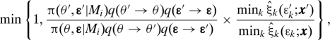and otherwise stay at (θ,ɛ,x), then return to ABCμ 1.

Please see Materials and Methods, section 4, for a technical discussion and Tables 1 and 2 for a comparison of the efficiency of ABCμ with related samplers.

Table 1.

Acceptance rate and average mixing quality in θ

Algorithm	B	acc.prob	Burn-in	${10}^3\frac{n_{\text{eff}}(\theta )}{n}$	$\frac{n_{\text{eff}}(\theta )}{\text{CPUhr}}$
ABC-MCMC (26)	1	0.002	105	0.7	13.4
Zoom-ABC-MCMC (12)	50/1	0.002	800	0.7	23.8
AUX-ABC (27)	1	0.01	105	0.6	4.5
ABCμ with asymmetric walk in ɛ, Eq. S12	50	0.36	771	25.6	24.6

Performance results are obtained from inference from the H. pylori PIN dataset; tuning parameters have been optimized for each algorithm separately (SI Appendix, S1.15). The effective sample size n_eff is taken as an indicator of mixing quality across n iterations (SI Appendix, S1.14). Importantly, n_eff(θ)/CPU hr must be compared relative to the achieved absolute errors (see further SI Appendix, Table S2). Higher acceptance rates are not necessarily desirable. As a rule of thumb, we found that, here, rates >0.45 reduced the effective sample size.

Table 2.

Mixing quality of the unknown error terms

Algorithm	B	103neff /n for ɛ of the summaries
		WR	DIA	CC	$\overline{\text{ND}}$	FRAG
AUX-ABC (27) with GRW in ɛ	1	0.1	0.23	0.13	0.07	0.05
ABCμ with GRW in ɛ	50	10.6	3.1	14.9	3.1	2.6
ABCμ with asymmetric walk in ɛ, Eq. S12	50	140	41.7	48.1	71.6	101

Mixing quality is quantified with the effective sample size n_eff for each error ɛ_k (ABC_μ) or random mismatch threshold (AUX-ABC), standardized per 1,000 iterations; tuning parameters have been optimized for each algorithm (SI Appendix, S1.15).

Model Criticism by Revealing Model Inconsistency Across Discrepancies.

For large datasets and/or complex models, the discrepancies ρ_k are often codependent (5, 17). Our approach to model criticism capitalizes on the fact that the co-dependencies among S_k(x) under the predictive distribution π(x|M_i) are typically different from those among S_k(x₀) if the model is not adequate, revealing model inconsistency in terms of conflicting, codependent summaries. As exemplified in Fig. 2, only a comprehensive set of summaries may enable model criticism; it is our view that choosing comprehensive summaries and discrepancy functions is crucial to ensure the approximation quality of Eq. 6 to the likelihood (12) as well as for model criticism based on posterior densities of summary errors (Eq. 7). To explore model adequacy, we recommend investigating various posterior quantities of f̂_ρ(ɛ|x₀, M_i) and using centrality measures such as high probability density (HPD) intervals; we remark at this point that marginal properties are in our setting typically not independent and caution against the overinterpretation of marginal diagnostics (see further Fig. 3).

Fig. 3.

Numerical estimates, obtained from ABCμ, of the approximate posterior error densities $\widehat{f}$_ρ(ɛ_k|x₀,M_i) combined with 50% box plots (black bars) for 2 of 7 summaries to quantify departures of 3 competing models of network evolution to the T. pallidum PIN dataset; PAPr employs sampling scheme RS1, whereas all others use sampling scheme RS2. ODBOX of PAPr is miniaturized by a factor of 5 to improve the visualization of differences across models for RS2. Whereas PAPr and PAP depart in ODBOX from the data, DD+LNK+PA departs (slightly) in $\overline{\text{ND}}$ from the observed PIN, suggesting that only DDA+PA provides an adequate fit the T. pallidum dataset.

Example: Criticizing Models of PIN Evolution

The structure of PINs derives from multiple stochastic processes over evolutionary timescales, and a number of mechanisms, based on randomly growing graphs, have been proposed to capture aspects of network growth (ref. 29 and references therein). We briefly motivate three models of network evolution. Recent comprehensive analyses across 181 prokaryotic genomes suggest that lateral gene transfer probably occurs at a low rate, but that, cumulatively, ≈80% of all genes in a prokaryotic genome are involved in lateral gene transfer (30); model PAP¶ is inspired by this scenario as it proposes network evolution in terms of attachment processes only (Materials and Methods, section 2). At least 40% of genes in prokaryotes appear to be products of gene duplication (31). Model DDA+PA (Materials and Methods, section 2) is designed to quantify the potential role of duplication and divergence in network evolution (12). At least for eukaryotes, the formation or degeneration of functional links between proteins (link turnover) is estimated to occur at a fast rate of ≈10⁻⁵ changed interactions per My per protein pair (20). We extend model DDA+PA into Model DD+LNK+PA (Materials and Methods, section 2), which includes link turnover in terms of preferential loss and gain of protein interactions. Crucially, ABC enables us to account for data incompleteness. Previously, we modeled missing data by randomly sampling proteins from the simulated data (RS1) (12). Here, we examine an alternative model that randomly samples from those proteins that have an interaction in the simulated data (RS2). (For the former, we add “r” to the model acronyms.) Necessarily, all models remain conceptually limited and must be cautiously interpreted; for example, the assumption that the network as a whole evolves at homogeneous rates has been questioned (32).

Models of Network Evolution Inspired by Horizontal Gene Transfer, Duplication-Divergence, and Link Turnover.

We ask whether the T. pallidum PIN topology is compatible with a number of fundamentally different modes of network evolution, in guise of simplified models. We successfully checked (Materials and Methods, section 5) and applied ABCμ (Materials and Methods, section 6) to sample from f̂_ρ(θ,ɛ|x₀,·) for the models PAP, DDA+PA, and DD+LNK+PA (under both sampling schemes RS1 and RS2); see Fig. 3 and SI Appendix, Figs. S5 and S6. Based on RS1 (12), all models depart significantly in FRAG as exemplified for PAPr in Table 3. This motivated us to consider alternative models of missing data, and we found no significant departures in FRAG for any of the considered evolution models under RS2; see Table 3. Turning to the 6 remaining discrepancy functions, we observe (Table 3 and Fig. 3), that only model DDA+PA matches the Treponema pallidum PIN adequately, suggesting that an evolutionary mode of duplication-divergence is most consistent with the T. pallidum PIN dataset. Repeating our analysis based on RS2 for the Helicobacter pylori PIN dataset, we could not substantiate our results further, because all considered models provide an adequate fit to the data. This is surprising, because we expect a similar power of our method on both datasets (SI Appendix, S1.19), and may point to qualitative differences among the two PINs owing to different, underlying experimental protocols.

Table 3.

Fifty percent high probability density intervals of ɛ_k |x₀, indicating model mismatch relative to the T. pallidum PIN

Mi	ɛCONN	ɛWR	ɛODBOX	ɛDIA	ɛCC	$\overline{\text{ND}}$	ɛFRAG
PAPr	[−0.11, 0.11]	[−0.11, 0.15]	[0.28, 0.72]	[−0.16, 0.92]	[−0.012,−0.002]	[−0.20, 0.05]	[0.08, 0.18]
PAP	[−0.15, 0.14]	[−0.12, 0.16]	[0.02, 0.61]	[−0.60, 0.91]	[−0.010,−0.003]	[−0.66, 0.01]	[−0.16, 0.01]
DDA+PA	[−0.24, 0.29]	[−0.34, 0.48]	[−0.12, 0.20]	[−0.48, 0.50]	[−0.002, 0.027]	[−0.66, 0.05]	[−0.01, 0.29]
DD+LNK+PA	[0.27, 0.21]	[−0.20, 0.17]	[−0.11, −0.55]	[−0.59, 0.32]	[−0.018,−0.006]	[−1.03,−0.16]	[0,0.11]

Note that the scales of ɛ_k correspond to the scales of the summaries, so that small numbers are meaningful. We caution against overinterpretation because the errors are not independent. See Materials and Methods, section 6, for further details.

Conclusion

The growing complexity of realistic models renders Bayesian model criticism increasingly important and difficult. In this article, we provide Bayesian techniques to comprehensively quantify discrepancies between the likelihood model and the data, simultaneously with parameter inference in situations when the likelihood is intractable, thus providing valuable guidance on the interpretability of parameter estimates and on how to improve models. We found this methodology helpful in iteratively identifying an adequate model of network evolution in terms of a large number of summaries; in particular, the PIN topology of the prokaryote T. pallidum provides little support for network evolution dominated by link turnover, or by lateral gene transfer alone. We close by cautioning that it is difficult to convincingly associate a formal framework to our high probability density intervals on multiple diagnostic error terms (6, 7). The presented methods will be useful in the initial stages of model and data exploration (16), and in particular, in efficiently scrutinizly several models by direct, inspection of their summary errors (5), prior to more formal analyses (14).

Materials and Methods

1. Summaries.

PINs can be described as graphs that contain a set of nodes, interacting proteins, and undirected binary edges, representing the observed interactions between the proteins. We consider the following topological summary statistics of PINs: Order, the number of nodes; size, the number of edges; node degree, the number of edges associated with a node; $\overline{\text{ND}}$, average node degree; distance, the minimum number of edges that have to be visited to reach a node j from node i; WR, within-reach distribution, the mean probability of how many nodes are reached from one node within distance k = 1,2,… (12); DIA, diameter, the longest minimum path among pairs of nodes in a connected component; CC, cluster coefficient, the mean probability that 2 neighbors of a node are themselves neighbours; BOX, the number of 4-cycles with 4 edges among the 4 nodes; FRAG, fragmentation, the percentage of nodes not in the largest connected component; CONN, log connectivity distribution, log(p(k₁,k₂)$\overline{\text{ND}}$²)/(k₁p(k₁)k₂p(k₂)), the depletion or enrichment of edges ending in nodes of degree k₁, k₂ relative to the uncorrelated network with same node degree distribution; ODBOX, BOX degree distribution, the probability distribution of BOXes with k edges to nodes outside the BOX. Examples are provided in SI Appendix, Table S1.

2. Algorithmic Details of the Models of Network Evolution.

Given a PIN x₀, we simulate a network under a given model to the number of genes in the respective genome, and account for incompleteness in x₀ by either RS1 or RS2. In model PAP evolution proceeds only by preferential attachment (33); at each step the number of attachments minus one is Poisson distributed with mean m. DDA+PA (12) features preferential attachment of a new node to one node of the existing network with probability α, or, with probability 1−α, a step of node duplication and immediate link divergence. In the latter case, a parent node is randomly chosen and its edges are duplicated. For each parental edge, the parental and duplicated one are then lost with probability δ_Div each, but not both; moreover, at least one link is retained to any node. The parent node may be attached to its child with probability δ_Att. DD+LNK+PA is a mixture of duplication-divergence (as above with parameter δ_Div but fixed δ_Att = 0), link addition and deletion, and preferential attachment as in DDA+PA. Link addition (deletion) proceeds by choosing a node randomly, and attaching it preferentially to another node (deleting it preferentially from its interaction partners) (20). At each step unnormalized weights are calculated as follows. For duplication-divergence, the rate κ_Dup is multiplied by the order of the current network; for link addition, the rate κ_LnkAdd is multiplied by $\left(\begin{array}{c}\text{Order}\\ 2\end{array}\right)$ − size; for link deletion, the unnormalized weight of link addition is multiplied by κ_LnkAdd. Preferential attachment occurs at a constant frequency α, and the weights of duplication, link addition, and link deletion are normalized so that their sum equals 1−α. Each of the components is chosen with these weights; the parameter ranges are determined by the prior (SI Appendix, S1.10).

3. Combining Multiple Error Terms.

It is difficult to compare ξ̂_k,θ,x0(ɛ_k) across k without further transformation, because summaries differ in their sensitivity to changes in θ (12) so that the scales of the density estimates vary across summaries and (to a lesser extent) across θ; see SI Appendix, Fig. S1. In Rejection-ABCμ (SI Appendix, S1.8), summaries may be precomputed and standardized, but this is not applicable in MCMC. We propose to standardize the variance of each ξ̂_k to one, bearing in mind that this might reduce approximation quality in some cases.

4. Details of ABCμ.

ABCμ is similar to the MCMC algorithm proposed in ref. 27; the latter also extends the state space, but includes a scalar τ (circumventing the need to design an efficient proposal q(ɛ → ɛ′)). We show that ABCμ eventually samples from f̂_ρ(θ,ɛx), provide convergence results for the smoothing approximation (SI Appendix, S1.5 and S1.11), discuss our non-standard proposal kernel (SI Appendix, S1.12), and provide final details (SI Appendix, S1.13). We do not claim that our smoothing approach based on repeated sampling from f(·|θ,M_i) comes at no cost. What we contend is that (i) we obtain improved mixing quality relative to ABC within MCMC, owing to a stabilized, numerical approximation of the likelihood with Eq. 9, and (ii) that we can construct more efficient proposal kernels, a point particularly relevant for ABCμ, where the number of error terms easily exceeds the dimensionality of θ. With respect to (i), we compared ABCμ with ABC-MCMC (26), zoomABC-MCMC (12), and AUX-ABC (27) on the H. pylori PIN dataset (SI Appendix, S1.15). Table 1 illustrates that ABCμ results in much improved acceptance rates and better mixing; this has already been suggested by Becquet and Przeworski (28) when f(s(x)|θ,M_i) is available in closed form. As for (ii), we devised a guided, asymmetric random walk in ɛ (SI Appendix, S1.12). This greatly improved both overall acceptance rate and mixing in ɛ compared to AUX-ABC and ABCμ with a (symmetric) Gaussian random walk (GRW) in ɛ (Table 2), exemplifying that effectively, repeated sampling may improve the efficiency of standard MCMC methods.

5. Testing ABCμ on PINs.

It was unclear whether our implementation is efficient enough to sample from Eq. 9. First, estimates of Eq. 7 might be inherently biased as for technically similar algorithms, and/or the PIN topology, in terms of the chosen summaries, might not be informative enough to evidence discrepancies between the model and the data. Second, given our smoothing approximation based on an adaptively chosen bandwidth h = h(x), we might be worried that posterior quantities of θ may be unreliable. We have addressed both concerns empirically (SI Appendix, S1.16), comforting that ABCμ provides useful numerical estimates of f̂_ρ(ɛ|x₀,M_i) to criticize the models of network evolution considered here, and suggesting that samples θ | x₀ from the marginal of Eq. 9, obtained by ABCμ, provide a good approximation to f_ρ(θ | x₀,M_i).

6. Criticizing Models of Network Evolution.

To contrast models PAP, DDA+PA, and DD+LNK+PA to the T. pallidum PIN dataset, ABCμ based on the summaries CONN, WR, ODBOX, DIA, CC, $\overline{\text{ND}}$, FRAG, and τ(ɛ|PAP) = (0.2,0.2,1.4,1,0.007,0.7,0.4), τ(ɛ|DDA + PA) = (1,0.7,0.8,0.5,0.05,0.5,0.4), and τ(ɛ|DD + LNK + PA) = (0.3,0.3,0.5,0.7,0.02,1.1,0.25) were used to generate 4 Markov chains as in SI Appendix, S1.15.

References

- 1.May RM. Uses and abuses of mathematics in biology. Science. 2004;303:790–793. doi: 10.1126/science.1094442. [DOI] [PubMed] [Google Scholar]
- 2.Box GEP. Science and statistics. J Am Stat Assoc. 1976;71:791–799. [Google Scholar]
- 3.Bernado JM, Smith AFM. Bayesian Theory. 1st Ed. Chichester, UK: Wiley & Sons; 1994. [Google Scholar]
- 4.Box GEP. Sampling and Bayes' inference in scientific modelling and robustness. J R Soc A (General) 1980;143:383–430. [Google Scholar]
- 5.Gelfand AE, Dey DK, Chang H. In: Bayesian Statistics 4. Bernardo JM, Berger JO, Dawid AP, Smith AFM, editors. Oxford: Oxford Univ Press; 1992. pp. 147–167. [Google Scholar]
- 6.Meng XL. Posterior predictive p-values. Ann Stat. 1994;22(3):1142–1160. [Google Scholar]
- 7.Bayarri MJ, Berger JO. In: Bayesian Statistics 6. Bernardo JM, Berger JO, Dawid AP, Smith AFM, editors. Oxford: Oxford Univ Press; 1999. pp. 53–82. [Google Scholar]
- 8.Liu JS. Monte Carlo Strategies in Scientific Computing. New York: Springer; 2001. p. 343. [Google Scholar]
- 9.Gouriéroux C, Monfort A. Simulation-Based Econometric Methods. Oxford: Oxford Univ Press; 1996. [Google Scholar]
- 10.Marjoram P, Tavaré S. Modern computational approaches for analysing molecular genetic variation data. Nat Rev Genet. 2006;7:759–770. doi: 10.1038/nrg1961. [DOI] [PubMed] [Google Scholar]
- 11.Riley S, et al. Transmission dynamics of the etiological agent of SARS in Hong Kong: Impact of public health interventions. Science. 2003;300:1961–1966. doi: 10.1126/science.1086478. [DOI] [PubMed] [Google Scholar]
- 12.Ratmann O, et al. Using likelihood-free inference to compare evolutionary dynamics of the protein networks of H.pylori and P.falciparum. PLoS Comp Biol. 2007;3:e230. doi: 10.1371/journal.pcbi.0030230. [DOI] [PMC free article] [PubMed] [Google Scholar]
- 13.Wilkinson RD. Bayesian inference of primate divergence times. Cambridge: Univ of Cambridge; 2007. PhD thesis. [Google Scholar]
- 14.Fagundes NJR, et al. Statistical evaluation of alternative models of human evolution. Proc Natl Acad Sci USA. 2007;104:17614–17619. doi: 10.1073/pnas.0708280104. [DOI] [PMC free article] [PubMed] [Google Scholar]
- 15.Toni T, Welch D, Strelkowa N, Ipsen A, Stumpf MPH. Approximate Bayesian computation scheme for parameter inference and model selection in dynamical systems. J R Soc Interf. 2008 doi: 10.1098/rsif.2008.0172. 10.1098rsif. 2008.0172. [DOI] [PMC free article] [PubMed] [Google Scholar]
- 16.Zellner A. Bayesian analysis of regression error terms. J Am Stat Assoc. 1975;70:138–144. [Google Scholar]
- 17.O'Hagan A. In: Highly Structured Stochastic Systems. Green PJ, Hjort NL, Richardson S, editors. Oxford: Oxford Univ Press; 2003. pp. 423–453. [Google Scholar]
- 18.Rain JC, et al. The protein-protein interaction map of Helicobacter pylori. Nature. 2001;409:211–215. doi: 10.1038/35051615. [DOI] [PubMed] [Google Scholar]
- 19.Titz B, et al. The binary protein interactome of Treponema pallidum—The Syphilis spirochete. PLoS ONE. 2008;3:e2292. doi: 10.1371/journal.pone.0002292. [DOI] [PMC free article] [PubMed] [Google Scholar]
- 20.Beltrao P, Serrano L. Specificity and evolvability in eukaryotic protein interaction networks. PLoS Comp Biol. 2007;3:e25. doi: 10.1371/journal.pcbi.0030025. [DOI] [PMC free article] [PubMed] [Google Scholar]
- 21.Pinney JW, Amoutzias GD, Rattray M, Robertson DL. Reconstruction of ancestral protein interaction networks for the bZIP transcription factors. Proc Natl Acad Sci USA. 2007;104:20449–20453. doi: 10.1073/pnas.0706339104. [DOI] [PMC free article] [PubMed] [Google Scholar]
- 22.Hakes L, Pinney JW, Robertson DL, Lovell SC. Protein-protein interaction networks and biology—What's the connection? Nat Biotechnol. 2008;26:69–72. doi: 10.1038/nbt0108-69. [DOI] [PubMed] [Google Scholar]
- 23.Wilkinson RD. Approximate Bayesian Computation (ABC) gives exact results under the assumption of model error. 2008 doi: 10.1515/sagmb-2013-0010. arXiv:0811.3355v1 [stat.CO] [DOI] [PubMed] [Google Scholar]
- 24.Sisson SA, Fan Y, Tanaka MM. Sequential Monte Carlo without likelihoods. Proc Natl Acad Sci USA. 2007;104:1760–1765. doi: 10.1073/pnas.0607208104. [DOI] [PMC free article] [PubMed] [Google Scholar]
- 25.Gilks WR, Richardson S, Spiegelhalter DJ. Markov Chain Monte Carlo in Practice. London: Chapman & Hall; 1996. [Google Scholar]
- 26.Marjoram P, Molitor J, Plagnol V, Tavaré S. Markov Chain Monte Carlo without likelihoods. Proc Natl Acad Sci USA. 2003;100:15324–15328. doi: 10.1073/pnas.0306899100. [DOI] [PMC free article] [PubMed] [Google Scholar]
- 27.Bortot P, Coles S, Sisson S. Inference for stereological extremes. J Am Stat Assoc. 2007;102:84–92. [Google Scholar]
- 28.Becquet C, Przeworski M. A new approach to estimate parameters of speciation models with application to apes. Genome Res. 2007;17:1505–1519. doi: 10.1101/gr.6409707. [DOI] [PMC free article] [PubMed] [Google Scholar]
- 29.Knudsen M, Wiuf C. A Markov chain approach to randomly grown graphs. J Appl Math. 2008 10.1155/2008/190836. [Google Scholar]
- 30.Dagan T, Artzy-Randrup Y, Martin W. Modular networks and cumulative impact of lateral transfer in prokaryote genome evolution. Proc Natl Acad Sci USA. 2008;105:10039–10044. doi: 10.1073/pnas.0800679105. [DOI] [PMC free article] [PubMed] [Google Scholar]
- 31.Chothia C, Gough J, Vogel C, Teichmann SA. Evolution of the protein repertoire. Science. 2003;300:1701–1703. doi: 10.1126/science.1085371. [DOI] [PubMed] [Google Scholar]
- 32.Davidson EH, Erwin DH. Gene regulatory networks and the evolution of animal body plans. Science. 2006;311:796–800. doi: 10.1126/science.1113832. [DOI] [PubMed] [Google Scholar]
- 33.Barabási A, Albert R. Emergence of scaling in random networks. Science. 1999;286:509–512. doi: 10.1126/science.286.5439.509. [DOI] [PubMed] [Google Scholar]
Associated Data
This section collects any data citations, data availability statements, or supplementary materials included in this article.