Figure-ground interaction in the human visual cortex

Abstract

Discontinuities in feature maps serve as important cues for the location of object boundaries. Here we used multi-input nonlinear analysis methods and EEG source imaging to assess the role of several different boundary cues in visual scene segmentation. Synthetic figure/ground displays portraying a circular figure region were defined solely by differences in the temporal frequency of the figure and background regions in the limiting case and by the addition of orientation or relative alignment cues in other cases. The use of distinct temporal frequencies made it possible to separately record responses arising from each region and to characterize the nature of nonlinear interactions between the two regions as measured in a set of retinotopically and functionally defined cortical areas. Figure/background interactions were prominent in retinotopic areas, and in an extra-striate region lying dorsal and anterior to area MT+. Figure/background interaction was greatly diminished by the elimination of orientation cues, the introduction of small gaps between the two regions, or by the presence of a constant second-order border between regions. Nonlinear figure/background interactions therefore carry spatially precise, time-locked information about the continuity/discontinuity of oriented texture fields. This information is widely distributed throughout occipital areas, including areas that do not display strong retinotopy.

Introduction

The segmentation of objects from their backgrounds is believed to involve a combination of border and surface processing operations. Object borders produce discontinuities in image features such as orientation, spatial texture, color, depth, collinearity, or motion. By comparison, object surfaces and support structures, such as the background, typically comprise regions where these properties vary more slowly. Not surprisingly, the processing of both image discontinuities and the grouping of features over space have featured prominently in models of image segmentation (Grossberg & Mingolla, 1985; Koechlin, Anton, & Burnod, 1999; Li, 2000; Malik & Perona, 1990; Roelfsema, Lamme, Spekreijse, & Bosch, 2002; Thielscher & Neumann, 2003) and in empirical studies (Bach & Meigen, 1992; Lamme, Van Dijk, & Spekreijse, 1992; Landy & Bergen, 1991; Marcus & Van Essen, 2002; Nothdurft, 1991; Song & Baker, 2006; Sutter & Graham, 1995).

We have previously shown that the figure and background regions of figure/ground displays activate distinct cortical networks (Appelbaum, Wade, Vildavski, Pettet, & Norcia, 2006). In that study, the figure region was temporally modulated at one frequency and the background region at another allowing us to use spectral analysis to separate the responses from the two simultaneously presented regions. We found that regions of visual space, that are consistent with a figure occluding a background texture, were preferentially processed by a network of lateral and ventral visual areas that have been previously associated with the processing of objects (Grill-Spector, Kushnir, Edelman, Itzchak, & Malach, 1998; Marcar et al., 2004; Vuilleumier, Henson, Driver, & Dolan, 2002). The background region, in contrast, elicited activity from first-tier and more dorsal cortical areas.

Our measurements were based on an analysis of the distinct harmonics associated with the figure and background temporal frequencies. Previous studies (Hou, Pettet, Sampath, Candy, & Norcia, 2003; Norcia, Wesemann, & Manny, 1999; Victor & Conte, 2000; Zemon & Ratliff, 1984) have also used the temporal tagging method to study nonlinear spatio-temporal interactions between regions. The analysis of EEG responses in a two-frequency experiment allows one to separate responses from three logically distinct populations of cells, as illustrated in Figure 1. In the illustration, the figure region (indicated by horizontal texture) is temporally modulated at one frequency (f₁) and the background (indicated by vertical texture) is modulated at a different frequency (f₂). Neurons with restricted receptive fields that lie entirely within the figure region (magenta) will “see” f₁ on their inputs and will generate responses at frequencies that are harmonics of f₁. Neurons whose receptive fields lie entirely within the background regions (cyan) will have f₂ on their inputs and will generate responses at harmonics of f₂. Similarly restricted receptive fields that span the two regions (yellow, left panel) may have harmonics of f₁ and f₂ as well as frequencies equal to low-order sums and differences of f₁ and f₂ on their outputs if the stimulus configuration matches their receptive field, and if they have an output nonlinearity, such as a firing threshold. By itself, the analysis cannot distinguish small receptive field that span the border from very large receptive fields that cover both regions (yellow right panel). However, by varying the image structure, it is possible to study the stimulus preferences of the three classes of cells.

Figure 1.

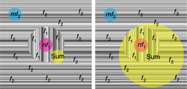
Schematic illustration of hypothetical populations of neurons responding to a texture segmentation display. The figure region is driven at a frequency equal to f₁ and the background is driven at a frequency equal to f₂. Neurons with receptive fields that are restricted to the figure region (magenta) generate responses at harmonics of f₁ (nf₁). Neurons with receptive fields that are restricted to the background region (cyan) generate responses at harmonics of f₂ (mf₂). Neurons whose receptive fields span both regions (yellow) may generate responses at both nf₁ and mf₂, as well as frequencies equal to nf₁ ± mf₂, where n and m are small integers (e.g., the sum 1f₁ + 1f₂).

Here we use two-region displays that are spatially asymmetric: a small figure region surrounded by a large background to study how figure-ground interaction depends on the orientation structure of the textures that are used to define the regions. To test the relative importance of the texture discontinuities at the figure/background border, we varied the separation between figure and background regions and presented stimuli with a constant second-order border between regions, therefore controlling for the global segmentation of the stimuli. We found that border-related signals occur in both first-tier visual areas and in a nonretinotopic region of extra-striate cortex that lies dorsal and anterior to the site of maximal figure region response.

Materials and methods

Participants

A total of 13 observers participated in these experiments (mean age 33). All participants had visual acuity of better than 6/6 in each eye, with correction if needed, and stereoacuity of 40 arc seconds or better on the Titmus and Randot stereoacuity tests. Acuity was measured using the Bailey-Lovie chart, which has five letters per line and equal log increments in the letter sizes across lines. Informed consent was obtained prior to experimentation under a protocol that was approved by the Institutional Review Board of the California Pacific Medical Center.

Stimulus construction and frequency tagging procedure

Stimulus generation and signal analysis were performed by in-house software, running on a Macintosh G4 platform. Stimuli were presented in a dark and quiet room on a Sony multi-synch video monitor (GDP-400) at a resolution of 800 χ 600 pixels, with a 72-Hz vertical refresh rate. The nonlinear voltage versus luminance response of the monitor was corrected in software after calibration of the display with an in-house linear PIN-diode photometer equipped with a photopic filter. Participants were instructed to fixate a cross at the center of the display and to distribute attention evenly over the entire display. Individual trials lasted 16.7 seconds and stimulus conditions were randomized within a block. A typical session lasted roughly an hour and consisted of 10-20 blocks of randomized trials in which the observer paced the presentation and was given opportunity to rest between blocks.

The stimuli presented in these experiments included the stimuli utilized in (Appelbaum et al., 2006) as well as several additional variations. Eight different stimulus conditions were presented in a single session for the first experiment and 7 additional conditions were presented in a second session. Eight of the thirteen observers who participated in the first session also participated in the second session. Animations of all stimuli are provided in the Supplementary materials.

Disk-on-background configurations defined by different cues (13 observers)

In this session, figure and background regions were defined on the basis of differences in orientation, relative alignment, contrast, and/or temporal frequency. Data from several of these conditions were presented in (Appelbaum et al., 2006). In one condition, the “phase-defined form” stimulus (Figure 2A, left panel), a 5° circular figure region was defined by local contrast discontinuities at the border of horizontally oriented figure and background textures. The textures comprising both figure and background regions consisted of one-dimensional random-luminance bars. The minimum bar width was 6 arcmin and the maximum contrast between elements was 80%, based on the Michelson definition. The figure region rotated by 180° at 3.0 Hz (f₁), and the background region (a 20° square texture field) was rotated at 3.6 Hz (f₂). Because the figure region was composed of the same texture as the background region, it either blended seamlessly into the background when both figure and background were in their unrotated state or appeared to be segmented from the background when the rotation state of either the figure or background differed (see four stimulus frames). Since the orientation of the figure and background regions was always horizontal, the segmentation was defined by spatio-temporal luminance discontinuities along the length of the bars that occurred at the figure/background border.

Figure 2.

Stimulus schematics illustrating four stimulus frames for each of four cue types; (A) phase-defined, (B) orientation-defined, (C) temporally-defined, and (D) luminance/texture defined. Comparison stimuli in which the segmentation state is constant are shown on the right for the phase-defined stimulus. The temporal structure and resulting segmentation states of the two-frequency stimuli is illustrated below E).

An `orientation-defined form' stimulus (Figure 2B) was generated by rotating the figure and background regions by 90° rather than 180°. The figure region segmented from the background whenever the rotation state of the two regions differed, as in the phase-defined form, but in this case there was a 90° orientation difference between the two regions in the segmented state. By using square random-luminance elements (6 arcmin on a side), orientation information was removed altogether, forcing the segmentation process to rely solely on the two different temporal tags. In these `temporally defined form' stimuli (Figure 2C), no orientation information exists and segmentation information is presumably carried by the detection of temporal asynchrony between the two regions.

In addition to the stimuli already described, one stimulus condition containing only a single frequency tag was included to assess the responses to the figure alone in the absence of a background texture and the segmentation appearance and disappearance resulting from their interactions. In the `figure only' condition, the figure region was presented on a mean gray background containing no texture. In this stimulus, the figure alternated orientation by 90- at 3.0 Hz. The figure size and shape was the same as in the other conditions, but here the figure segmentation is continuous and defined by a difference in contrast (0% vs. 80%) and temporal frequency (0 vs. 3.0 Hz).

Because the global figure-ground configuration of these stimuli alternated between a uniform field and a segmented one, we refer to these conditions as `changing segmentation' conditions. Variants of the phase- and orientation-defined forms in which the texture in the figure region did not match that of the background were also presented. In these stimuli, the figure and background regions were composed of different random luminance textures, and therefore the figure never blended into the background. In these stimuli (Figure 2A, right), referred to as `constantly segmented,' a border was always present between regions, and there was never a uniform state. This manipulation was designed to isolate aspects of processing that were specific the appearance and disappearance of the segmented form, or alternatively the importance of continuous, collinear texture. The mean luminance of all stimuli was 56.3 cd/m², and the full display subtended 20° by 20° of visual angle.

A schematic representation of the temporal structure of figure segmentation over one full stimulus cycle (1.67 sec) is illustrated in Figure 2D. In this illustration, the states of the background (top square wave) and the figure (bottom square wave) are depicted by the solid lines. The sequence of figure segmentation resulting from these modulations is indicated by the shaded gray (segmented) and white (unsegmented) areas.

Spatial separation (gap) variations (8 observers)

In a separate experimental session, a centrally presented, 3°, phase-defined form was used to test the effects of the local structure of the border region on the driven EEG response. The figure and background regions were either contiguous, had a mean luminance gap between regions (Figure 2A, right), or were continuously segmented (as described above, Figure 2A, center). The five gaps sizes were 5′,10′,15′,20′, and 60′ (1°) of visual angle. The figure was always 3° and the background always extended 7.6° × 7.6°. Viewing distance was 200 cm.

EEG signal acquisition and source imaging procedure

The analytical procedures for this experiment (EEG signal acquisition, head conductivity modeling, source estimation, visual areas definition, region-of-interest quantification, and statistical analysis) are similar to those described in Appelbaum et al. (2006). In the interest of brevity, we will only provide an overview of these methods here.

EEG signal acquisition

The electroencephalogram (EEG) was collected with 128-sensor HydroCell Sensor Nets (Electrical Geodesics, Eugene OR) that utilize silver-silver chloride electrodes embedded in electrolyte soaked sponges. The EEG was amplified at a gain of 1,000 and recorded with a vertex physical reference. Signals were 0.1 Hz high-pass and 200 Hz (elliptical) low-pass filtered and digitized at 432 Hz with a precision of 4-bits per microvolt at the input. Following each experimental session, the 3D locations of all electrodes and three major fiducials (nasion, left and right peri-auricular points) were digitized using a 3Space Fastrack 3-D digitizer (Polhemus, Colchester, VT). For all observers, the 3D digitized locations were used to co-register the electrodes to their T1-weighted anatomical Magnetic Resonance (MR) scans.

Artifact rejection and spectral analysis of the EEG data were done off-line. Raw data were evaluated according to a sample-by-sample thresholding procedure to remove noisy sensors that were replaced by the average of the six nearest spatial neighbors. Once noisy sensors were substituted, the EEG was re-referenced to the common average of all the sensors. Additionally, EEG epochs that contained a large percentage of data samples exceeding threshold (~25-50 microvolts) were excluded on a sensor-by-sensor basis. Time averages for each stimulus condition were computed over one stimulus cycle (1.67 sec). The time averages were then converted to complex-valued amplitude spectra at a frequency resolution of 0.6 Hz via a discrete Fourier transform. The resulting amplitude spectra of the steady-state visually evoked potential (SSVEP) were then evaluated at a set of frequencies uniquely attributable to the input stimulus frequency tags up to the 18th and 15th harmonic for the figure and background tags, respectively. Preliminary analysis of the statistical significance of individual observer data was conducted using the T_circ² methods described by (Victor & Mast, 1991).

Spectral analysis of the EEG

Periodic visual stimulation leads to a periodic visual response that occurs at frequencies equal to exact integer multiples of the stimulation frequency (Regan, 1989). Due to the nonlinear nature of visual cortical processing, responses are observed at frequencies that are not present in the input (Baitch & Levi, 1988; Burton, 1973; Candy, Skoczenski, & Norcia, 2001; Regan & Regan, 1987).

As an illustration, consider a simple squaring nonlinearity. Passing two sinusoidally modulating inputs, one of frequency f₁ and amplitude A and the other of frequency f₂ and amplitude B, through this nonlinearity yields the following output spectrum:

$$\begin{array}{cc}\hfill {(A\cos 2\pi f_{1}t+B\cos 2\pi f_{2}t)}^2& =(A^2∕2)(1+\cos 2\pi 2f_{1}t)\hfill \\ \hfill & +(B^2∕2)(1+\cos 2\pi 2f_{2}t)\hfill \\ \hfill & +AB\cos 2\pi (f_1-f_2)t\hfill \\ \hfill & +AB\cos 2\pi (f_1+f_2)t.\hfill \end{array}$$ (1)

The output of this nonlinearity contains new frequencies, at 2f₁,2f₂, f₁ - f₂, and f₁ + f₂, with 2f₁ and 2f₂ being the second harmonics of the two stimulus frequencies and f₁ - f₂ and f₁ + f₂ being the difference and sum intermodulation frequencies, respectively. These intermodulation frequencies reflect temporal interactions between the two inputs and are therefore referred to as `interaction terms' or `mutual terms,' whereas the harmonics of the input frequencies reflect interactions between each tag and itself and are known as the `self-terms.'

The particular self-terms and interaction terms produced and their magnitudes depend on the specific form of the nonlinearity and the number of frequency components in the input. By carefully choosing the temporal frequencies of multi-input stimuli, one can arrange that the self-terms associated with each input and the mutual terms that result from their interaction occur at unique frequencies in the response spectrum and therefore can be separated from one another by appropriate scrutiny of the response spectrum. Frequency pairs that have the property of sharing no common multiples or low-order sum and difference frequencies are said to be incommensurate (Victor & Shapley, 1980).

The stimulus frequencies in our experiments were chosen so that corresponding periods each consisted of an integer number of video frames (24 frames for the 3-Hz stimulus and 20 frames for the 3.6-Hz stimulus for the frame rate of 72 Hz). For this pair of frequencies, all possible self- and mutual terms are integer multiples of the 0.6-Hz difference frequency, and we thus averaged raw data over a 1.667-second interval and performed Fourier analysis at 0.6-Hz resolution. The use of frequencies whose periods are discrete submultiples of a relative small integer (e.g., 72) leads to some overlapping response components. The first 8 harmonics of each input are all distinct, except for the 6th harmonic of 3 Hz and the 5th harmonic of 3.6 Hz. The mutual terms, up to fourth-order, are also distinct from one-another and from the self-terms.

When temporal square waves are used, the inputs contain higher odd-harmonic components (e.g., the 3.0-Hz input has third harmonic temporal contrast equal to one-third that of the fundamental, and fifth-harmonic contrast equal to one-fifth of the fundamental, etc.). This introduces some additional complication that must be considered. For example, the second harmonic of 3.6 Hz (1f₂) shares the 7.2-Hz frequency bin with the fourth-order mutual term 2f₁ - 1f₂ of the respective third harmonics, where 3f₁ is 9 Hz and 3f₂ is 10.8 Hz. However, the dominant nonlinear interaction terms in our experiments (the second- and fourth-order sum frequencies) are distinct.

Spectral components of the evoked response are complex valued; i.e., they have both amplitude and phase, and can be plotted in a two-dimensional complex Cartesian coordinate system. A given spectral component for the group of observers can therefore be treated as a random variable, sampled from a bi-variate normal distribution. The error statistics for this distribution can thus be computed from the variance present in two distributions. Specifically, for the 2D plots in Figure 7 and Supplementary Figures 2 and 3, we treated the complex-valued samples as 2D vectors and then computed the principal axes of dispersion by eigen decomposition of the resulting covariance matrix (Johnson & Wichern, 1998). In Figure 7 and Supplementary Figure 3, the dispersion ellipses represent the 95% confidence interval of the mean using the square root of the covariance axes scaled by the constant, 2(n - 1)/(n(n - 2)) * F^-1(0.95, 2, n - 2), where n is the number of subjects, and F^-1 is the inverse of the cumulative F-distribution. In Supplementary Figure 2, the dispersion ellipses represented the standard error of the mean, using the normalization constant 1/(n - 2).

Figure 7.

Spectral phase distributions: Cortical phase maps and 2-D complex-valued ROI responses are shown at four frequencies for the phase-defined form stimulus. Unthresholded grand average phase maps are shown from posterior and lateral perspectives (left) next to the mean thresholded (1/3 max) amplitude maps from Figure 4 (right). Average ROI responses for V1, V2d, V3d, V3A, V4, LOC, MT+, and TOPJ are shown below their corresponding maps. Ellipses indicate 95% confidence limits and the phase convention places 0- delay at 3o'clock, as indicated by the color wheel.

Head conductivity and geometry models

As part of the source-estimation procedure, head tissue conductivity models were derived for 9 of the 13 individuals from T1-weighted MR scans. Boundary element models were computed based on compartmentalized tissue segmentations that defined contiguous regions for the scalp, outer skull, inner skull, and the cortex. To begin, approximate cortical tissue volumes for gray and white matter were defined by voxel intensity thresholding and anisotropic smoothing using the EMSE package (Source Signal Imaging, San Diego, CA, http://www.sourcesignal.com/). The resulting white matter tissue boundaries were used to extract the contiguous cortical gray matter surface. Using the cortical gray matter, an expansion algorithm was then run to derive the inner and outer surfaces of the skull. The scalp surface was then determined by removing extraneous extra-scalp noise and defining the surface with a minimum imposed thickness. Because the precise shape of the cortex is critical in determining the orientation of the cortical sources, we replaced the rapid cortical segmentation produced by EMSE with a more accurate segmentation of the cortical pial surface generated with the FreeSurfer software package (http://surfer.nmr.mgh.harvard.edu).

Finally, the scalp, skull, and brain regions were bounded by surface tessellations and all tissue surface tessellations were visually checked for accuracy to assure that no intersection had occurred between concentric meshes. Co-registration of the electrode positions to the MRI head surface was done by alignment of the three digitized fiducial points with their visible locations on the anatomical MRI head surface using the Locator module of the EMSE Suite. Final adjustments were completed using a least squares fit algorithm and electrode deviations from the scalp surface were removed.

Cortically constrained minimum norm source estimates

Estimates of the underlying cortical activity based on measurements of the potential recorded at the scalp were derived using the cortically constrained Minimum Norm estimate of the EMSE package. This technique assumes that surface EEG signals are generated by multiple dipolar sources that are located in the gray matter and oriented perpendicular to the cortical surface. Cortical current density (CCD) estimates were determined based on an iterative approach that attempts to produce a continuous map of current density on the cortical surface having the least total (RMS) power while still being consistent with the voltage distribution on the scalp. In addition, the EMSE implementation uses lead-field normalization to compensate the inherent bias toward superficial sources of the unweighted minimum norm inverse (Lin et al., 2006). For visualization purposes, current density distributions were computed from multi-subject electrode averages (sensor-space average). These average estimates are displayed on one individual's cortical surface (e.g., Figure 4). For descriptive purposes, we refer to current density (pA/mm²) as the source response magnitude and the sensor voltages as response amplitude.

Figure 4.

Average voltage and current distributions are shown at the second harmonic of each tag frequency (rows 1 and 2) and at their 2nd and 4th order sums (rows 3 and 4). For each response, average spline interpolated topographic maps (μV) and cortical surface current density distributions (three views, thresholded at 1/3 the max in pA/mm²) are shown with their corresponding maximum scale values (see colorbars below). Second harmonic responses for the figure (row 1) and background (row 2) show distinct distributions that are similar across cue types. Second-order sum-term interaction is large (row 3) for phase- and orientation-defined forms but not for temporally defined forms (note scale values). The magnitude and distribution of the fourth-order interaction (row 4) also differs somewhat across cue type.

Visual area definition by fMRI functional and retinotopic mapping

For all observers, functional magnetic resonance imaging (fMRI) scans were collected on very similar 3T GE scanners located at either the Stanford Lucas Center or the UCSF China Basin Radiology Center. Data from Stanford were acquired with a custom whole-head 2-channel coil or a 2-channel posterior head surface coil and a spiral K-space sampling pulse sequence. At UCSF, a standard GE 8-channel head-coil was used together with an EPI sequence. Despite slight differences in hardware and pulse sequence, the data quality from the two sites was very similar. The general procedures for these scans (head stabilization, visual display system, etc.) are standard and have been described in detail elsewhere (Brewer, Liu, Wade, & Wandell, 2005; Likova & Tyler, 2005). Retinotopic field mapping produced regions-of-interest (ROIs) defined for each participant's visual cortical areas V1, V2v, V2d, V3v, V3d, V3A, and V4 in each hemisphere (DeYoe et al., 1996; Tootell & Hadjikhani, 2001; Wade, Brewer, Rieger, & Wandell, 2002). ROIs corresponding to each participant's hMT+ were identified using low contrast motion stimuli similar to those described by Huk, Dougherty, and Heeger (2002).

The lateral occipital complex (LOC) was defined in one of two ways. For four participants, the LOC was identified using a block-design fMRI localizer scan. During this scan, the observers viewed blocks of images depicting common objects (18 s/block) alternating with blocks containing scrambled versions of the same objects. The stimuli were those used in a previous study (Kourtzi & Kanwisher, 2000). The regions activated by these scans included an area lying between the V1/V2/V3 foveal confluence and hMT+ that we identified as LOC.

The LOC is bounded by retinotopic visual areas and area hMT+. For observers without a LOC localizer, we defined the LOC on flatted representations of visual cortex as a polygonal area with vertices just anterior to the V1/V2/V3 foveal confluence, just posterior to area hMT+, just ventral to area V3B, and just dorsal to area V4. This definition covers almost all regions (e.g., V4d, LOc, LOp) that have previously been identified as lying within object-responsive lateral occipital cortex (Kourtzi & Kanwisher, 2000; Malach et al., 1995; Tootell & Hadjikhani, 2001) and none of the `first-tier' retinotopic visual areas. No qualitative differences were observed in the responses for the two methods of LOC ROI definition in our previous study (Appelbaum et al., 2006). See Supplementary materials, Section 2 for more details.

For all participants, additional activity was observed outside of retinotopic or functionally defined cortex, as defined from the fMRI methods detailed above. Systematic responses, prominent at the sum term (1f₁ + 1f₂), prompted the definition of an additional ROI in an extra-striate region lying dorsal and anterior to area MT+. Definition of this ROI was done on flattened cortical representations on a hemisphere-by-hemisphere and observer-by-observer basis. Data from the phase-defined form condition were used. ROI boundaries were hand drawn to encompass secondary maxima whose magnitudes were ~>1/3 of the maximum response that were not already accounted for by the other ROI. As described in the Results, consistent with the anatomical location of this ROI, we refer to it as the temporal-occipital-parietal junction (TOPJ).

Region-of-interest (ROI) response quantification

In order to avoid inaccuracies associated with individual differences in cortical geometry with respect to the sensors and the precise location of visual areas with respect to gyri and sulci, we extracted evoked response data from CCD distributions that lay within specific retinotopically or functionally defined regions-of-interest on a subject-by-subject basis. ROI-based analysis of the EEG data was performed by extending the Stanford VISTA toolbox (http://white.stanford.edu/software/) to accept EMSE-derived minimum norm inverses that were in turn combined with the cycle-averaged EEG time courses to obtain cortical current density distributions over the cortex mesh. An estimate of the tagged response for each ROI was computed as follows: First, the complex-valued Fourier components for each unique response frequency were computed for each mesh vertex using a discrete Fourier transform. The transform was computed over a 1.667-second epoch that contained an exact integer number of response cycles at each frequency of interest and an integer number of samples per cycle. Next, a single complex-valued component was computed for each ROI by averaging across all nodes within that ROI (typically >300). This averaging was performed on the complex Fourier components and therefore preserved phase information. Averaging across hemispheres and observers was then performed coherently for each individual frequency component (see Figure 5 for example of resulting histograms). The statistical significance of the harmonic components of each observer's single condition data was evaluated using the T_circ² statistic (Victor & Mast, 1991). This statistic utilizes both amplitude and phase consistency across trials to asses whether stimulus-locked activity is present.

Figure 5.

ROI response histograms are shown for the second-(left) and fourth-order (right) sum terms. Average projected magnitudes and standard errors are plotted for each ROI. Separate ROIs are color-coded as indicated in the legend at the bottom. The locations of these ROIs are shown for a single observer from 5 perspectives. Noise estimates are derived from the figure only condition (bottom row) and shown as black lines overlaid on the ROI response profile for all other conditions. Scales are indicated in the bottom plot.

Multivariate analysis of variance (MANOVA)

Differences between experimental design factors of response component (2f₁,2f₂,1f₁ +1f₂,2f₁ +2f₂), cue (phase-, orientation-, and temporally-defined form), configuration (changing or constantly segmented), and gap size (0′,5′,10′,15′,20′, and 60′) were assessed using a multivariate approach to repeated measures (multivariate analysis of variance; MANOVA) that, unlike univariate ANOVA, takes into account the correlated nature of repeated measures (for a review, see Keselman, Algina, & Kowalchuk, 2001). The specific design factors and levels are described in the appropriate section in the Results.

Standard MANOVA techniques are designed for use with scalar-valued quantities and they thus discard information about the phase-consistency of responses between observers. Without phase, highly coherent responses between observers become indistinguishable from incoherent responses. To address this issue, we devised a measure of response amplitude that preserves some of this phase information. We began by computing the mean complex-valued response vector across observers, and then projected each observer's complex-valued response onto this mean response vector. The amplitudes of these projected response vectors were used for MANOVA. The complex-valued responses of the subjects follow an elliptical, bivariate normal distribution around their mean, and the amplitudes of the projected responses follow a univariate normal distribution around the mean projected amplitude. for a small signal with a given level of additive noise, phases will be roughly consistent across observers, and the mean of unprojected amplitudes will roughly agree with the mean of the projected amplitudes. However, when the signal is absent and the phases are random across observers, the expected mean of the unprojected amplitudes will tend to stay the same, while the expected mean of the projected amplitudes will tend toward zero. This expectation of zero mean in the absence of coherent signal boosts the sensitivity of the MANOVA and better conforms to its distributional assumptions. Unless otherwise stated, all histogram and line-chart values indicate mean projected amplitudes ±SEM across observers.

Results

Separating region-derived components and their interaction

Statistically significant steady-state-evoked responses were present at harmonics of the distinct region-tag frequencies in all stimulus conditions and for all observers, but the magnitude and presence of the inter-region interaction terms, particularly the 1f₁ +1f₂ term, depended on stimulus condition and border arrangement. figure 3A shows the temporal frequency spectrum for the phase-defined form stimulus as an overlay of all 128 locations for the 13-observer sensor-space average. Prominent responses are visible at the harmonics of the region tag frequencies (2f₁,2f₂,4f₁,4f₂, etc.), with the amplitude of these responses (and the background EEG noise) decreasing with increasing frequency. The second harmonics (2f₁; 6.0 and 2f₂; 7.2 Hz) are the dominant region-response components. Since the image updating procedure produces two temporal transients for each cycle, it is not surprising that a large response would be evoked at the second harmonic. The observation that the responses are dominated by even harmonics of the tag frequencies indicates that each stimulus transition evoked similar responses in the population.

Figure 3.

EEG spectra derived from the phase-defined form are shown for (A) the 13 observer average with all 128 sensors superimposed and (B) for a single sensor from one observer. Figure responses are indicted in blue, background responses in cyan, and nonlinear interactions in red.

The individual observer, single sensor spectrum in Figure 3B, illustrates the smaller region interaction components in relationship to the region responses. The responses evoked by the figure region are shown in dark blue (nf₁), while those evoked by the background are shown in light blue (nf₂). Responses that reflect nonlinear interaction between regions (e.g., the mutualor intermodualtion terms) occurred at frequencies equal to low-order sums and differences of the two tags and are highlighted in red (nIM, where IM stands for intermodulation). Those frequency components colored in gray did not meet the statistical criterion of p > 0.05 (T²_circ test). This single sensor spectrum illustrates the presence of multiple, statistically significant interaction terms, with the largest coupling occurring at the sum frequency (1f₁ +1f₂; 6.6 Hz).

There are many possible frequencies at which nonlinear figure/ground interactions could occur (e.g., all frequencies equal to nf₁ + mf₂, where n and m are integers). In practice, only small integer combinations are observed, and among these only responses with even parity (e.g., m and n are both 1, or both even) are substantial. Tags at f₁ and f₂ were chosen to be close together so as to minimize the effects that differences in temporal frequency might have on region processes, and we have shown previously (Appelbaum et al., 2006) that the pattern of region responses did not depend on the whether the 3.0- or 3.6-Hz tag was applied to the figure or the background. This experimental design choice however has the consequence that second- and fourth-order difference frequencies (1f₂ — 1f₁; 0.6 Hz and 2f₂ — 2f₁; 1.2 Hz) are located in an unfavorable part of the EEG spectrum where spontaneous EEG activity (noise) is high. In order to determine which interaction terms could be used for further analysis, we first determined which of these frequencies evoked responses that could be observed above the spontaneous EEG activity in most of the observers. To compute a relative signal-to-noise ratio, we compared the response at each low-order nonlinear combination frequency for each cue type to that measured in the figure only condition. Because the figure only condition has only a single input, there can be no nonlinear interaction at the combination frequencies, and it can thus be used to establish the noise level.

Table 1 shows average peak voltages (maximum sensor amplitude) at the second- and fourth-order interaction terms for each cue type (column 2) and for the figure only condition (column 3) at the same sensor locations. The ratio of amplitudes in these conditions is shown on the right. Signal-to-noise ratios are low for both difference terms across conditions and are near 1 except for the 4thorder difference of the orientation-defined form, which appears to have some residual signal. Signal-to-noise ratios for the sum terms, however, are considerably larger for all conditions (>4.5) except for the second-order sum of the temporally defined form. In light of these ratios, we restrict our analysis of the figure/ground interaction to the sum terms, separately considering the second- and fourth-order sum terms.

Table 1.

Summary of interaction term signal-to-noise ratios. Peak amplitudes (maximum sensor in group average) are shown in the second column for each cue type and the figure only condition in the third column. The ratio of these responses is shown in the fourth column. These ratios reflect the relative contribution of driven signal to spontaneous EEG noise for each of the four low-order interaction terms.

	Phase defined (nV)	Figure only (nV)	Ratio
Difference	124	103	1.20
4th Difference	32	29	1.10
Sum	205	27	7.59
4th Sum	45	6	7.50
	Orientation defined (nV)	Figure only (nV)	Ratio
Difference	145	103	1.41
4th Difference	81	29	2.79
Sum	350	27	12.96
4th Sum	28	6	4.67
	Temporally defined (nV)	Figure only (nV)	Ratio
Difference	124	103	1.20
4th Difference	32	29	1.10
Sum	35	27	1.30
4th Sum	35	6	5.83

Distribution of region and interaction terms in sensor and source space

We previously found (Appelbaum et al., 2006) that the response topography and source distribution of figurerelated activity differed from that of background-related activity. Here we compare these profiles to those of the most prominent region interaction terms (1f₁ +1f₂ and 2f₁ +2f₂). Figure 4 shows the average response distributions for the second harmonics of the figure and background regions, and the second- and fourth-order sum terms for the phase-, orientation-, and temporally-defined forms. The figure is organized with response components as rows and stimulus types as columns. Within a subpanel, the spline interpolated scalp topography is shown at the upper left, and several views of the average CCDs are shown on the right. The topographic maps have units of microvolts (2V) and the current density distributions have units of pA/mm². The maximum voltage in each panel is shown below the corresponding spline topographic map and the maximum current density is shown above and to the right of the corresponding cortical maps. Color bars for each data type are shown below and the CCD averages are thresholded to gray at one-third of the maximum current density within each panel.

As we reported previously, the second-harmonic source distribution of the figure-region extends laterally across the occipital cortex (top row). This bilateral pattern activity is consistent across the three cue types and reflects a specialized network for the processing of the figure region. Background responses (second row) are also consistent across cue types but show a strikingly different distribution than figure responses. Activity at the second harmonic of the background tag is maximal at the occipital pole, extends dorsally rather than laterally, and also shows considerable activity on the medial aspect of the occipital cortex consistent with responses arising from the peripheral visual field (for details and additional controls, see Appelbaum et al., 2006).

Figure/background region interaction at 6.6 Hz (1f₁ + 1f₂; Figure 4 third row) is substantial for both the phase-and orientation-defined conditions but is absent for the temporally defined stimulus. When present, this term shows two maxima: one at the occipital pole and another that lies dorsal and anterior to the maximum of the figure- region second harmonic. The secondary maximum is present in both phase- and orientation-defined form conditions but is less apparent in the false-color maps due to the greater magnitude of this response at the occipital pole in the orientation-defined form condition. The secondary maximum occurred at average Talairach coordinates of -39.5, -76.9, 16 on the left and 37, -76.9, 12.7 on the right. Table 2 lists the Talairach coordinates of this ROI, as well as that of hMT+, LOC, and V3A.

Table 2.

Mean Talairach coordinates for left and right ROIs.

	X	Y	Z
V3A-L	-23.9	-87.2	12.8
V3A-R	20.7	-86.9	15.6
LOC-L	-36.9	-82.28	8
LOC-R	34.8	-82.5	-7.6
MT-L	-45.8	-68.3	1.6
MT-R	43.5	-65.5	-0.1
TOPJ-L	-39.4	-76.9	16
TOPJ-R	37.1	-76.9	12.7

Figure/background region interaction at the fourth-order sum frequency (13.2 Hz; 2f₁ +2f₂) is of similar peak magnitude in all three stimulus conditions, as shown in the fourth row of Figure 4. This component has a lower response magnitude than the 1f₁ +1f₂ component, but it is statistically significant in most of the individual observers and in each cue condition. This activity displays multiple maxima that are largely coincident with those seen for the 1f₁ +1f₂ term in the phase- and orientation-defined form condition. However, the distribution of the 2f₁ +2f₂ term peaks at the occipital pole and in left lateral cortex for the temporally defined form condition and is of lower magnitude in the TOPJ region. In short, figure/background interactions are present for all three cue types but show a high degree of cue dependency, in particular, second-order temporally defined form does not elicit a response at the second-order sum frequency.

The effects of cue type on interaction strength: ROI-based analysis

In order to quantitatively assess the effects of varying the cues used to define the figure/ground segmentation, we performed ROI-based analyses on the response magnitudes and their cortical distribution for the orientation-, phase-, and temporally-defined form stimuli, focusing on the second- and fourth-order sum terms. The projected response magnitude across observers is shown for 8 regions-of-interest (V1, V2d, V3d, V3a, V4, LOC, hMT +, and TOPJ) in Figure 5. We had noted previously that the ventral divisions of V2 and V3 had lower figure- and background-region response magnitudes than the corresponding dorsal divisions (Appelbaum et al., 2006). In the present analysis, we also considered the phase of the response (see Timing differences across the cortical surface: Surface-based averages section) and found a 180° phase difference between in dorsal and ventral divisions of V2 and V3 in addition to the amplitude differences we had previously reported (see Supplementary materials, Section 3). These differences are likely due to source geometry effects or to properties of the inverse, rather than physiological differences between dorsal (lower visual field) and ventral (upper visual field) divisions of these two early visual areas. We have therefore performed the quantitative analysis using the larger and statistically more reliable dorsal-division responses. The locations of all ROIs are shown on one observer's cortical surface, along with the color-coding convention below. For comparison purposes, we plot the projected magnitude of the response at 1f₁ +1f₂ and 2f₁ + 2f₂ as measured in the figure only condition (bottom row histograms and solid black line overlays for each of the different cue-types). These values reflect the average noise level for each ROI because no interaction terms are expected with only a single active input.

We first compared current density estimates for the three different cue types (orientation, phase, and temporal frequency) over the eight ROIs for the 1f₁ +1f₂ and 2f₁ + 2f₂ interaction terms. As expected from the average current density distributions of Figure 4, the temporally defined form condition produced less response than the orientation or phase conditions (CUE: F(2,7) = 9.813, p = 0.009) at the 1f₁ +1f₂ term. Response magnitudes in the temporally defined form condition are at the noise level in all ROIs. The magnitude of the 2f₁ +2f₂ intermodulation component, in contrast, did not depend on cue type (CUE: F(2,7) = 1.663, p = 0.256). In the two cases (orientation and alignment) where the 1f₁ +1f₂ term was large, we compared the magnitude profiles over the ROIs and found them to be the same for the two cues for both the 1f₁ +1f₂ and 2f₁ +2f₂ terms (CUE(90v180)*ROI, 1f₁ +1f₂: F(7,2) = 18.059, p = 0.053; CUE(90v180)*ROI, 2f₁ +2f₂: F(7,2) = 0.129, p = 0.983).

The effect texture discontinuity on interaction strength: ROI-based analysis

As a second step in understanding the object segmentation process, we sought to isolate mechanisms that can detect continuous versus discontinuous images. These mechanisms must be able to compare texture properties such as orientation, spatial frequency, and contrast polarity across space. We used the nonlinear interaction components as a direct index of this comparison process. Based on previous VEP studies of nonlinear lateral interactions (Hou et al., 2003; Norcia et al., 1999; Victor & Conte, 2000; Zemon & Ratliff, 1982), we expected that the interaction terms would be sensitive to the relative alignment of the textures making up the figure and background regions. In the following experiment, we compared responses to different image sequences that consisted of identical modulations within their figure and background regions but in which the textures within the two regions either matched or did not match when they had the same orientation. In the changing segmentation case, the global image structure was either entirely uniform or was segmented, either on the basis of an orientation difference between the figure and the background or on the basis of a relative alignment/phase cue. In the constant segmentation cases, the texture in the figure region was drawn from a different random sample than that used to generate a continuous texture. These image sequences always contained a discontinuity, but the modulations within the two regions were the same as those in the changing segmentation condition. In the 90°constant segmentation case, the stimulus progressed through two different orientation-defined forms and two different phase-defined forms, depending on whether the figure and background regions had different or identical orientations respectively. In this case, the figure region was always visible, and it was supported by time-varying differences in the nature of the orientation cue. In the other constant segmentation condition, the 180° case, the stimulus alternated between four different, but indiscriminable, phase-defined forms. This stimulus also was continuously segmented, but there was no time variation in the orientation cue defining the segmentation and there were no visible configuration changes.

Responses at the harmonics of the figure and background region tagging frequencies were not affected by the constant segmentation, but the responses at the sum frequency were affected in both the orientation and phase-defined cue conditions. Sum frequency responses to the continuously segmented orientation-defined form stimulus were reduced by a factor of 2-3 across all ROIs (Figure 5 middle, upper two panels) and the sum component interaction was reduced to the noise level (Figure 5 left, upper two panels) in the phase-defined form case. The elimination of the uniform field states from the stimulus sequences resulted in a reduction of the 1f₁ +1f₂ term that was larger for the phase condition than for the orientation condition (CONFIG*CUE: F(1,8) = 6.275, p = 0.037) and independent of ROI (CONFIG*CUE*ROI: F(7,2) = 5.39, p = 0.165).

In contrast to what is observed at 1f₁ + 1f₂, the segmentation status of the stimuli did not affect the projected amplitudes at 2f₁ +2f₂ (none of the main effects or interactions were significant). Here again, the lack of significance may be partly due to the low SNR of this component even though projected amplitudes were consistently above the noise level. Nonetheless, the averages of Figure 4 suggest that the fourth-order term (2f₁ +2f₂)is present given that its distribution over the cortical surface has a similar appearance, especially in the orientation- and phase-defined form conditions. Fourth-order interaction terms have been reported previously by (Victor & Conte, 2000) who used iso-oriented line targets. This term has also been described to be insensitive to the location and relative orientation of small grating patches, unlike the 1f₁ +1f₂ term that was orientation tuned and largest for collinear vs. noncollinear but iso-oriented stimuli (Hou et al., 2003). The presence of interaction at 2f₁ +2f₂ was confirmed independently in the next experiment that used the phase-defined form. We thus conclude that at least some of the nonlinear interaction between figure and background, specifically the 1f₁ +1f₂ component, depends on the continuity of the image.

The role of region separation in figure ground interactions: ROI-based analysis

Another way of assessing the role of discontinuities in determining the figure/ground interaction is to introduce static, untextured gaps between the figure and background regions. The addition of mean luminance gaps removes local spatio-temporal discontinuities in the image and by varying the size of the gap, we can ask how critical local features such as junctions are to the generation of figure- ground interaction. Previous low-channel count studies have shown that the spacing between the inputs is a critical determinant of the strength of the second-order nonlinear interactions between textured regions (Norcia et al., 1999; Victor & Conte, 2000; Zemon & Ratliff, 1982). Here we asked whether region interactions of different nonlinear orders have a similar, or different, ability to span untextured gaps between regions in the different ROIs. To do this, we used a 3- phase-defined form that was either contiguous with the background or was separated by one of 5 mean gray gap sizes (see Spatial separation (gap) variations section). We also included a continuously segmented condition (identical to that the phase-defined condition described above) that was constructed with the same temporal structure and local textures and differed only in the particular conjunctions of features across the figure/background border. The effect of region separation was evaluated at the second-harmonics of both tags and their second- and fourth-order sums.

Figure 6 shows projected current density magnitudes as a function of gap size (arcmin) in the different ROIs. Each column shows the gap function for a different response component. Error bars indicating 1 SEM across observers are included. Plotted on the far right of each graph are data for the continuously segmented conditions. Effects of gap size were tested by comparing the zero gap and 60 arcmin gap conditions. Figure-region responses (2f₁) across all ROIs show flat functions of gap size (gap effect: 3.457, p = 0.1) whose asymptotic levels (between gap sizes of 10-60 arcmin) are similar to those estimated when the figure remains continuously segmented. Background gap functions decline gradually (gap effect: F(1,8) = 11.77, p = 0.009), but this is expected because the gap deletes texture from the background region. The introduction of gaps between the figure and background region reduced the level of nonlinear interaction between regions (Figure 6 third and fourth columns). This effect was larger for the 1f₁ +1f₂ term (F(1,8) = 26.642, p < 0.001) than for the 2f₁ +2f₂ term (F(1,8) = 3.526, p = 0.097 1.525, p = 0.252). Although there appears to be some level of gap tuning for the 2f₁ +2f₂, this effect did not reach statistical reliability due, in part, to the lower signal-to-noise ratio of this term (note differences in scale max at bottom of each row).

Figure 6.

Gap Functions are shown for each ROI at the second harmonic of each tag, and at their second- and fourth-order sums. In each panel, ROI projected amplitude is plotted as a function of gap size. Data points for the constant segmentation stimuli are indicated with the open symbols to the right of each plot (C). Error bars reflect the SEM across observers.

The gap tuning functions were similar in the different ROIs (1f₁ +1f₂ ROI*GAP: F(7,2) = 2.402, p = 0.325; 2f₁ +2f₂ ROI*GAP: F(1,8) = 2.045, p = 0.367), as they were for the figure (ROI*GAP: f(7,2) = 0.4, p = 0.848) and background region responses (ROI: ROI*GAP: F(7,2) = 2.439, p = 0.321).

The asymptotic levels of response measured at the largest gap size were similar to those measured in the constantly segmented condition run in the same session. There was no measurable response for either the 60-min gap or the constantly segmented condition (open circles) for the 1f₁ +1f₂ term, but there was a measurable response for both of these conditions at the 2f₁ +2f₂ term. Thus, although both interaction terms depend on gap size, the fourth-order term remains present for large gaps and is less affected by the segmentation status of the figure and background regions than is the 1f₁ +1f₂ term, as was seen in Figure 4 (4th row) and 4 (right column).

Timing differences across the cortical surface: Surface-based averages

The SSVEP, as we measure it, is a complex-valued quantity with both a magnitude and phase. Response phase is related to the relative delay of the response over the cortex and thus provides indirect information about response timing. Just as response amplitude can be visualized as a map at the sensors or on the cortical surface, so too can phase information, although the phase variable is circular (modulus 2pi).

We visualized the average cortical surface phase distributions and complex-valued ROI responses of the phase-defined form stimulus in Figure 7. Phase maps were computed from the 13 observer, sensor-space averages of Figure 4 for the figure (A), background (B), and low-order sum (C and D) components. These maps are displayed as unthresholded phase distributions shown from posterior and lateral perspectives. The color wheel codes the response phase according to the following convention: the time origin (0 phase lag with respect to the stimulus) is coded as purple. Increasing delay is coded as positively increasing values (purple to blue to green at +180°) and decreasing lag is coded in the direction of purple to red to green at -180°. Note that phase values of many regions of the maps are indeterminate: in the absence of a driven response, phase at these map locations will vary randomly. To provide a visual indication of which regions of the phase maps are interpretable, we provide the thresholded current density maps (from Figure 4) to the right for reference.

Differences in the phase distributions are present across the cortical surface at each frequency. Phase delays for the figure response show a continuous gradient of increasing delay extending from the occipital pole (green) to the lateral aspects of the occipital cortex (orange). The phase map for the background response has a relatively homogenous distribution over the medial and dorsal aspects of the occipital cortex (red) with a steep gradient extending laterally (red to blue). Phase distributions for the second-order sum term are also continuous, with the lateral cortex responding at an increased delay (orange) with respect to the occipital pole (blue). We also examined response phase in the individual observer averages for the V1, V2d, V3d, V3a, V4, MT+, LOC, and TOPJ ROIs. Here we plotted the magnitude and phase of the vector average of the individual observer responses for each ROI. The same phase convention described by the color wheel was used for the ROI response phase and the dispersion ellipses represented the 95% confidence interval of the mean.

From this analysis, we see that the response phases of V1, V2, V3, and V3A figure region responses at 2f₁ are similar and that the phases of the figure responses in LOC, MT, and TOPJ are lagged by approximately 45-, or about 20 ms in equivalent latency. The 2f₂ background responses of the first-tier areas also cluster at similar values. Background responses are present in the MT, but not in LOC or TOPJ ROIs, as we reported previously (Appelbaum et al., 2006). The phase of the background f₂ response in the MT ROI is nearly 180° different from that in the first-tier areas and is thus difficult to interpret as difference in delay because 180° phase flips can occur due to tissue orientation effects or due to properties of the inverse method. Interaction terms show a clustering of first-tier areas at one phase with responses in the LOC, MT, and TOPJ ROIs at a range of phases that differs by about 145°.

Beyond providing information about the propagation of responses through the cortical network, phase information allows us to assess potential artifacts in the source inverse. Early studies of the minimum norm method reported that “ghost” images of a single source were sometimes observed (Valdes-Sosa, Marti, Garcia, & Casanova, 1996). The phase of the ghost image of a single source would necessarily have a direct relationship to the phase of the primary source. This is not observed in our data. Distinct phase values are seen in the different ROIs, indicating that multiple sources are present in first-tier and lateral cortical areas. A detailed analysis is provided in Supplementary materials, Section 4.

Suppressive effects of differing background contexts

The stimuli we use resemble those that have been used to study center-surround interaction in visual cortex. These interactions have generally been found to be suppressive (Allman, Miezin, & McGuinness, 1985; Blakemore & Tobin, 1972; Nelson & Frost, 1978) but can be facilitative under a more limited range of stimulus conditions (for a review, see Angelucci & Bressloff, 2006). By comparing the figure only responses to the orientation-defined form response at harmonics of the figure frequency, we can obtain another measure of figure-ground interaction; surround suppression (the figure only version of the phase-defined form stimulus was not tested). Similar analyses have been performed previously for different two input stimulus configurations using the SSVEP (Hou et al., 2003; Zemon & Ratliff, 1982).

Figure 8 displays the topographic distributions and peak amplitudes for the second and fourth harmonics of the figure tag (2f₁ and 4f₁) for each condition. For each harmonic, maps across conditions are on the same scale and peak amplitudes in microvolts are indicated. Adding a changing orientation surround of either type (changing segmentation or constant segmentation) reduced the figure-region response by about 40% at the second harmonic and by about 10% at the fourth harmonic.

Figure 8.

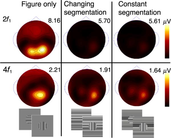
Figure region response distribution at the second (top) and fourth harmonic (bottom) under three background contexts. Response maxima are indicated above each map, and maps for each row are on the same scale. Two stimulus frames for each condition are presented below.

Discussion

In our previous study (Appelbaum et al., 2006), we used temporal tagging and EEG source imaging to demonstrate separate, largely cue-invariant processing streams for the figure and background regions of simple texture-defined forms. Here we show that the dominant region interaction (1f₁ + 1f₂), unlike the region responses themselves, depends strongly on orientation cues within the regions. Region interaction was also dependent on the spatial proximity of the two regions and the presence of a uniform field in the image sequence. We found border-related activity in both first-tier retinotopic areas and in a nonretinotopic region of extra-striate cortex that is displaced dorsally and anteriorally from the locus of maximal figure-region activity. The overall pattern of results suggests that although the mechanisms responsible for generating the region-interaction signals are sensitive to image discontinuities, they do not appear to be directly responsible for routing activity through the separate region response networks observed in our previous study.

Stimulus dependence of nonlinear spatio-temporal interactions

The presence of responses at frequencies that are low-order multiples of the input frequencies indicates that the two inputs have passed through a common nonlinear site, such as the spiking threshold of a cortical neuron. In our paradigm and similar ones (Norcia et al., 1999; Victor & Conte, 2000; Zemon & Ratliff, 1982), these responses are indicative of lateral interactions that either occur within or between receptive fields spanning separated regions of visual space.

In our first analysis, we showed that the strength of nonlinear region-interaction depends on the cues that defined the figure/ground segmentation. Activity at the second-order sum frequency (6.6 Hz) was present only when the textures comprising the figure and background regions had orientation information (the orientation-defined and phase-defined forms), but not when orientation information was absent (temporally defined form). While the presence of orientation information is critical for the generation of this type of figure-ground interaction, this is not the case for the fourth-order sum frequency. This response component, while small, is reliably present for all cue types.

In our second analysis, we found that when the figure and background regions were always segmented (e.g., lacked collinear states) that region-interaction was reduced (orientation cue) or eliminated (phase cue). A similar effect was reported in radially organized targets where nonlinear interactions were quenched by as little as 10° of angular phase misalignment (Zemon & Ratliff, 1982) and for offset gratings where the introduction of a 90° spatial shift between strips of gratings was sufficient to quench nonlinear interaction terms (Norcia et al., 1999). Neither study examined fourth-order terms that we show to be less dependent on spatial alignment than the dominant second-order term. Finally, like previous studies (Norcia et al., 1999; Victor & Conte, 2000; Zemon & Ratliff, 1982), we find that even very small gaps between regions are sufficient to produce dramatic reductions in nonlinear spatio-temporal interactions at the second-order sum frequency, but not at the fourth-order sum frequency.

Two patterns of spatio-temporal interaction

Our experiments suggest that there are at least two different types of nonlinear figure ground interaction. One type, indexed by the second-order sum term, is very sensitive to continuity/discontinuity in the image and the other, indexed by the fourth-order sum term, is not. The presence of the fourth-order sum, by itself, indicates that the figure/ground interaction is more complex than simply squaring or multiplying of the inputs. The fact that it shows different functional specificity than the second-order terms suggests that a single nonlinearity is not involved. If a single, high-order nonlinearity was present, it would generate both low- and high-order interaction terms and these would have the same functional specificity (for a detailed example, see Hou et al., 2003). Fourth-order spatio-temporal interaction has been observed in two previous low channel-count studies (Hou et al., 2003; Victor & Conte, 2000). Both studies modeled the fourth-order interaction as arising within a cascade of two nonlinear stages. Our finding here of a fourth-order interaction in the apparent absence of a second-order interaction (temporally defined forms) is consistent with a two stage model where the nonoriented texture is first rectified within a region and is then pooled across regions at a second nonlinear stage.

The simplest model of the nonlinear region interaction components has the interaction occurring within receptive fields that span both regions. On this view, the interaction would cease once elements from the figure and background are too widely separated to fall within the relevant receptive fields. For this model to hold for our data, the relevant receptive fields would have to be extremely small on the order of 5-10 arcmin. Recent cortical surface recordings suggest that most receptive fields in human cortex are substantially larger than this (Yoshor, Bosking, Ghose, & Maunsell, 2007). Moreover, average receptive field size grows by a factor of more than four between calcarine cortex and lateral cortical areas that include TOPJ and MT+ (Yoshor et al., 2007). We would thus expect that if receptive field size per se were the critical factor limiting nonlinear interaction, that the gap function would be progressively broader in extra-striate areas. We did not observe this in any of the retinotopic areas, nor did we observe an expanded interaction range in nonretino-topic cortex at the temporal occipital parietal junction (TOPJ). The strong dependence of the interaction terms on collinear versus discontinuous texture may thus be more the result of more complex network properties than of simple feed-forward integration within classical receptive fields.

A recent study of lateral interactions in area 17 of the anesthetized cat (Biederlack et al., 2006) has also suggested that there are two distinct modes of interaction between regions of disk/annulus stimuli. That study found that single and multiunit responses to a drifting disk were maximally suppressed when the annulus had the same orientation as the central disk. However, when the disk and annulus were of the same orientation, there was no effect on firing rate of the relative spatial phase and thus the segmentation state of the disk and annulus. In this case, a change in the synchronization of responses to the center was observed, with greater synchronization occurring when the stimuli were segmented. Our results are at least partially consistent with their findings. We find that the changing orientation background has a similar suppressive effect on the figure-region responses that does not depend on the segmentation state when the figure and background share the same orientation (2f₁ and 4f₁ responses; Figure 8). However, the fact that the strength of nonlinear interaction (1f₁ + 1f₂, 2f₁ + 2f₂; Figures 4 and 5) depends on the relative phase of the regions indicates the presence of a rate code for stimulus phase. Intermodulation responses still carry the temporal signature of the two input frequencies and are thus a form of rate coding. Our measurements are not sensitive to synchrony effects that may also be present in our recordings. It will be of interest in the future to determine if similar mechanisms underlie synchrony and intermodulation effects. At this point, we can only say that both appear to depend on the presence of collinear texture, perhaps in a complementary fashion.

Functional specificity of the TOPJ

As shown in Figure 4 (row 3) the distribution of sum-term responses to the phase- and orientation-defined forms shows activity in both first-tier visual areas (V1-V3) and in regions of extra-striate cortex that extend between retinotopic areas V3A and hMT+. This activity occurs near the border of the temporal, occipital and parietal cortex and we thus referred to this region as the temporal occipital parietal junction (TOPJ) when doing ROI-based analysis. The mean Talairach coordinates for this ROI are similar to those of the kinetic occipital region (Dupont et al., 1997). This area was originally defined on the basis of motion-defined borders between strips of moving texture and thus the defining stimulus shares some similarity to our dynamic second-order forms. A more recent study (Tyler, Likova, Kontsevich, & Wade, 2006) has argued that this area responds more generally to depth structure. Depth ordering is apparent in our displays (the figure appears to be in front of the background) and this may be a common factor across our study and that of Tyler et al.

The role of border interactions in determining the fate of regions

Looking across each of our experimental manipulations, we find that although the sum term is strongly affected by what would generally be considered border discontinuity signals, this particular signal does not appear to control the process by which the figure region is routed to lateral cortex and the background to more dorsal areas as described in our previous analysis of region responses (Appelbaum et al., 2006). Even though the sum term is weak (or absent) for the temporally defined from and for the constantly segmented phase-defined form stimuli, these stimuli still segment perceptually and the figure and background regions are processed through the same complementary cortical networks that are activated by stimuli that do generate sum-term responses. Each cue type elicited a small, but measurable fourth-order sum term (2f₁ + 2f₂). It is possible that this border-related signal (see gap functions) is important in initiating region segmentation since it is always present. It is also possible that border signals we have measured at the interaction frequencies are not the critical determinants of segmentation and routing through cortex of figure and background regions, but rather it could be that the temporal differences between regions are themselves sufficient. Previous models of segmentation (see Introduction) have generally suggested that discontinuities in orientation, color, motion direction, or disparity feature maps cues are key components in the segmentation process. However, these models have, with the exception of models of motion segmentation, dealt with static stimuli and have not considered temporal differences per se as cues to segmentation. Temporal coherence across regions is sufficient to support perceptual segmentation (Kandil & Fahle, 2003; Likova & Tyler, 2005; Rogers-Ramachandran & Ramachandran, 1998) and, with stimuli such as ours, is sufficient to lead to separate region-processing networks.

Conclusions

In this paper, we use multi-input nonlinear analysis methods and EEG source imaging to characterize nonlinear spatial interactions occurring between figure and background regions of texture defined stimuli. We show that nonlinear responses are present in both retinotopic and extra-striate visual areas and that the amount of nonlinear interaction depends strongly on the type of feature defining the segmentation. Figure/background interaction was greatly diminished by the elimination of orientation cues, the introduction of small gaps between the two regions, or by the presence of a constant second-order border between regions. These results suggest that temporal coherence across regions is sufficient to support the spatial segmentation of a stimulus and to activate region-processing neuronal networks.

References

- Allman J, Miezin F, McGuinness E. Direction- and velocity-specific responses from beyond the classical receptive field in the middle temporal visual area (MT) Perception. 1985;14:105–126. doi: 10.1068/p140105. [DOI] [PubMed] [Google Scholar]
- Angelucci A, Bressloff PC. Contribution of feedforward, lateral and feedback connections to the classical receptive field center and extra-classical receptive field surround of primate V1 neurons. Progress in Brain Research. 2006;154:93–120. doi: 10.1016/S0079-6123(06)54005-1. [DOI] [PubMed] [Google Scholar]
- Appelbaum LG, Wade AR, Vildavski VY, Pettet MW, Norcia AM. Cue-invariant networks for figure and background processing in human visual cortex. Journal of Neuroscience. 2006;26:11695–11708. doi: 10.1523/JNEUROSCI.2741-06.2006. [DOI] [PMC free article] [PubMed] [Google Scholar]
- Bach M, Meigen T. Electrophysiological correlates of texture segregation in the human visual evoked potential. Vision Research. 1992;32:417–424. doi: 10.1016/0042-6989(92)90233-9. [DOI] [PubMed] [Google Scholar]
- Baitch LW, Levi DM. Evidence for nonlinear binocular interactions in human visual cortex. Vision Research. 1988;28:1139–1143. doi: 10.1016/0042-6989(88)90140-x. [DOI] [PubMed] [Google Scholar]
- Biederlack J, Castelo-Branco M, Neuenschwander S, Wheeler DW, Singer W, Nikolić D. Brightness induction: Rate enhancement and neuronal synchronization as complementary codes. Neuron. 2006;52:1073–1083. doi: 10.1016/j.neuron.2006.11.012. [DOI] [PubMed] [Google Scholar]
- Blakemore C, Tobin EA. Lateral inhibition between orientation detectors in the cat's visual cortex. Experimental Brain Research. 1972;15:439–440. doi: 10.1007/BF00234129. [DOI] [PubMed] [Google Scholar]
- Brewer AA, Liu J, Wade AR, Wandell BA. Visual field maps and stimulus selectivity in human ventral occipital cortex. Nature Neuroscience. 2005;8:1102–1109. doi: 10.1038/nn1507. [DOI] [PubMed] [Google Scholar]
- Burton GJ. Evidence for non-linear response processes in the human visual system from measurements on the thresholds of spatial beat frequencies. Vision Research. 1973;13:1211–1225. doi: 10.1016/0042-6989(73)90198-3. [DOI] [PubMed] [Google Scholar]
- Candy TR, Skoczenski AM, Norcia AM. Normalization models applied to orientation masking in the human infant. Journal of Neuroscience. 2001;21:4530–4541. doi: 10.1523/JNEUROSCI.21-12-04530.2001. [DOI] [PMC free article] [PubMed] [Google Scholar]
- DeYoe EA, Carman GJ, Bandettini P, Glickman S, Wieser J, Cox R, et al. Mapping striate and extrastriate visual areas in human cerebral cortex. Proceedings of the National Academy of Sciences of the United States of America. 1996;93:2382–2386. doi: 10.1073/pnas.93.6.2382. [DOI] [PMC free article] [PubMed] [Google Scholar]
- Dupont P, De Bruyn B, Vandenberghe R, Rosier AM, Michiels J, Marchal G, et al. The kinetic occipital region in human visual cortex. Cerebral Cortex. 1997;7:283–292. doi: 10.1093/cercor/7.3.283. [DOI] [PubMed] [Google Scholar]
- Grill-Spector K, Kushnir T, Edelman S, Itzchak Y, Malach R. Cue-invariant activation in object-related areas of the human occipital lobe. Neuron. 1998;21:191–202. doi: 10.1016/s0896-6273(00)80526-7. [DOI] [PubMed] [Google Scholar]
- Grossberg S, Mingolla E. Neural dynamics of perceptual grouping: Textures, boundaries, and emergent segmentations. Perception & Psychophysics. 1985;38:141–171. doi: 10.3758/bf03198851. [DOI] [PubMed] [Google Scholar]
- Hou C, Pettet MW, Sampath V, Candy TR, Norcia AM. Development of the spatial organization and dynamics of lateral interactions in the human visual system. Journal of Neuroscience. 2003;23:8630–8640. doi: 10.1523/JNEUROSCI.23-25-08630.2003. [DOI] [PMC free article] [PubMed] [Google Scholar]
- Huk AC, Dougherty RF, Heeger DJ. Retinotopy and functional subdivision of human areas MT and MST. Journal of Neuroscience. 2002;22:7195–7205. doi: 10.1523/JNEUROSCI.22-16-07195.2002. [DOI] [PMC free article] [PubMed] [Google Scholar]
- Johnson RA, Wichern DW. Applied multivariate statistical analysis. Prentice Hall; Upper Saddle River, NJ: 1998. pp. 236–239. [Google Scholar]
- Kandil FI, Fahle M. Electrophysiological correlates of purely temporal figure-ground segregation. Vision Research. 2003;43:2583–2589. doi: 10.1016/s0042-6989(03)00456-5. [DOI] [PubMed] [Google Scholar]
- Keselman HJ, Algina J, Kowalchuk RK. The analysis of repeated measures designs: A review. British Journal of Mathematical and Statistical Psychology. 2001;54:1–20. doi: 10.1348/000711001159357. [DOI] [PubMed] [Google Scholar]
- Koechlin E, Anton JL, Burnod Y. Bayesian inference in populations of cortical neurons: A model of motion integration and segmentation in area MT. Biological Cybernetics. 1999;80:25–44. doi: 10.1007/s004220050502. [DOI] [PubMed] [Google Scholar]
- Kourtzi Z, Kanwisher N. Cortical regions involved in perceiving object shape. Journal of Neuroscience. 2000;20:3310–3318. doi: 10.1523/JNEUROSCI.20-09-03310.2000. [DOI] [PMC free article] [PubMed] [Google Scholar]
- Lamme VA, Van Dijk BW, Spekreijse H. Texture segregation is processed by primary visual cortex in man and monkey. Evidence from VEP experiments. Vision Research. 1992;32:797–807. doi: 10.1016/0042-6989(92)90022-b. [DOI] [PubMed] [Google Scholar]
- Landy MS, Bergen JR. Texture segregation and orientation gradient. Vision Research. 1991;31:679–691. doi: 10.1016/0042-6989(91)90009-t. [DOI] [PubMed] [Google Scholar]
- Li Z. Pre-attentive segmentation in the primary visual cortex. Spatial Vision. 2000;13:25–50. doi: 10.1163/156856800741009. [DOI] [PubMed] [Google Scholar]
- Likova LT, Tyler CW. Transient-based image segmentation: Top-down surround suppression in human V1. SPIE Proceedings Series. 2005;5666:248–257. [Google Scholar]
- Lin FH, Witzel T, Ahlfors SP, Stufflebeam SM, Belliveau JW, Haämaälaäinen MS. Assessing and improving the spatial accuracy in MEG source localization by depth-weighted minimum-norm estimates. Neuroimage. 2006;31:160–171. doi: 10.1016/j.neuroimage.2005.11.054. [DOI] [PubMed] [Google Scholar]
- Malach R, Reppas JB, Benson RR, Kwong KK, Jiang H, Kennedy WA, et al. Objectrelated activity revealed by functional magnetic resonance imaging in human occipital cortex. Proceedings of the National Academy of Sciences of the United States of America. 1995;92:8135–8139. doi: 10.1073/pnas.92.18.8135. [DOI] [PMC free article] [PubMed] [Google Scholar]
- Malik J, Perona P. Preattentive texture discrimination with early vision mechanisms. Journal of the Optical Society of America A, Optics and Image Science. 1990;7:923–932. doi: 10.1364/josaa.7.000923. [DOI] [PubMed] [Google Scholar]
- Marcar VL, Loenneker T, Straessle A, Jaggy S, Kucian K, Martin E. An fMRI study of the cerebral macro network involved in `cue invariant' form perception and how it is influenced by stimulus complexity. Neuroimage. 2004;23:947–955. doi: 10.1016/j.neuroimage.2004.05.028. [DOI] [PubMed] [Google Scholar]
- Marcus DS, Van Essen DC. Scene segmentation and attention in primate cortical areas V1 and V2. Journal of Neurophysiology. 2002;88:2648–2658. doi: 10.1152/jn.00916.2001. [DOI] [PubMed] [Google Scholar]
- Nelson JI, Frost BJ. Orientation-selective inhibition from beyond the classic visual receptive field. Brain Research. 1978;139:359–365. doi: 10.1016/0006-8993(78)90937-x. [DOI] [PubMed] [Google Scholar]
- Norcia AM, Wesemann W, Manny RE. Electrophysiological correlates of vernier and relative motion mechanisms in human visual cortex. Visual Neuroscience. 1999;16:1123–1131. doi: 10.1017/s0952523899166124. [DOI] [PubMed] [Google Scholar]
- Nothdurft HC. Texture segmentation and popout from orientation contrast. Vision Research. 1991;31:1073–1078. doi: 10.1016/0042-6989(91)90211-m. [DOI] [PubMed] [Google Scholar]
- Regan D. Human brain electrophysiology: Evoked potentials and evoked magnetic fields in science and medicine. Elsevier; New York: 1989. [Google Scholar]
- Regan D, Regan MP. Nonlinearity in human visual responses to two-dimensional patterns, and a limitation of Fourier methods. Vision Research. 1987;27:2181–2183. doi: 10.1016/0042-6989(87)90132-5. [DOI] [PubMed] [Google Scholar]
- Roelfsema PR, Lamme VA, Spekreijse H, Bosch H. Figure-ground segregation in a recurrent network architecture. Journal of Cognitive Neuroscience. 2002;14:525–537. doi: 10.1162/08989290260045756. [DOI] [PubMed] [Google Scholar]
- Rogers-Ramachandran DC, Ramachandran VS. Psychophysical evidence for boundary and surface systems in human vision. Vision Research. 1998;38:71–77. doi: 10.1016/s0042-6989(97)00131-4. [DOI] [PubMed] [Google Scholar]
- Song Y, Baker CL. Neural mechanisms mediating responses to abutting gratings: Luminance edges vs. illusory contours. Visual Neuroscience. 2006;23:181–199. doi: 10.1017/S0952523806232036. [DOI] [PubMed] [Google Scholar]
- Sutter A, Graham N. Investigating simple and complex mechanisms in texture segregation using the speed-accuracy tradeoff method. Vision Research. 1995;35:2825–2843. doi: 10.1016/0042-6989(95)00045-2. [DOI] [PubMed] [Google Scholar]
- Thielscher A, Neumann H. Neural mechanisms of cortico-cortical interaction in texture boundary detection: A modeling approach. Neuroscience. 2003;122:921–939. doi: 10.1016/j.neuroscience.2003.08.050. [DOI] [PubMed] [Google Scholar]
- Tootell RB, Hadjikhani N. Where is `dorsal V4' in human visual cortex? Retinotopic, topographic and functional evidence. Cerebral Cortex. 2001;11:298–311. doi: 10.1093/cercor/11.4.298. [DOI] [PubMed] [Google Scholar]
- Tyler CW, Likova LT, Kontsevich LL, Wade AR. The specificity of cortical region KO to depth structure. Neuroimage. 2006;30:228–238. doi: 10.1016/j.neuroimage.2005.09.067. [DOI] [PubMed] [Google Scholar]
- Valdes-Sosa P, Marti F, Garcia F, Casanova R. Variable resolution electric-magnetic tomography. Biomagnetism 96: Proceedings of the 10th International Conference Biomagnetism.1996. pp. 373–376. [Google Scholar]
- Victor J, Shapley R. A method of nonlinear analysis in the frequency domain. Biophysical Journal. 1980;29:459–483. doi: 10.1016/S0006-3495(80)85146-0. [DOI] [PMC free article] [PubMed] [Google Scholar]
- Victor JD, Conte MM. Two-frequency analysis of interactions elicited by Vernier stimuli. Visual Neuroscience. 2000;17:959–973. doi: 10.1017/s0952523800176151. [DOI] [PubMed] [Google Scholar]
- Victor JD, Mast J. A new statistic for steady-state evoked potentials. Electroencephalography and Clinical Neurophysiology. 1991;78:378–388. doi: 10.1016/0013-4694(91)90099-p. [DOI] [PubMed] [Google Scholar]
- Vuilleumier P, Henson RN, Driver J, Dolan RJ. Multiple levels of visual object constancy revealed by event-related fMRI of repetition priming. Nature Neuroscience. 2002;5:491–499. doi: 10.1038/nn839. [DOI] [PubMed] [Google Scholar]
- Wade AR, Brewer AA, Rieger JW, Wandell BA. Functional measurements of human ventral occipital cortex: Retinotopy and colour. Philosophical Transactions of the Royal Society of London B: Biological Sciences. 2002;357:963–973. doi: 10.1098/rstb.2002.1108. [DOI] [PMC free article] [PubMed] [Google Scholar]
- Yoshor D, Bosking WH, Ghose GM, Maunsell JH. Receptive fields in human visual cortex mapped with surface electrodes. Cerebral Cortex. 2007;17:2293–2302. doi: 10.1093/cercor/bhl138. [DOI] [PubMed] [Google Scholar]
- Zemon V, Ratliff F. Visual evoked potentials: Evidence for lateral interactions. Proceedings of the National Academy of Sciences of the United States of America. 1982;79:5723–5726. doi: 10.1073/pnas.79.18.5723. [DOI] [PMC free article] [PubMed] [Google Scholar]
- Zemon V, Ratliff F. Intermodulation components of the visual evoked potential: Responses to lateral and superimposed stimuli. Biological Cybernetics. 1984;50:401–408. doi: 10.1007/BF00335197. [DOI] [PubMed] [Google Scholar]
Associated Data
This section collects any data citations, data availability statements, or supplementary materials included in this article.