COMBE: Complex-Model-Based Estimation of Thermal Noise for fMRI Data in the Presence of Artifacts

Abstract

Due to the presence of artifacts induced by fast-imaging acquisition in functional MRI studies, it is very difficult to estimate the variance of thermal noise by traditional methods in magnitude images. Moreover, the existence of incidental phase fluctuations impair the validity of currently available solutions based on complex datasets. In this paper, a time-domain model is proposed to generalize the analysis of complex datasets for nonbrain regions by incorporating artifacts and phase fluctuations. Based on this model, a novel estimation schema has been developed to find an appropriate set of voxels in the nonbrain region according to their levels of artifact and phase fluctuation. In addition, the noise intensity from these voxels is estimated. The whole schema is named the Complex-Model-Based Estimation (COMBE). Theoretical and experimental results demonstrate that the proposed COMBE method provides a better estimation of thermal noise in fMRI studies than previously proposed methods, and suggest that the new method can adapt to a broader range of applications, such as functional connectivity studies, evaluation of sequence designs and reconstruction schemas.

INTRODUCTION

Thermal noise in MR images is a very important parameter. The estimation of thermal noise not only provides the measurement of quality of an MRI system [1], and quantification of an MR signal, especially signal-to-noise ratio (SNR) for functional MRI (fMRI) signal [2], but also offers a general measure to evaluate the performance of MRI sequences [3] and reconstruction schemas [4].

The analytical estimation methods that determine the thermal noise have been extensively studied. In most cases, the thermal noise is determined from magnitude images, which can be modeled as a Rician distribution that has no analytical solution. When the signal-to-noise ratio (SNR) is high, the Rician distribution can be approximated as Gaussian in nature and thermal noise can be estimated as the standard deviation of the magnitude [5]. When the signal is zero the Rician model evolves to a Rayleigh distribution and thermal noise can be estimated by dividing the standard deviation of the magnitude with a correctional factor (about 0.655) [6,7].

Technological development and clinical research applications of functional MRI (fMRI) methods have generated three new challenges in estimating noise. First, unlike anatomical images, fMRI datasets in high SNR regions such as the brain contain significant temporal signal changes, hence, invalidating the Gaussian method. The temporal signal changes may include the fluctuations in blood oxygenation level-dependent (BOLD) signals induced by tasks or physiologic noise during rest [8]. Second, the presence of significant artifacts in the background regions (nonbrain regions), acquired by fast imaging methods, such as EPI [9] and spiral [10] pulse sequences, make the Rayleigh method inapplicable. To solve this problem, researchers have developed several methods, including averaging variances over real and imaginary channels (Average method) [11-13], maximum likelihood (ML)-based estimations [12,14], and the double-acquisition method employing the analytical form of even moments of the Rician distribution [15].

The final problem seen in fMRI datasets is the incidental phase fluctuations, which are derived from various time-dependent sources of variation, including flip angle inhomogeneity, filter responses, system delay, noncentered sampling windows, etc. [16]. However, the abovementioned methods did not explicitly take the phase fluctuation into account as a random variable.

In this paper, a new method is proposed for fMRI datasets. It estimates the thermal noise in the presence of image artifacts and phase fluctuations for fMRI datasets. By analyzing real and imaginary channels of complex-valued data in the time domain, it becomes evident that thermal noise can be accurately estimated. Theoretical simulations and experimental results demonstrate that the new method provides better estimation of thermal noise and a higher capacity for a broader range of artifact-to-noise ratios (ANRs) and phase fluctuations than the previously proposed methods. Thus, the new method is suitable for various applications, including functional connectivity studies, sequence and reconstruction evaluations.

THEORY

It is well known that within the brain, the real R_b(t)and imaginary I_b(t) channels in a given voxel of reconstructed fMRI datasets have three components. These components are: the magnitude of the signal S(t), the phase of the signal θ(t), and thermal noise n(t) at time t. The time-domain model within a given voxel can be expressed as:

$$\begin{array}{cc}{R}_b\left(t\right)& =S\left(t\right)\cos \left(\theta \left(t\right)\right)+n_1\left(t\right)\\ I_b\left(t\right)& =S\left(t\right)\sin \left(\theta \left(t\right)\right)+n_2\left(t\right)\end{array}$$ (1)

where n₁(t) and n₂(t) are additive thermal measurement noise [17,18]. As previously described, the magnitude and phase portions of the signal are temporally varying quantities. Thus, they may be modeled by temporally constant mean- and time-varying portions S(t) = S + ΔS(t) and θ(t) = θ + Δθ(t). The temporally constant means of the magnitude and phase are S and θ, while their time-varying portions are ΔS(t) and Δθ(t) respectively.

Any signal that is present in the background region of the reconstructed fMRI datasets is due to ghosting artifacts. Thus, it is described by a decreased version of the original signal. The original magnitude signal S(t) in Eq. (1) is decreased by an artifact proportionality factor γ to yield γS(t) = γS + γΔS(t) instead of S(t) for an artifact-to-noise model.

In fMRI data, the mean magnitude signal is usually much larger than its temporal variation, S ≫ ΔS(t), so that the artifact magnitude signal is also much larger than its temporal variation, γS ≫ γΔS(t). This allows the variation of the artifact signal to be neglected when γS(t) is comparable to the thermal noise. Thus, the artifact γS(t) can be taken as a temporally constant quantity a, called the artifact level. The artifact-to-noise complex model can be written as:

$$\begin{array}{cc}R\left(t\right)& =a\cos \left(\theta +\Delta \theta \left(t\right)\right)+n_1\left(t\right)\\ I\left(t\right)& =a\sin \left(\theta +\Delta \theta \left(t\right)\right)+n_2\left(t\right).\end{array}$$ (2)

In non-artifact voxels a = 0, so that the real and imaginary channels consist only of noise. The phase fluctuation Δθ(t) in fMRI data is relatively small. This allows Eq. (2) to be written as:

$$\begin{array}{cc}R\left(t\right)=a\cos \left(\theta \left(t\right)\right)+n_1\left(t\right)& \approx a\left(\cos \theta -\sin \theta ·\mathrm{\Delta }\theta \left(t\right)\right)+n_1\left(t\right)\\ I\left(t\right)=a\sin \left(\theta \left(t\right)\right)+n_2\left(t\right)& \approx a\left(\sin \theta +\cos \theta ·\mathrm{\Delta }\theta \left(t\right)\right)+n_2\left(t\right)\end{array}$$ (3)

with the use of the Trigonometric addition formulas for Sines and Cosines along with small angle approximations.

By definition, the thermal noise n₁(t) and n₂(t) in the two channels are mutually independent and identically distributed with means that are zero and variances σ₀². Additionally, the mean and variance of the phase fluctuation are zero and σ_θ². With the above model specifications, the mean (expected) value for the real and imaginary parts of the artifact-to-noise complex model are:

$$\begin{array}{cc}{\mu }_R& =a\cos \theta \\ {\mu }_I& =a\sin \theta \end{array}$$ (4)

while their variances are:

$$\begin{array}{cc}{\sigma }_R^2& =a^2{\sin }^2\theta ·{\sigma }_{\theta }^2+{\sigma }_0^2\\ {\sigma }_I^2& =a^2{\cos }^2\theta ·{\sigma }_{\theta }^2+{\sigma }_0^2.\end{array}$$ (5)

Since we do not assume any particular distribution for the thermal noise and phase fluctuations, we do not have a likelihood, and cannot estimate the model parameters with maximum likelihood estimates (MLEs). Instead, we will estimate the model parameters with method of moment estimators (MMEs). MMEs are found by equating the population moments to the sample moments [19]. The MMEs for the artifact level a and mean phase θ are found by equating the population means to the sample means (first moments). This yields the equations:

$$\overline{R}=\widehat{a}\cos \left(\widehat{\theta }\right)\overline{I}=\widehat{a}\sin \left(\widehat{\theta }\right)$$ (6)

where R̄ and Ī are the sample means of the real and imaginary channels. The solution to these two equations with two unknowns yields MMEs that are:

$$\widehat{a}=\sqrt{{\left(\overline{R}\right)}^2+{\left(\overline{I}\right)}^2}\widehat{\theta }={\tan }^{-1}\left(\overline{I}/\overline{R}\right)$$ (7)

For convenience, â is named the artifact level, while θ̂ is called estimated phase mean. The MMEs for the variances σ₀² and σ_θ² can be found by equating the population second moments to the sample second moments. This yields the equations:

$$\begin{array}{cc}{\widehat{\sigma }}_R^2=\overline{R^2}-{\left(\overline{R}\right)}^2& ={\widehat{a}}^2{\sin }^2\widehat{\theta }·{\widehat{\sigma }}_{\theta }^2+{\widehat{\sigma }}_0^2\\ {\widehat{\sigma }}_I^2=\overline{I^2}-{\left(\overline{I}\right)}^2& ={\widehat{a}}^2{\cos }^2\widehat{\theta }·{\widehat{\sigma }}_{\theta }^2+{\widehat{\sigma }}_0^2\end{array}$$ (8)

where $\overline{R^2}$ and $\overline{I^2}$ are the means of the squares of the real and imaginary channels respectively while R̄ and Ī remain as previously defined. The solution to these two equations with the two unknowns yields the following MMEs:

$$\begin{array}{ll}{\widehat{\sigma }}_{\theta }^2& =\frac{{\widehat{\sigma }}_I^2-{\widehat{\sigma }}_R^2}{{\widehat{a}}^2\cos \left(2\widehat{\theta }\right)}\\ {\widehat{\sigma }}_0^2& =\frac{1}{2}\left({\widehat{\sigma }}_R^2+{\widehat{\sigma }}_I^2\right)-\frac{1}{2}{\widehat{a}}^2{\widehat{\sigma }}_{\theta }^2\end{array}$$ (9)

It is noted that in Eq. (9), the denominator for the estimate of the sample variance for the phase fluctuation will approach zero when the estimated phase mean θ̂ is close to (π/4)·(2k −1) where K is any integer. To avoid this problem, a complementary set of equations is introduced:

$$\begin{array}{cc}{\widehat{\sigma }}_{R+I}^2=\overline{{(R+I)}^2}-{\left(\overline{R+I}\right)}^2& ={\widehat{a}}^2{\widehat{\sigma }}_{\theta }^2\left(1-\sin \left(2\widehat{\theta }\right)\right)+2{\widehat{\sigma }}_0^2\\ {\widehat{\sigma }}_{R-I}^2=\overline{{(R-I)}^2}-{\left(\overline{R-I}\right)}^2& ={\widehat{a}}^2{\widehat{\sigma }}_{\theta }^2\left(1+\sin \left(2\widehat{\theta }\right)\right)+2{\widehat{\sigma }}_0^2\end{array}$$ (10)

The terms ${\widehat{\sigma }}_{R+I}^2$ and ${\widehat{\sigma }}_{R-I}^2$ represent the estimated variance of the sum of and the difference between the channels, respectively. Then, the sample variance for the phase fluctuation can be obtained as below:

$${\widehat{\sigma }}_{\theta }^2=\frac{{\widehat{\sigma }}_{R-I}^2-{\widehat{\sigma }}_{R+I}^2}{2{\widehat{a}}^2\sin 2\widehat{\theta }}$$ (11)

For convenience, this model will be parameterized by an artifact-to-noise ratio (ANR) that is defined as η = â/σ̂₀. This proposed method is named Complex Model-Based Estimation (COMBE).

For evaluation, the four previously proposed noise-estimation methods (Gaussian, Rayleigh, Average, and Simplex), are implemented for comparison through theoretical simulation and experimental determination of the estimated noise level. In the case of the Gaussian method, the artifact level can be estimated in the usual way as the sample mean of the magnitude time course, â_G = M̄ where $M\left(t\right)=\sqrt{{\left(R\left(t\right)\right)}^2+{\left(I\left(t\right)\right)}^2}$ denotes the magnitude at time t. The noise level can also be estimated from the voxel magnitude time courses as:

$${\widehat{\sigma }}_{0G}^2=\frac{1}{n-1}\sum _{t=1}^n{\left(M\left(t\right)-\overline{M}\right)}^2.$$ (12)

In this study, we implement this method, which is from the background region, in order to obtain a reference demonstrating how the ANR affects the estimation.

For the Rayleigh method, the artifact level can be estimated by ${\widehat{a}}_R=\sqrt{\frac{2}{\pi }{\widehat{\sigma }}_{0G}^2}$. The noise estimation is conducted by dividing the noise variance obtained from the Gaussian method with a constant factor as:

$${\widehat{\sigma }}_{0R}^2=\frac{{\widehat{\sigma }}_{0G}^2}{2-\pi /2}$$ (13)

as has been described previously [7]. The standard deviation of the noise is generally utilized. The widely used Rayleigh method selects the voxels from background regions and assumes these voxels contain only thermal noise without signal such as artifacts [17,20].

In the case of the Average method, the estimate of the artifact â_A is the same as our COMBE estimate. The estimate of the noise variance is the average of the variances of the real and imaginary datasets:

$${\widehat{\sigma }}_{0A}^2=\frac{1}{2}\left({\widehat{\sigma }}_R^2+{\widehat{\sigma }}_I^2\right).$$ (14)

The Average method was utilized on voxel measurements in space [8] assuming a region of constant amplitude and phase. This method was also used through time [14] in a model developed for fMRI, which has a temporally varying magnitude signal with a linear form and a temporally constant phase. We use the Average method that was developed for fMRI with a specification of a temporally constant magnitude since we have repeated measurements. This yields the same estimates as the version used in space, but we do not assume spatial homogeneity.

Although the Average method takes into account the existence of the artifact, it could produce a biased estimation when phase fluctuations exist. Our model explicitly assumes, mirrors, and estimates a phase fluctuation while the previous models do not. It should be noted that our COMBE MMEs for the mean artifact and phase are the same as the MLEs from the Average method. Further, in comparing the noise variance estimates in Eq. (9) to that in Eq. (14), the actual noise estimate by our COMBE method is:

$${\sigma }_0^2={\widehat{\sigma }}_{0A}^2-a^2{\sigma }_{\theta }^2/2.$$ (15)

Our COMBE MME for the noise variance is the same as the MLE from the Average method when there is no phase fluctuation. This demonstrates that our model is more general in nature, and that when phase fluctuations do not exist, our COMBE method produces an identical estimate of the noise variance as the Average method. However, when phase fluctuations exist, the two methods deviate from our estimate. The noise variances become decreased, accounting for the additional phase variation that we have modeled and estimated.

The Simplex method has a noise level that can be estimated based on the magnitude image by maximizing a two-dimensional function following the description by Sijbers et al. [12] (Eq.[46] in the cited paper). Although the Rician function cannot be analytically solved, a numerical optimization can be implemented by using the Nelder-Mead Simplex method [21].

SIMULATIONS AND RESULTS

A simulated data study was conducted in order to examine the theoretical properties of our COMBE model in comparison to the other previously described models under known conditions. Real R(t) and imaginary I(t) voxel time courses were generated according to the COMBE model in Eq. (3). This similarity to the experimental data will be presented in the next section. From these simulations, we can examine the impact of the ANR level and phase fluctuation standard deviation on the estimation of noise intensity under known conditions.

In statistical analysis, desirable properties of parameter estimates are unbiased (correct on average) and have the smallest standard deviation (on average). The smallest standard deviations that are unbiased are generally determined using the expected value and Cramer-Rao lower bound for the variance of an estimator from a model resulting in likelihood. However, since we do not make any distributional assumptions, we evaluate these properties via the Monte-Carlo simulation.

For our simulation, we utilized MATLAB to generate voxel time courses that are the length of 100 in order to mimic the experimental data that will be presented in the next section. The voxels were generated in an array where each element has a different ANR and thermal noise standard deviation. The phase mean θ for each voxel was randomly chosen by using a uniformly distributed random function from 0 to 2π radian, while the thermal noise standard deviation σ₀ was generated with channel-independent white Gaussian (normally) distributed noise with a mean of zero and a variance of one. The ANR was varied from zero to 5 from left to right along the horizontal direction. The phase fluctuation was generated with a zero mean and standard deviation σ_θ that was varied from zero to π / 2 radians from bottom to top. The ANR and phase fluctuation were both varied in 101 equally spaced increments. This procedure was repeated for 100 arrays of voxel time courses. The parameters for each of the models were estimated within each of the arrays. Array surfaces for the sample mean and Mean Square Error (MSE) of the estimated standard deviation of thermal noise by each method were computed as a function of the ANR and σ_θ².

The joint dependence of the thermal noise standard deviation as a function of the ANR and phase fluctuation standard deviation are presented as matrix maps in Figures 1 with color bar in Figure 1f, while the matrix maps for MSEs are omitted here. The true noise standard deviation in the figure is the one corresponding to the green region. We can see in Figure 1a that the Gaussian methods drastically underestimate the noise standard deviation for a low ANR, regardless of the phase fluctuation standard deviation. In Figure 1b we can see that the Rayleigh method drastically overestimates the noise standard deviation for a large ANR, regardless of the phase fluctuation standard deviation. Moreover, the Simplex method underestimates the standard deviation of noise when the ANR is low, as shown in Figure 1c. Nevertheless, in Figures 1d and e, we can see that the Average and COMBE methods more accurately estimate the noise standard deviation for a low to moderate ANR and phase fluctuation combinations. Further, the COMBE method performs better over a larger combination of ANRs and phase fluctuations, as seen by its green region in the lower left part of Figure 1e than the Average method with the green region in the lower left part of Figure 1d.

Figure 1.

Simulated estimation matrix maps for the five methods. The horizontal row of each matrix map corresponds to the ANR level from 0 to 5, while the vertical column corresponds to standard deviation of the phase fluctuant from 0 to π / 2. The estimated normalized standard deviation of thermal noise is color coded on the matrix map, especially with green corresponding to theoretical value 1. Figure 1a outlines the Gaussian method. Figure 1b represents the Rayleigh. Figure 1c is for the Simplex. Figure 1d is for the Average. Figure 1e is for the COMBE. Figure 1f is the illustration of the color coding. The horizontal dash lines superposed on the matrix maps represent a special case: σ_θ = 0.2, while the ANR changes from 0 to 5; and the vertical dash lines superposed on the matrix maps represent another special case: ANR=1, while σ_θ changes from 0 to π / 2.

The dependence of the thermal noise standard deviation estimate σ̂₀ on the ANR for each of the five noise-estimation methods is of interest. The 14^th row above describes mean arrays for the estimated noise standard deviation σ̂₀ corresponding to a typical value phase fluctuation standard deviation of 0.2 radian with an ANR varying from zero to five, as plotted in Figure 2a, with the MSE depicted in Figure 2b. As shown in Figure 2a, when the ANR is close to zero, the Gaussian method (in blue) drastically underestimates the noise, as does the Simplex method in black (but to a lesser extent). The Rayleigh method (in green) correctly estimates the noise. While the estimated noise levels for the Average and COMBE methods (in yellow and red) are accurate and relatively unbiased. As the ANR increases, the Rayleigh (in green) overestimates the noise and becomes more biased, while the Gaussian method yields a more unbiased estimate. The Average and COMBE method yield relatively unbiased estimates for the ANRs until about 2 and 4 respectively. The COMBE method with a smaller bias for all ANRs is considered. As seen in Figure 2b, the COMBE method (in red) produced the lowest overall variability, i.e., lowest MSEs for all ANRs considered among the five methods.

Figure 2.

Specific cases of the simulated estimations of thermal noise. The solid blue lines correspond to the Gaussian method; green lines are for the Rayleigh; black lines represent the Simplex; yellow lines are for the Average. The red lines are for the COMBE. Figure 2a presents the estimations when σ_θ is fixed at 0.2, while the ANR is scanned from 0 to 5, corresponding to the horizontal lines superposed on the matrix maps in Figures 1a to e; Figure 2b shows the MSE of the corresponding estimations; Figure 2c presents the estimations when the ANR is fixed at 1, while the σ_θ is scanned from 0 to π / 2, corresponding to the vertical dash lines superposed on the matrix maps in Figures 1a to e. Figure 2d shows the MSE of the corresponding estimations.

Also of interest within the simulation is the dependence of the thermal-noise standard deviation estimate on standard deviation of the phase fluctuation for each of the five noise-estimation methods. The 21^st row above describes mean array surfaces for the estimated noise standard deviation σ̂₀ corresponding to an ANR=1 with phase fluctuation standard deviation varying from zero to π / 2 radians, as plotted in Figure 2c. The MSEs of the estimation are plotted in Figure 2d, respectively. As shown in Figure 2c, since the ANR is fixed at one, the Gaussian and Simplex methods (in blue and black) remarkably underestimate the thermal noise, while the Rayleigh method (in green) significantly overestimates the noise. When the standard deviation of the phase fluctuation is small, both the Average and COMBE methods (in yellow and red) yield accurate and unbiased estimates. As the standard deviation of phase fluctuation increases, the Average method produces bias significantly more than the COMBE method. Overall, the latter consistently gives most accurate unbiased estimation of the noise standard deviation when σ_θ varied from 0 to π / 2 with an ANR=1. Figure 2d shows that the COMBE method (in red) consistently produces the lowest overall variability in terms of the MSE for the estimation of noise standard deviation among the five methods.

EXPERIMENTS AND RESULTS

All experimental fMRI data were obtained from a GE Signa 3.0 Tesla scanner (GE Medical Systems, Milwaukee, WI) using a single-channel receiving coil. The experiment was conducted on two healthy young subjects with approved protocol from the Institutional Review Board (IRB) and signed consent forms from the subjects. To demonstrate the performance of the five methods of noise estimation, a single shot, gradient echo continued fMRI EPI sequence was employed with the imaging parameters: TR of 1 s, TE of 30 ms, FOV of 24 cm, single slice covering with slice thickness of 4 mm, matrix size of 64 × 64, bandwidth of 125 KHz. There were 220 repetitions. Each fMRI scan was conducted using a continued EPI sequence with one axial slice across the upper part of the brain.

This continued EPI sequence is comprised of two parts. The first half scan used a 90-degree flip angle RF pulse, i.e., 110 repetitions of RF-ON scan. In the second half, the RF pulse was nullified, i.e., 110 repetitions in a RF-OFF scan. Therefore, the second half of the fMRI scan provided acquisition of pure thermal noise [4]. The RF-ON time courses that were extracted from the first half (discarding the first and last five time points) were utilized to examine and compare the performances of the five estimation methods. The RF-OFF time courses that were extracted from the second half (discarding the first and last five time points) were employed to estimate the underlying noise standard deviation. The estimated standard deviation of thermal noise for each method was defined as the average of the estimated standard deviations from all the RF-OFF time courses in the image, which were obtained by the corresponding method. Since there were no artifacts existing in the RF-OFF time courses, the estimation by the Average method was designated as the benchmark values. Figure 3 illustrates the data assignment for the processing from the continued EPI sequence. All five of the methods were applied to the RF-OFF time courses to compare their performances, and all the estimation results were normalized by the corresponding benchmark value and presented in Table 1. For Subject 1, the Gaussian method yielded the normalized RF-OFF estimate of the thermal noise standard deviation for the whole image as 0.6679, 1.0195 for the Rayleigh method, 1.00001 for the COMBE method, while it was 0.5451 for the Simplex method. For Subject 2, the RF-OFF estimates for the thermal noise standard deviation gave 0.6859 for the Gaussian, 1.0470 for the Rayleigh, 1.0003 for the COMBE, and 0.5601 for the Simplex. The COMBE method agrees with the Average method in estimating benchmark values.

Figure 3.

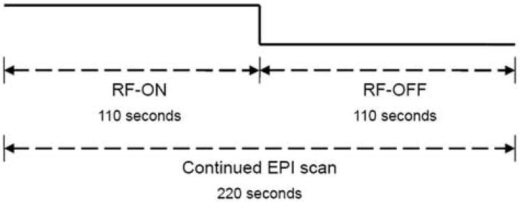
Illustration of the continued EPI data acquisition and corresponding RF-ON and RF-OFF datasets.

Table 1.

The estimation of thermal noise (normalized on the benchmark value) on RF-OFF time courses

	Gaussian	Rayleigh	Simplex	Average	COMBE
Subject 1	0.6679	1.0195	0.5451	1	1.0000
Subject 2	0.6859	1.0470	0.5601	1	1.0003

To further evaluate the five estimation methods, the following steps were taken with the RF-ON time courses. First, we segmented the brain region from the nonbrain region (background region) by using the plug-in “draw dataset” in the software package AFNI (Analysis of Functional NeuroImages) [22]. Then, each of the five methods was applied to every background voxel time course to obtain the voxelwise estimate of the artifact level, the standard deviation of phase fluctuation and the standard deviation of the thermal noise. With the benchmark value, i.e., the underlying standard deviation of thermal noise, the ANR for each voxel time course was available. Then, all the voxel time courses with a standard deviation of phase fluctuation less than 0.2 (determined by using Eq.(9)) and an ANR level no more than 10 were pooled together as the reliable voxel time course sets. For Subject 1, the number of background voxels (nonbrain region) was 2154, i.e., 52.59% of the whole-image voxels, while the number of reliable voxels reached 735, i.e., 17.94% of the whole-image voxels or 34.12% of the background voxels; for Subject 2, the number of background voxels (nonbrain region) was 2318, i.e., 56.59% of the whole-image voxels, while the number of reliable voxels reached 539, i.e., 13.15% of the whole-image voxels or 25.03% of the background voxels.

For each subject, within the reliable voxels, the estimated noise from each method was aggregated into ANR sets according to their corresponding ANRs. The aggregation of the estimation was based on rounding the ANRs to their nearest integers, e.g., a voxel time course with the ANR=3.7 was aggregated to the ANR=4 set, while the ANR=0.4 was included into the ANR=0 set. Within each ANR set, the mean value and MSE of the estimations were obtained. All the mean values of each ANR set were divided by the benchmark values to obtain the normalized estimation results. Thus, the dependency estimations of the ANR from the experiment data were at hand, which are also illustrated in Figure 4.

Figure 4.

Estimation of thermal noise on experimental results. The solid blue lines correspond to the Gaussian method; green lines are for the Rayleigh; black lines are for the Simplex; red lines are for the COMBE, while yellow lines are for the Average. Figure 2a presents the estimations for Subject 1, scanning the reliable background voxels with the ANR sets from 0 to 10. Figure 2b shows the MSEs of the corresponding estimations. Figure 2c presents the estimations for Subject 2; Figure 2b shows the MSEs of the corresponding estimations. The superposed gray horizontal bars in Figures 2a and c indicate the defined acceptable regions with ±10% of errors for the estimation of the standard deviation of the thermal noise.

The normalized estimation results are shown in the Figure 4 and listed in Table 2. As shown in the Figure 4, the five estimations repeat the pattern that was shown in Figure 2a: the Gaussian method underestimates when the ANR is small; the Rayleigh method overestimates over all the ANR levels; the Simplex method underestimates and introduces significant large variabilities, i.e., the MSEs; the Average method shows significant bias when the ANR increases; and the COMBE method yields much less bias through all the ANRs. Hence, it provides the most optimal estimation among the five methods. The normalized estimation results are also provided in Table 2. If we define ±10% as an acceptable range (superposed as gray bars on Figure 4a) for the estimation of the standard deviation of the thermal noise, then as seen in Figure 4a for Subject 1, the Gaussian method (in blue) is good from the ANR=2 to the ANR=10. The Rayleigh method (in green) has no good range. The Simplex method (in black) is reasonable from the ANR=7 to the ANR=10. The Average method (in yellow) is acceptable from the ANR=0 to the ANR=8. Finally, the COMBE method (in red) is superior to the other methods through all the ANR sets (0~10). The scan for Subject 2 presented more significant artifacts, and therefore, decreased acceptable regions for the estimation of all five methods. Still, the COMBE method outperforms all the others. As seen in Figure 4c for Subject 2, the acceptable range, i.e. ±10% error (superposed as gray bars on Figure 4c), for the Gaussian method (in blue) is ANR=2~5, no good range for the Rayleigh method (in green), ANR=3~6 for the Simplex method (in black), ANR=0~3 for the Average method (in yellow), while the COMBE method (in red) is superior to the other methods with the longest range: ANR=0~5. The COMBE method also produces the lowest MSE among all five methods for both subjects, as shown in Figures 4c and d. The histograms for the number of the reliable voxels for the subjects in terms of the ANR levels are presented in Figure 5.

Table 2.

The estimation of thermal noise (normalized mean value) on the integer ANR sets from the reliable background voxel time courses.

A. Estimation for subject 1
ANR	Gaussian	Rayleigh	Simplex	Average	COMBE
0	0.7318	1.1171	0.6605	0.9139	0.9072
1	0.8763	1.3375	0.7519	0.9643	0.9458
2	0.9622	1.4687	0.8215	1.0196	0.9849
3	0.9769	1.4911	0.7976	1.0224	0.9810
4	1.0019	1.5293	0.7854	1.0427	0.9965
5	1.0332	1.5771	0.9139	1.0716	1.0118
6	1.0109	1.5430	0.8815	1.0637	1.0057
7	1.0182	1.5542	0.9142	1.0853	1.0228
8	1.0273	1.5681	0.9061	1.0834	1.0262
9	1.0452	1.5954	0.9849	1.1457	1.0332
10	1.0290	1.5706	0.9088	1.1119	1.0231
B. Estimation for subject 2
ANR	Gaussian	Rayleigh	Simplex	Average	COMBE
0	0.7601	1.1602	0.6728	0.9522	0.9464
1	0.8870	1.3538	0.6941	0.9948	0.9765
2	0.9872	1.5069	0.8648	1.0421	1.0064
3	1.0387	1.5854	0.9048	1.0745	1.0235
4	1.0439	1.5934	0.9642	1.1031	1.0366
5	1.0923	1.6673	0.9615	1.1604	1.0833
6	1.1207	1.7107	1.0054	1.2458	1.1595
7	1.0440	1.5936	0.7610	1.1247	1.0546
8	1.1046	1.6860	0.8843	1.2145	1.1067
9	1.1757	1.7946	0.9680	1.3057	1.1834
10	1.1224	1.7133	0.9490	1.2670	1.1381

Figure 5.

Histogram of the reliable voxel sets regarding the ANR level. Figure 2a represents Subject 1; Figure 2b pertains to Subject 2. Vertical axis is the ration of number of voxels in each ANR set to the number of all the reliable voxels for each Subject.

DISCUSSION

For comparison, the five methods — Gaussian, Rayleigh, Simplex, Average, and COMBE — were employed to estimate the thermal noise in the fMRI datasets when a significant source of artifact noise was considered. With theoretical simulation and experimental fMRI datasets, the COMBE method, which we have described, provides the best noise estimation among the five. The Gaussian and Rayleigh methods cannot provide accurate and reliable estimates in the presence of artifacts. It is very difficult to select an artifact-free region in the magnitude images acquired by fast-imaging pulse sequences, such as EPI and spiral. Thus, a method that can tolerate the presence of artifacts is necessary. The Simplex method is very time consuming, easily trapped into local minimum, and cannot ensure accurate convergence for a considerable number of voxel time courses. The Average method can provide accurate thermal-noise estimation, if the phase fluctuations are small. However, our experimental results indicate that the phase fluctuations clearly exist, resulting in significant overestimation by the Average method. The newly proposed COMBE method not only employs the complex-valued dataset, thereby avoiding the disadvantages of the magnitude images, it can identify voxel sets based on the artifact levels and phase fluctuations with its step-by-step procedures.

It is important to clarify several key issues. First, the benchmark of the underlying standard deviation of the thermal noise is determined using the Average estimation from the RF-OFF time courses, which is extracted from the same continued EPI acquisition. In the past, thermal noise was determined by a separate scan with no RF pulse [4]. The continued scan further eliminates uncontrollable factors between the setups of the scans to ensure that the statistical characteristics of the thermal noise will not be changed. Although phantom studies have confirmed this assumption (data not shown here), the complexity involving human subjects can undermine the validation of the benchmark value by some unforeseeable causes. This issue needs further investigation.

There are several noticeable discrepancies between the theoretical simulation and experimental results. First, when the ANR increases, the COMBE method also begins to overestimate the thermal noise for the experiment data even with a restricted standard deviation of phase fluctuation (σ_θ < 0.2). This is primarily because the fluctuation of the artifacts in the time domain γΔS(t), which was described in the Theory Section, begins to play an observable role. None of the methods can avoid the effect of this fluctuation. The existence of significant artifact fluctuation in the large ANR situations is confirmed by the overestimation of the Gaussian method (in blue). This indicates that in addition to the thermal noise, there are other temporal magnitude fluctuations. It is interesting to note that even with the fluctuation of artifacts in play, the COMBE estimation performs at least as well as the Gaussian method. This demonstrates that both methods yield the combined variance of the thermal noise and artifact fluctuation, which are optimal under the circumstance. As stated in the Theory Section, the artifact proportionality γ determines what degree of artifact fluctuations will be ghosted into the background voxel time courses. The ghosted fluctuation γΔS(t) cannot be neglected when compared to the standard deviation of thermal noise σ₀. Therefore, the estimation will show some bias. In reality, those voxels with high ANR levels, which contain unneglectable artifact fluctuations can be excluded from the estimation to avoid contamination by the artifact fluctuation. Second, the Rayleigh method significantly overestimates the thermal noise even with the ANR=0 set, though theoretically it should give the correct answer. There are three possible causes. First, the ANR=0 set may include a significant portion of nonzero ANR voxel time courses, because the set is composed of voxel time courses with the ANR from 0 to 0.5. Or, the benchmark value possibly underestimates the thermal noise for the RF-ON time courses. The thermal noise may deviate slightly from the Gaussian distribution of real and imaginary channel data from the experimental data. Third, it is possible that the Simplex method significantly underperforms in the experimental data as compared to the simulations. We have come up with two explanations. Perhaps, the experimental data were more complicated, which imposed challenges on the Simplex method to reach the global minimum. Actually, there were a significant number of reliable voxel time courses that were rejected by the Matlab program due to divergence. The second premise is that the possible non-Gaussian nature of the thermal noise distribution, which undermines the foundation of the Simplex method is based on the Rician distribution of the voxel time courses.

Although the thermal noise has been viewed as independently Gaussian distributed in both I (real-part data) and Q (imaginary-part data) channels, this rule could be challenged. We investigated this in the experimental data by computing the kurtosis for the RF-OFF time courses. Theoretically, the kurtosis for a Gaussian-distributed random variable should be 3. In our data, they were 3.0818±0.5146 for I channel (real data), and 3.0701±0.5019 for Q channel (imaginary data) for Subject 1; 3.0718±0.5048 for I channel (real data), and 3.0628±0.4977 for Q channel (imaginary data) for Subject 2. Also, we conducted a simulation with matched datasets (4096 Gaussian distributed voxel time courses with 100 time points) in Matlab, the simulated kurtosis was 3.0008±0.4938. The difference is not statistically significant. However, the difference between the mean values, which usually will be taken as the ultimate estimation results, is noticeable. In addition, in the RF-OFF time courses, the Rayleigh method still overestimates the thermal noise by nearly 2% for Subject 1 and 5% for Subject 2. Though the discrepancy of the statistical characteristics can be neglected in most circumstances, it does diminish the validation of the Rayleigh method, as well as the Simplex method.

Even though the real-noise data show slight deviation from Gaussian distribution, we still recommend disregarding this issue in conventional linear reconstructed fMRI data. Still, recent emerging nonlinear reconstruction schema presented non-Gaussian distributed thermal noise [23-25], and rendered the magnitude image incapable of being modeled as Rician distribution [26]. This invalidated both the Rayleigh and Simplex methods. The COMBE method does not assume a specific statistical distribution for the thermal noise. Therefore, it can adapt to new reconstruction schemes that do not produce Gaussian noise, as long as they retain the independence of the I and Q channels, and remain stationary of the thermal noise in the time domain. The Average method in Eq.(14) does not have to rely on the premise of the Gaussian distribution of the thermal noise. However, the ML approaches cannot be used to reach the Average method.

There are two goals for noise estimation. First, the emphasis is overall noise estimation, which assumes that the same noise distribution in the whole image remains identical over both the spatial and time domains. Therefore, by collecting a sufficient number of voxels, the COMBE method can yield an optimal estimate. Parallel imaging such as SENSE [27] yields noise that is not uniform over the image. The proposed COMBE method can be implemented for individual voxel noise estimation. Because of its broad adaptive capability, it can be applied to more types of voxels with different properties than other methods listed in this study.

In current high field studies, the SNR is generally sufficient for most applications, which makes the noise estimation a less important topic in regular BOLD activation studies. However, there are still two fields which require accurate noise estimation. One is functional connectivity studies, which focus on one sort of physiologic noise — spontaneous low-frequency fluctuation. The intensity of the fluctuation is comparable to the standard deviation of the thermal noise [8,28,29]. Also, the evaluation of the development of novel reconstruction algorithms requires accurate estimation. The proposed COMBE method not only provides an accurate estimation of thermal noise, but also gives the measurement of the artifacts (and the phase fluctuation of the artifacts), which is an important gauge for sequence design and reconstruction development [30,31], e.g., a better reconstruction schema requires less presence of artifacts.

In conclusion, in the abovementioned fMRI studies, the COMBE method can be employed to estimate the thermal-noise level in the presence of artifacts and phase fluctuation. Also, it provides an optimal and reliable estimation by adapting to voxel time courses with a wider variety of characteristics than other methods. Also, it requires fewer assumptions, specifically the statistical distribution of the thermal noise required by conventional methods. Thus, it is suitable to be used in more fMRI studies, especially functional connectivity studies and reconstruction optimization.

References

- 1.Yacoub E, Duong TQ, Van De Moortele P, Lindquist M, Adriany G, Kim SG, Ugurbil K, Hu X. Spin-echo fMRI in humans using high spatial resolutions and high magnetic fields. Magn Reson Med. 2003;49:655–64. doi: 10.1002/mrm.10433. [DOI] [PubMed] [Google Scholar]
- 2.Preston A, Thomason M, Ochsner K, Cooper J, Glover GH. Comparison of spiral-in/out and spiral-out BOLD fMRI at 1.5 and 3 T. Neuroimage. 2004;21:291–301. doi: 10.1016/j.neuroimage.2003.09.017. [DOI] [PMC free article] [PubMed] [Google Scholar]
- 3.Wang FN, Huang TY, Lin FH, Chuang TC, Chen NK, Chung HW, Chen CY, Kwong KK. PROPELLER EPI: an MRI technique suitable for diffusion tensor imaging at high field strength with reduced geometric distortions. Magn Reson Med. 2005;54:1232–40. doi: 10.1002/mrm.20677. [DOI] [PMC free article] [PubMed] [Google Scholar]
- 4.Kellman P, McVeigh E. Image reconstruction in SNR units: a general method for SNR measurement. Magn Reson Med. 2005;54:1439–1447. doi: 10.1002/mrm.20713. [DOI] [PMC free article] [PubMed] [Google Scholar]
- 5.Henkelman R. Measurement of signal intensities in the presence of noise in MR images. Med Phys. 1985;12:232–233. doi: 10.1118/1.595711. [DOI] [PubMed] [Google Scholar]
- 6.Edelstein W, Bottomley P, Pfeifer L. A signal-to-noise calibration procedure for NMR imaging system. Med Phys. 1984;11:180–185. doi: 10.1118/1.595484. [DOI] [PubMed] [Google Scholar]
- 7.Gudbjartsson H, Patz S. The Rician distribution of noisy MRI data. Magn Reson Med. 1995;34:910–914. doi: 10.1002/mrm.1910340618. [DOI] [PMC free article] [PubMed] [Google Scholar]
- 8.Krüger G, Glover GH. Physiological noise in oxygenation-sensitive magnetic resonance imaging. Magn Reson Med. 2001;46:631–637. doi: 10.1002/mrm.1240. [DOI] [PubMed] [Google Scholar]
- 9.Buonocore M, Gao L. Ghost artifact reduction for echo planar imaging using image phase correction. Magn Reson Med. 1997;38:448–453. doi: 10.1002/mrm.1910380114. [DOI] [PubMed] [Google Scholar]
- 10.Glover G, Lai S. Self-navigated spiral fMRI: interleaved versus single shot. Magn Reson Med. 1998;39:361–368. doi: 10.1002/mrm.1910390305. [DOI] [PubMed] [Google Scholar]
- 11.Dietrich O, Heiland S, Sartor K. Noise correction for the exact determination of apparent diffusion coefficients at low SNR. Magn Reson Med. 2001;45:448–453. doi: 10.1002/1522-2594(200103)45:3<448::aid-mrm1059>3.0.co;2-w. [DOI] [PubMed] [Google Scholar]
- 12.Sijbers J, den Dekker A. Maximum likelihood estimation of signal amplitude and noise variance from MR data. Magn Reson Med. 2004;51:586–594. doi: 10.1002/mrm.10728. [DOI] [PubMed] [Google Scholar]
- 13.de Zwart J, Ledden P, van Gelderen P, Bodurka J, Chu R, Duyn J. Signal-to-noise ratio and parallel imaging performance of a 16-channel receive-only brain coil array at 3.0 Tesla. Magn Reson Med. 2004;51:22–26. doi: 10.1002/mrm.10678. [DOI] [PubMed] [Google Scholar]
- 14.Rowe DB. Parameter estimation in the magnitude-only and complex-valued fMRI data models. NeuroImage. 2005;25:1124–1132. doi: 10.1016/j.neuroimage.2004.12.048. [DOI] [PubMed] [Google Scholar]
- 15.Sijbers J, den Dekker A, Verhoye M, Audekerke J, Van Dyck D. Estimation of noise from magnitude MR images. Magn Reson Imaging. 1998;16:87–90. doi: 10.1016/s0730-725x(97)00199-9. [DOI] [PubMed] [Google Scholar]
- 16.Noll D, Nishimura D, Macovski A. Homodyne detection in magnetic resonance imaging. IEEE Trans Med Imaging. 1991;10:154–163. doi: 10.1109/42.79473. [DOI] [PubMed] [Google Scholar]
- 17.Haacke M, Brown R, Thompson M, Venkatesan R. Magnetic Resonance Imaging: Physical Principles and Sequence Design. John Wiley & Sons; New York, USA: 1999. pp. 331–380. [Google Scholar]
- 18.Rowe DB, Logan BR. A complex way to compute fMRI activation. NeuroImage. 2004;23:1078–1092. doi: 10.1016/j.neuroimage.2004.06.042. [DOI] [PubMed] [Google Scholar]
- 19.Bain L, Engelhardt M. Introduction to Probability and Mathematical Statistics. Second Edition. Duxbury Press; 2000. [Google Scholar]
- 20.Wink A, Roerdink J. Denoising functional MR images: a comparison of wavelet denoising and Gaussian smoothing. IEEE Trans Med Imaging. 2004;23:374–387. doi: 10.1109/TMI.2004.824234. [DOI] [PubMed] [Google Scholar]
- 21.Lagarias J, Reeds J, Wright M, Wright P. Convergence Properties of the Nelder-Mead Simplex Method in Low Dimensions. SIAM Journal of Optimization. 1998;9:112–147. [Google Scholar]
- 22.Cox R. AFNI: software for analysis and visualization of functional magnetic resonance neuroimages. Comput Biomed Res. 1996;29:162–173. doi: 10.1006/cbmr.1996.0014. [DOI] [PubMed] [Google Scholar]
- 23.Singh R, Deshpande V, Haacke M, Shea S, Xu Y, McCarthy R, Carr J, Li D. Coronary artery imaging using three-dimensional breath-hold steady-state free precession with two-dimensional iterative partial fourier reconstruction. 2004;19:645–649. doi: 10.1002/jmri.20062. [DOI] [PubMed] [Google Scholar]
- 24.Peng H, Sabati M, Lauzon M, Frayne R. Reconstruction of MR Images from sparsely sampled 3-D K-space data. Proc Intl Soc Magn Reson Med. 2005;13:2301. [Google Scholar]
- 25.Chang T, He L, Fang T. MR image reconstruction from sparse radial samples using Bregman iteration. Proc Intl Soc Magn Reson Med. 2006;14:696. [Google Scholar]
- 26.Sabati M, Peng H, Frayne R. Noise characteristics in POCS (Projection onto convex sets)-reconstructed MR images. Proc Intl Soc Magn Reson Med. 2006;14:2940. [Google Scholar]
- 27.Pruessmann K, Weiger M, Scheidegger M, Boesiger P. SENSE: Sensitivity encoding for fast MRI. Magn Reson Med. 1999;42:1439–1447. [PubMed] [Google Scholar]
- 28.Xu Y, Xu G, Wu G, Li S. Group Phase Delay Affects the Measurement of Functional Synchrony. Proc Intl Soc Magn Reson Med. 2004;12:498. [Google Scholar]
- 29.Xu G, Xu Y, Wu G, Antuono P, Hammeke T, Li SJ. Task-modulation of functional synchrony between spontaneous low-frequency oscillations in the human brain detected by fMRI. Magn Reson Med. 2006;56:41–50. doi: 10.1002/mrm.20932. [DOI] [PubMed] [Google Scholar]
- 30.Nunes R, Jezzard P, Behrens T, Clare S. Self-navigated multishot echo-planar pulse sequence for high-resolution diffusion-weighted imaging. Magn Reson Med. 2005;53:1474–1478. doi: 10.1002/mrm.20499. [DOI] [PubMed] [Google Scholar]
- 31.Robson M, Porter D. Reconstruction as a source of artifact in non-gated single-shot diffusion-weighted EPI. Magn Reson Imaging. 2005;23:899–905. doi: 10.1016/j.mri.2005.09.005. [DOI] [PubMed] [Google Scholar]