Dynamic causal models and autopoietic systems

Abstract

Dynamic Causal Modelling (DCM) and the theory of autopoietic systems are two important conceptual frameworks. In this review, we suggest that they can be combined to answer important questions about self-organising systems like the brain. DCM has been developed recently by the neuroimaging community to explain, using biophysical models, how the non-invasive brain imaging data are caused by neural processes. It allows one to ask mechanistic questions about how the implementation of cerebral processes. In DCM the parameters of biophysical models are estimated from measured data and the evidence for each model is evaluated. This enables one to test different functional hypotheses (i.e., models) for a given data set. Autopoiesis and related formal theories of biological systems as autonomous machines represent a body of concepts with many successful applications. However, autopoiesis has remained largely theoretical and has not penetrated the empiricism of cognitive neuroscience. In this review, we try to show the connections that exist between DCM and autopoiesis. In particular, we propose a simple modification to standard formulations of DCM that includes autonomous processes. The idea is to exploit the machinery of the system identification of DCMs in neuroimaging to test the face validity of the autopoietic theory applied to neural subsystems. We illustrate the theoretical concepts and their implications for interpreting electroencephalographic signals acquired during amygdala stimulation in an epileptic patient. The results suggest that DCM represents a relevant biophysical approach to brain functional organisation, with a potential that is yet to be fully evaluated.

I. Introduction

Cognitive experiments in neuroimaging rely mainly upon two techniques: functional Magnetic Resonance Imaging (fMRI) detects changes in cerebral blood flow, volume and the ensuing changes in concentration of deoxyhemoglobin (Attwell and Iadecola, 2002; Logothetis and Wandell, 2004). These measurements are acquired in each voxel of the brain volume, i.e. every 3 mm or so, in relation to a given stimulus or cognitive task. On the other hand, electroencephalography (EEG) (Nunez and Srinivasan, 2005) and magnetoencephalography (MEG) (Hamalainen et al., 1993) measure, on the scalp, fluctuations of the electric potential and magnetic field, respectively, emitted by underlying neuronal populations. In the recent years, research teams have developed approaches for the fusion of fMRI/EEG/MEG data. Such efforts are motivated by the observation that combining the high temporal resolution of MEG/EEG and the high spatial resolution of fMRI should lead to the optimal technique for functional neuroimaging. For instance, the source localisation of MEG/EEG signals can be constrained by fMRI activation maps and profit from the localisation power of fMRI (Dale et al., 2000). Although most fusion methods are perfectly tenable from a signal processing point of view, they are not grounded in a detailed analysis of the biophysical mechanisms generating data; for example, it is still unclear how fMRI/EEG/MEG signals are related to underlying neural networks.

To better understand the relationships between neuronal ensembles and neuroimaging data, a research initiative has emerged recently. It is predicated on the development of biophysical, or generative models, for neuroimaging data (Buxton et al., 1998; David et al., 2005; David et al., 2006b; David and Friston, 2003; Friston et al., 2000; Poznanski and Riera, 2006; Riera et al., 2004; Riera et al., 2006b; Riera et al., 2006a; Robinson et al., 2001; Stephan et al., 2004; Vazquez et al., 2006) (Figure 1). Basically, the idea is to relate neuronal variables (synaptic time constants and efficacies, inhibition/excitation, neural connectivity, etc.) to macroscopic data (local field potentials, scalp MEG/EEG, fMRI). Here, researchers face two problems: (i) a forward problem, which corresponds to the mapping from biophysical phenomena to measured data (fMRI or MEG/EEG); (ii) and an inverse problem which corresponds to the inversion of the forward model; in other words to the estimation of forward model parameters, given a data set and some known stimuli. Because they are biophysically grounded, generative models represent a principled and mechanistic basis for fMRI/EEG/MEG data fusion. Inferences are made on neuronal parameters estimated from fMRI and/or MEG/EEG, or on unobserved neuronal states. These quantities are the true common denominator of any neuroimaging data and transcend modality-specific aspects.

Figure 1.

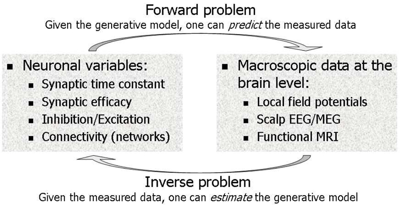
Generative models are biophysical models, which try to explain neuroimaging data (forward problem). The inverse problem consists of identifying the biophysical parameters of these models from the measured data. Dynamic Causal Modelling estimates the parameters of a given generative model (fMRI or MEG/EEG) using a Bayesian scheme.

In this review, the focus is on the formalism developed for Dynamic Causal Modelling (DCM) (David et al., 2006a; Friston et al., 2003; Garrido et al., 2007; Kiebel et al., 2006; Penny et al., 2004; Stephan et al., 2005). DCM is a generic approach for analysing for fMRI and EEG/MEG data using generative models. It imposes constraints on the mathematical structure of generative models so that they can be inverted easily using Bayesian estimation procedures. In brief, these models are usually deterministic input-output systems, which can be decomposed into a differential state equation and a nonlinear output or observer function. Following discussions which animated a workshop “Networks in Cognitive Systems/Trends and Challenges in Biomedicine: From Cerebral Process to Mathematical Tools Design” held at the Valparaiso Institute of Complex Systems in December 2006, I show here how this first generation of DCMs can be adapted to embed more autonomous modulatory mechanisms. The goal is to show that these models can be adapted to get closer to the self-organised and dissipative dynamics of living systems, as covered by formal theories used in biology such as autopoiesis (Varela et al., 1974). As an illustration, intracerebral EEG data, recorded in an epileptic patient during neurostimulation, will be used to illustrate how important questions about autonomous dynamics at the level of neuronal connections can be posed and addressed.

II. Dynamic Causal Modelling (DCM)

II.1. Concept

The main idea behind DCM (David et al., 2006a; Friston et al., 2003; Kiebel et al., 2006) is to treat the brain as a deterministic nonlinear dynamical system that is subject to inputs, and produces outputs. Effective connectivity, i.e. the influence that one region exerts on another, is parameterized in terms of coupling among unobserved brain states, i.e. neuronal activity in different regions. Coupling is estimated by perturbing the system and measuring the response. In other words, the principal aim of DCM is to explain evoked brain responses as deterministic responses to some perturbations, i.e. stimuli, in terms of context-dependent coupling, which allows for differences in the shape of responses. These perturbations elicit changes in unobserved neuronal activity simulated in neural networks, which is transformed into observed macroscopic neuroimaging data using a modality-specific forward model (Figure 2).

Figure 2.

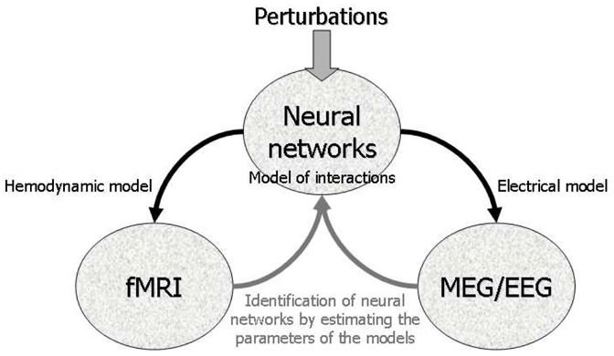
General concept of DCM. Brain activity is modelled with neural networks using a model of interactions (connectivity between different brain regions and/or neuronal populations). The neural states generate macroscopic data through a hemodynamic model for fMRI or an electrical model for MEG/EEG. The estimation of the parameters of the models allows one to estimate neuronal interactions, either from fMRI or from MEG/EEG. The fusion between fMRI/MEG/EEG data is implemented via the generative models at the level of neural networks.

DCM was developed first for fMRI (Friston et al., 2003) and can be used for any type of experimental design, as long as the data are acquired sequentially (DCM being a dynamical model, it necessitates continuous time-series). Here, the neuronal activity of each brain region participating in a DCM is summarised by one state variable, coined “synaptic activity”. Interactions between regions are modelled simply using a bilinear model that allows for input-dependent modulation of connectivity over time. This means that the neural dynamics generated are very simple (basically mono-exponential responses) and the relationships between real neuronal activity and modelled “synaptic activity” are quite obscure. However, it is not possible to estimate complicated neural dynamics from fMRI signals because they have intrinsically slow time constants (they can be considered as the output of a low-pass filter embodied by hemodynamic processes) and are sampled sparsely (every second or so, i.e. much slower than neural processes). The role of the neural model in DCM for fMRI is simply to estimate a summary of neural interactions, i.e. the strength of directed neuronal connections. The synaptic activity is estimated from the Blood Oxygenated Level Dependent (BOLD) signals by the means of a hemodynamic model (Friston et al., 2000) (Figure 3). The parameters of the hemodynamic model are estimated in each region to take into account spatial variability of hemodynamic responses. Inverting this model to estimate causal interactions at the neuronal level means the estimates are, in theory, not sensitive to this hemodynamic variability.

Figure 3.

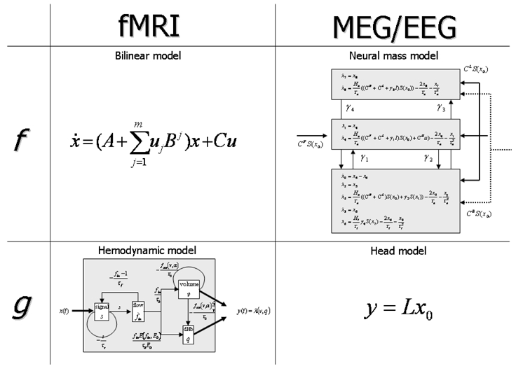
Schematic of the state equations f (Eq. 1) and output equations g (Eq. 2) used in fMRI and MEG/EEG. The state equation is more complex in MEG/EEG than in fMRI, whereas the output equation is simpler in MEG/EEG than in fMRI.

DCM for EEG relies on a neuronal model of interactions that is more plausible than the one used for fMRI. EEG signals are the macroscopic result of the activity of millions of neurons and DCMs for EEG use neural-mass models, which assume dynamics can be modelled by random fluctuations around population dynamics with a point mass (David and Friston, 2003). DCM for EEG has been developed as a generic tool to analyse evoked potentials obtained at the scalp level for any kind of neuropsychological or cognitive experiment. The generative model of DCM for EEG (David et al., 2005) is based on the Jansen model (Jansen and Rit, 1995), a neural-mass model developed originally for explaining visual responses. It is combined with rules of cortical-cortical connectivity derived from the analysis of connections between the different cortical layers in the visual cortex of the monkey (Crick and Koch, 1998). In the Jansen model, a cortical area, understood here as an ensemble of strongly interacting macro-columns, is modelled by a population of excitatory pyramidal cells, receiving (i) inhibitory and excitatory feedback from local (i.e. intrinsic) interneurons and (ii) excitatory input from neighbouring or remote (i.e. extrinsic) areas. It is composed of three subpopulations: a population of excitatory pyramidal (output) cells receives inputs from inhibitory and excitatory populations of interneurons, via intrinsic connections (intrinsic connections are confined to the cortical sheet). Within this model, excitatory interneurons can be regarded as spiny stellate cells found predominantly in layer four and in receipt of forward connections (Miller, 2003). Excitatory pyramidal cells and inhibitory interneurons are considered to occupy agranular layers and receive backward and lateral inputs. The resulting model (David et al., 2005) including intrinsic and extrinsic cortical-cortical connections, is a set of differential equations describing interactions between different inhibitory and excitatory neuronal populations (Figure 3). It can be specified easily to embed any hierarchical cortical-cortical network using forward, backward and lateral connections. The large cytoarchitectonic variability of the neocortex and of other brain structures such as the hippocampus and amygdala makes the plausibility of a generic model questionable. However, the crucial point here is that the main purpose of a forward model, in the context of DCM, is to constrain dynamics in a neuronally plausible way (time constants, propagation delay, directionality of the information transfer, etc.). This is exactly what a generic model can do, maintaining an appropriate balance between complexity, plausibility and modularity.

II.2. Theory

Because DCMs are not restricted to linear or instantaneous systems, they generally depend on a large number of free parameters. However, because they are biologically grounded, parameter estimation is constrained. A natural way to embody these constraints is within a Bayesian framework. Consequently, DCMs are estimated using Bayesian inversion and inferences about particular connections are made using their posterior or conditional density. The full set of equations for DCM specification and Bayesian parameter estimation can be found in the original papers (David et al., 2005; David et al., 2006a; Friston et al., 2003; Kiebel et al., 2006; Penny et al., 2004). The key steps are summarised below.

II.2.1. Model specification

A DCM is a dynamical system. It is specified in terms of a state equation and an output equation. The state equation can be written as

$$\stackrel{.}{x}=f(x,u,\theta )$$ (1)

where x are the neuronal states, u are the extrinsic inputs and θ are the model parameters. The output equation links the unobserved neuronal states x to the measured data y using a nonlinear instantaneous function g:

$$y=g(x,\theta ).$$ (2)

The equations (1) and (2) completely specify the forward model, that is how to link neuronal states x and their extrinsic perturbations u to the macroscopic data y. In other words, the functions f and g are specific to the modality used. In fMRI, f is fairly simple (because there is no information about detailed neural dynamics in BOLD signals) and approximates neuronal interactions with a bilinear model. The function g is much more complex, because it models the different biophysical processes at the origins of the BOLD effect: (i) the synaptic activity triggers a vasodilatory signal which induces changes in blood flow; (ii) according to the Balloon model (Buxton et al., 1998), changes in blood flow lead to changes in blood volume and in deoxyhemoglobin concentration. In comparison, in EEG, the f function is rather complex (nonlinear differential delayed equations) because one examine much richer neural dynamics than in fMRI. In contrast, the g function is extremely simple. It is the standard forward head model used for source localisation, namely a linear product of the pyramidal cell depolarisation (part of the hidden neural states, which are estimated via f) by the lead field of each region of the DCM. Figure 3 summarises the different equations. In fMRI, the parameters θ are the coupling parameters (connectivity) and hemodynamic parameters which control the dynamics of changes in blood flow, blood volume and deoxyhemoglobin content. For MEG/EEG, they are inhibitory and excitatory synaptic time constants and efficacies, intrinsic and extrinsic connectivity, and propagation delay.

II.2.2. Estimation of model parameters

DCM uses a Bayesian scheme for estimating model parameters based on Expectation-Maximisation (Friston et al., 2002). The outputs of the parameter estimation procedure are posterior probabilities of model parameters p(θ y) which are a combination of the likelihood (or confidence in the data) p(yθ) and prior expectations about the parameters (for example, synaptic time constants are expected to be around 5–10 ms) p(θ):

$$p(\theta \mid y)\propto p(y\mid \theta )p(\theta ).$$ (3)

Hyperparameters tune the relative influence of the data and of prior expectations. They are estimated from the data using a restricted Maximum Likelihood. The most important aspect is that inferences about the model parameters, and particularly about connectivity parameters, can be performed directly from the posterior distribution of those parameters (under Gaussian assumptions, one estimates and uses the conditional or posterior mean and covariance of the parameters).

II.2.3. Model comparison

The main advantage of DCM is that is allows one to test competing functional hypotheses. For each functional hypothesis, a model m is specified in terms of anatomical connections between regions and possibly the modulation of some connections by experimental context. This is equivalent to constructing a specific function f (Eq. 1) for each model. After the estimation of parameters of each competing model, the models are compared to find the most plausible model, or functional hypothesis. This is done using Bayesian model selection where the evidence of each model is used to quantify the model plausibility (Penny et al., 2004). The evidence of model m is given by

$$\begin{array}{l}p(y\mid m)=\int p(y\mid \theta ,m)p(\theta ,m)\propto p(y\mid \theta )d\theta \\ log(p(y\mid m))=\mathit{accuracy}(m)-\mathit{complexity}(m).\end{array}$$ (4)

The log-evidence can be decomposed into a difference between two components: an accuracy term, which quantifies the data fit, and a complexity term, which penalizes models with a large number of parameters. Therefore, the evidence embodies the two conflicting requirements of a good model, that it explains the data and is as simple as possible. The most likely model is the one with the largest log-evidence. Conventionally, strong evidence in favour of one model requires the difference in log-evidence to be three or more with other models.

Assuming each data set is independent of the others, the best model at the group level is obtained by multiplying the marginal likelihoods or equivalently, by adding the log-evidences from each subject (Garrido et al., 2007):

$$lnp(y_1,\dots ,y_n\mid m)=\sum _{j=1}^{n}lnp(y_j\mid m)$$ (5)

where n is the number of subjects. Note that the evidence can only be approximated under some assumptions. To obtain a consistent model comparison, one can use the Akaike Information Criterion (AIC) or the Bayesian Information Criterion (BIC) (Penny et al., 2004) to get bounds on the evidence and to select a model if the inference obtained with AIC and BIC is concordant.

III. Autopoietic systems

Autopoietic theory, or autopoiesis, is a formal attempt to describe living systems as physical open (dissipative) systems, but with a degree of autonomy (Varela, 1979). Autonomy is a general framework to understand their fundamental organisation. It is particularly useful when considering the individuality of living systems at different scales. It relies on circular causality (Figure 4), which is the central aspect of an autopoietic system (Letelier et al., 2003; Maturana and Varela, 1980):

Figure 4.

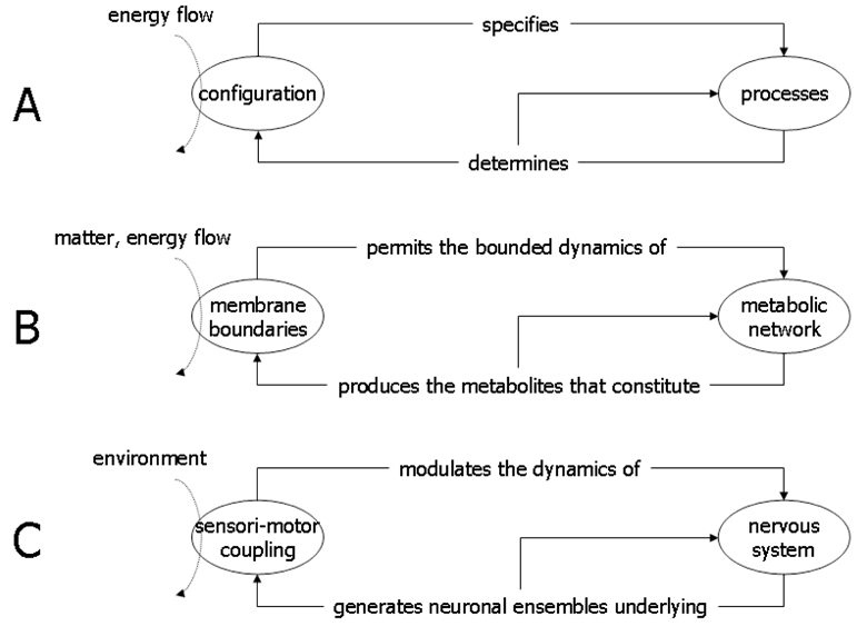
Partial representation of an autopoietic system at different scales: (A) Abstract level; (B) Cellular level; (C) Animal body level. The diagrams show the circular causality, or operational closure, which defines the autonomy of living systems. The system configuration (membrane boundaries/sensori-motor coupling) specifies a network of processes (metabolic network/nervous system) which in turn determines the system configuration or the dynamics of similar processes. Modified from (Rudrauf et al., 2003).

“an autopoietic system is organised as a bounded network of processes of production, transformation and destruction of components which (i) through their interactions and transformations continuously regenerate and realise the network of processes that produced them; (ii) constitute the system as a concrete entity in the space in which the components exist by specifying the topological realisation of the system as such a network”.

In other words, an autopoietic system produces a unity that is topographically and functionally segregated from its background. The operational closure (processes which produce components that are reinserted in the original processes by the means of other processes) of autopoietic systems is a general principle of organisation, which can be applied in many contexts; such as ecosystems, artificial intelligence and artificial life, social sciences, linguistics, economics and so on. In fact, autopoietic systems are a special case of a larger class of organisationally closed systems (Varela, 1979). This class includes (M,R) systems (Letelier et al., 2003; Rosen, 1958).

It is clear that the formalisms of DCM and autonomous systems such as autopoietic systems are not very different. The next section addresses their connections. This will lead to a simple modification of the standard DCMs to allow deterministic autonomous activity to be generated from perturbations, thus including autopoietic systems in the formalism of DCM.

IV. DCM and autopoietic systems

In neurodynamics, there are two classes of effects: dynamic effects and structural effects (David et al., 2006b). The distinction arises from a simple view of neuronal responses, as the response of an input-state-output system, such as a DCM defined by Eq. (1–2), to perturbations. From Eq. (1), it is immediately clear that the states x, and implicitly the system’s response y, can only be changed by perturbing the extrinsic inputs u or the parameters, θ. We refer to these as dynamic and structural effects respectively. This distinction arises in a number of different contexts. From a purely dynamical point of view, transients elicited by dynamic effects are the systems response to input changes; for example, presentations of a stimulus in an Event Related Potential (ERP) study. The duration and form of the resulting dynamic effect depends on the dynamical stability of the system to perturbations of its states (i.e. how the systems trajectories change with the state). Structural effects depend on structural stability (i.e. how the systems trajectories change with the parameters). Systematic changes in the parameters can produce systematic changes in the response, even in the absence of input. For systems that show autonomous (i.e. periodic or chaotic) dynamics, changing the parameters is equivalent to changing the attractor manifold, which induces a change in the systems states (Breakspear et al., 2003; Friston, 1997). For systems with fixed points and Volterra kernels, changing the parameters is equivalent to changing the kernels and transfer functions. This changes the spectral density relationships between the inputs and outputs. As such, structural effects are clearly important in the genesis of induced oscillations because they can produce frequency modulation of ongoing activity that does not entail phase-locking to any event. More generally, they play a critical role in short-term plasticity mechanisms observed in neuroimaging, for instance subject’s habituation after repetitive stimulation. Activity-dependent changes in synaptic activity are an important example of a structural effect that is induced by dynamic effects. This coupling of structural and dynamic mechanisms is closely related to the circular causality that characterises autopoietic systems. In fact, we will focus in activity or time-dependent changes in connectivity in the empirical example later.

At the neurobiological level, the distinction between dynamic and structural inputs speaks immediately to the difference between drivers from modulators (Sherman and Guillery, 1998). In sensory systems, a driver ensemble can be identified as the transmitter of receptive field properties. For instance, neurons in the lateral geniculate nuclei drive primary visual area responses, in the cortex, so that retinotopic mapping is conserved. Modulatory effects are expressed as changes in certain aspects of information transfer, by the changing responsiveness of neuronal ensembles in a context-sensitive fashion. A common example is attentional gain. Other examples involve extra-classical receptive field effects that are expressed beyond the classical receptive field. Generally, these are thought to be mediated by backward and lateral connections. In terms of synaptic processes, it has been proposed that the post-synaptic effects of drivers are fast (e.g. ionotropic receptors), whereas those of modulators are slower and more enduring (e.g. metabotropic receptors). The mechanisms of action of drivers refer to classical neuronal transmission, either biochemical or electrical, and are well understood. Conversely, modulatory effects can engage a complex cascade of highly nonlinear cellular mechanisms (Turrigiano and Nelson, 2004). Modulatory effects can be understood as transient departures from homeostatic states, lasting hundreds of milliseconds, due to synaptic changes in the expression and function of receptors and intracellular messaging systems. Classical examples of modularity mechanisms involve voltage-dependent receptors, such as NMDA receptors. These receptors do not cause depolarisation directly (i.e. a dynamic effect) but change the units sensitivity to depolarisation (i.e. a structural effect).

In short, the distinction between deterministic input-output systems, such as DCMs, and autonomous systems as formulated in theories such as autopoiesis and (M,R) systems is how dynamic and structural effects are instantiated and how they are coupled. In the standard interpretation, an autopoietic system creates an autonomous web of (molecular) processes that maintain autopoietic self-organisation (c.f., self-assembly in chemical systems). This means that it does not have structural inputs. In other words, the environment does not define the internal dynamics. The environment only perturbs the system’s dynamics. Here, there is no distinction between DCMs and autopoietic systems: both receive dynamic inputs, which act as transient perturbations. However, in autopoietic systems, the dynamic inputs trigger internal changes, or structural effects, which are defined by the very organisation of the autopoietic system itself. In contradistinction, the current formulation of DCM does not specify such operational closure. Instead, structural changes are specified as explicit and direct consequences of particular dynamic inputs. For instance, the changes in the dynamics of a DCM are usually defined by the modulation of interregional effective connectivity by an external modulatory input (i.e. the bilinear term in fMRI or the distinction between experimental conditions in MEG/EEG). Therefore, there is no operational closure; in the sense that an extrinsic input has to be added to initiate structural effects.

However, the operational closure of autopoietic systems is simple to specify in the context of DCM. In abstract form, the internal processes which realise transient structural modifications, triggered by dynamic input, can be defined as a generalised convolution

$$\theta =h(\stackrel{\sim }{x},\stackrel{\sim }{\theta })$$ (6)

where h can be any function and x̃ and θ̃ are the past history of the neuronal states x (in autopoietic terms: network of processes) and parameters θ (in autopoietic terms: molecular configuration). In summary, autopoietic systems can be defined operationally with a small set of equations, which extend the analytical formalism of DCM:

$$\begin{array}{l}\stackrel{.}{x}=f(x,u,\theta )\\ \theta =h(\stackrel{\sim }{x},\stackrel{\sim }{\theta })\\ y=g(x,\theta ).\end{array}$$ (7)

The two first equations embed operational closure: perturbations u initiate changes in the states (processes) x that depend on the parameters θ (configuration). In return, the system’s configuration, or structure, is a function of the history of its configuration and of its processes. This is the basis of an autonomous system, which generates intrinsic structural changes triggered by external inputs. The last equation is simply the output equation through which the states of the system are transformed into measurable variables y. In neuroimaging, these are the BOLD signals and scalp MEG/EEG. Figure 5 places Eq. (7) into an autopoietic scheme.

Figure 5.

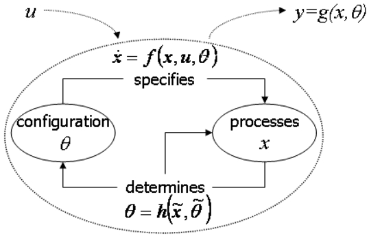
Autopoietic interpretation of Eq. (7). The parameters θ play the role of the configuration. The processes are the neural states x. They are specified by the state equation f and their past history and the past history of the parameters. In turn, these determine a new configuration using the function h. Perturbations u is the equivalent of energy inflow. The macroscopic data y are the output of an observer equation g; hence they do not play an explicit role in the intrinsic dynamics of the system.

Now that the formalism of a DCM for autopoietic systems has been established, we will test the face-validity of this approach using experimental data from deep brain stimulation in an epileptic patient. We will then discuss the benefits of including autonomous dynamics in the context of DCM in comparison to its standard formulation.

V. An illustration: short-term plasticity during pre-surgical neurostimulation

Epilepsy is a common chronic neurological disorder characterised by recurrent spontaneous epileptic seizures. A cortical imbalance between excitatory and inhibitory mechanisms is likely to be the pathophysiological basis for human partial epilepsy. In addition to long-lasting susceptibility to epileptic discharges, transient modifications of neural networks properties, such as those induced by electrical stimulation, can also lead to the occurrence of epileptic events in patients (Chauvel et al., 1993; Kahane et al., 1993; Kahane et al., 2004; Kalitzin et al., 2005; Schulz et al., 1997; Valentin et al., 2002; Wilson et al., 1998). In particular, several studies have noted that short-term plasticity of evoked responses (Wilson et al., 1998; Wozniak et al., 2007) or of oscillatory responses (Kalitzin et al., 2005) is induced easily by repetitive stimulations in the epileptic regions, without causing a systematic seizure. Knowing whether these fast changes in evoked responses conform to autonomous dynamics is an important issue which can be addressed explicitly by the theoretical considerations of the previous section.

The full description of the clinical and scientific context of pre-surgical neurostimulation and of our data acquisition protocol and patient characteristics can be found elsewhere (David et al., in preparation; Wozniak et al., in preparation). Here we summarise those elements needed to understand the DCM treatment. The patient included in this study was suffering from temporal lobe epilepsy. She had been selected for resective surgery and had undergone standard pre-surgical clinical evaluations, including 1 Hz intracerebral electrical stimulation (Kahane et al., 1993; Kahane et al., 2004). The patient was fully informed and gave her consent before being implanted and stimulated. Intracerebral recordings were performed using an audio-video-EEG monitoring system (Micromed, Treviso, Italy) that recorded up to 128 contacts simultaneously, so that a large range of mesial and cortical areas were sampled. Stimulation at 1 Hz (pulse width 3 milliseconds) was applied to the amygdala between two contiguous contacts. The goals of the stimulation were the reproduction of the aura, the induction of an electro-clinical seizure, and/or the localization of eloquent cortical areas to be spared during surgery. Bipolar stimuli were delivered using a constant current rectangular pulse generator designed for a safe diagnostic stimulation of the human brain, using parameters proved to produce no structural damage. The intensity used was 3mA. Stimulation lasted 34 seconds (34 brief stimulations) and evoked responses were recorded in the amygdala, anterior hippocampus, temporal pole and fusiform gyrus. After stimulation 25, some irregular spiking and fast oscillations were observed reflecting the electro-clinical signs of the forthcoming seizure. The first clinical symptoms occurred around stimulation 31 (i.e., after 31 seconds). The anterior hippocampus was the candidate for an epileptic focus and short-term plasticity was expressed most in this structure (Figure 6).

Figure 6.

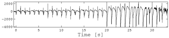
Evoked responses in the anterior hippocampus during 1Hz stimulation of the amygdala. Note the increasing amplitude of responses up to stimulation 25 (24 s). After stimulation 25, responses become irregular with fast activity indicating a non-physiological (epileptic) behaviour.

For simplicity, we isolated the anterior hippocampus for a DCM study and modelled it with a cortical macro-column composed of inhibitory and excitatory neuronal populations (Jansen and Rit, 1995). The Jansen model is certainly not the optimal neuronal model for the anterior hippocampus but the objective was not to detail the activity of the perforant pathway, dentate gyrus, CA1, CA2, CA3 and so on. The Jansen model is simply a way to summarise the complex neuronal interactions in a neural mass model that captures the basic dynamics of observed macroscopic EEG. Isolating the hippocampus from the rest of the brain imposes formal topological constrains which do not necessarily exist (the hippocampus is embedded in more extended neural networks). However, it allows us to deal with a simple neural model, in which all inputs from other stimulated regions (direct connections with the amygdala but also potential relay with other structures, see (David et al., in preparation) for a more complete analysis) are pooled under a single exogenous input. This means we made the implicit assumption that the anterior hippocampus is an autonomous system, itself nested in a bigger system (the brain, or the human body, or society, or the universe). This is justified by the fact that neural activity can be recorded in hippocampal slices in vitro.

To explain the changes of hippocampal responses y shown in Figure 6, we considered the following competing models or hypotheses (Figure 7):

Figure 7.

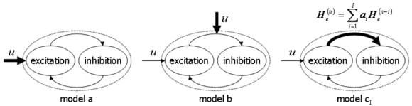
The different DCMs of the hippocampus tested to explain the data shown in Figure 6. The bold arrows correspond to the modulated connections. Models a and b are standard DCMs. Models c_I incorporates autonomous dynamics on the parameters. Note that the loop between excitation and inhibition captures the concept of interactions between excitatory and inhibitory neuronal populations but does not exactly reflect the architecture of the Jansen model (see Fig. 3).

1. Model a: Changes in y (responses) are a direct consequence of changes in u (input). In other words, plasticity has been expressed outside the hippocampus by neural networks linking the amygdala to the hippocampus (monosynaptic or polysynaptic connections). In this model we modelled a different input strength for each stimulation.

2. Model b: Input u is stable over stimulations and short-term plasticity observed in y corresponds to a modulation of the excitatory efficacy of intrinsic connections within the hippocampus, the dynamics of which are set by an exogenous modulatory input. This is a structural mechanism explained within the standard formulation of DCM (Eq. 1–2). In this model there are two inputs; a dynamic input, which is now fixed for each stimulation and a structural input that changed the connectivity and is specific to each stimulation.

3. Model c: Input u is stable over stimulations and short-term plasticity observed in y corresponds to an autonomous modulation of excitatory efficacy of intrinsic connections within the hippocampus. This corresponds to an autonomous DCM (Eq. 7). Here, we consider a simple linear autoregressive model for the structural dynamics concerning excitatory synaptic efficacies. Thus the structural input of model b is replaced by Eq. (6) which reduces to:

   $$H_e^{(n)}=\sum _{i=1}^I{a}_i{H}_e^{(n-i)}$$ (8)

   where $H_e^{(n)}$ is the excitatory synaptic efficacy at stimulation n and I is the model order; in other words, the horizon below which past activity has an effect on the current structure. This model has fewer parameters than the preceding models because the number of autoregression coefficients is less than the number of stimulations. However, as we will see below it can model equally, if not more, complex dynamics. Besides knowing whether model c can explain the stimulation-induced dynamics, the size of the memory effect in the autonomous dynamics is itself interesting, i.e. what is the most plausible I. To assess this, we performed a Bayesian model comparison among the models constructed for each value of I between 1 and N−1 (N=25 is the maximal number of stimulations before the beginning of epileptic activity). Each model is noted model c_I.

The parameters for each model were estimated from the data y shown in Figure 6. Pre-processing comprised: (i) band-pass filtering between 5 and 40 Hz and (ii) concatenation of the first 25 evoked responses between 0 and 150ms. The results are shown in Figure 8. On comparing the log-evidences of the different models, it transpired that model a is the most likely. Indeed, this model reproduces the observed time series with a remarkable fidelity. This suggests that the time-dependent responses, expressed in the anterior hippocampus, are most probably due to changes in its extrinsic inputs (or changes in sensitivity to inputs as mediated by the modulation of the expression of NMDA receptors). One point is important to stress when looking the time series of model b (and of c1 and c10): the changes in synaptic efficacies are related directly to the maximum amplitude of evoked responses, and are therefore highly correlated with the extrinsic input in model a. However, model b fits the first positive component of the evoked responses well but not the second negative component. In fact, the excitatory efficacy has an effect not only on the amplitude of responses but also on their shape and, implicitly, their frequency content. Because model a, which estimates an excitatory efficacy over stimulations, is able to fit the data for any kind of response amplitude, these results suggest that the efficacy of connections intrinsic to the hippocampus is more or less constant. This is the main reason why model a is much more plausible than the others. To conclude, the first interesting aspect of this DCM analysis is that the short-term changes in hippocampal responses to stimulation of the amygdala are more likely to be caused by plasticity in effective connectivity between the hippocampus and other brain regions, as opposed to some modulation of intrinsic hippocampal susceptibility. This calls for a DCM analysis extended to other brain regions, which can be found in (David et al., in preparation).

Figure 8.

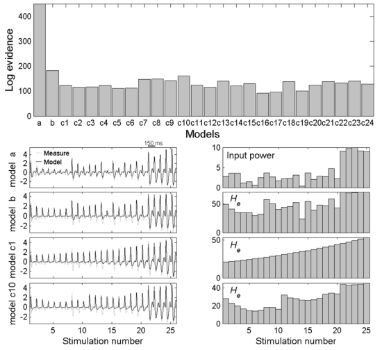
On top, the log-evidences (under BIC assumption) of the different models clearly shows that model a is the most plausible. Model b ranks second. Among “autonomous” models, model c₁₀ is the best. Below, on the left hand side, time series are shown (original: grey, adjusted: black) for models a, b, c₁ and c₁₀. Corresponding variables modulated over stimulations (input power for model a, excitatory synaptic efficacy for models b, c₁ and c₁₀) are shown on the right hand side.

Nonetheless, let us continue the discussion of the results by focusing on model b and its autonomous formulation (models c). We will describe the constraints and the advantages of using an autonomous formulation of a DCM. For models c, the log-evidences indicate that model c₁₀ is the most plausible, given the data. This corresponds to a model order of ten, for the autoregressive evolution of synaptic efficacy. For comparison, we show in Figure 8 the time series for this model and also those for the simplest model (model c₁). Both models show a gradual increase in excitatory efficacy with the repetition of the stimulation. The dynamics generated are very simple (monotonous) for model c₁ and fairly more complex for model c₁₀, where a pattern lasting ten stimulations is repeated approximately. In other words, there is a constraint on the model dynamics, which is given by the structural equation (Eq. 6 or 8). If this is too strict the model will not adjust to the data in comparison to when there is no such constraint (model b).

Results obtained with models a and b were very interesting because they showed it was possible to track the evolution of the extrinsic input to, or of the excitatory synaptic efficacy within, the hippocampus. Besides the ability to reproduce data, a good model is also characterised by its ability to make predictions. For models a and b, this is no prediction because these models have no autopoietic memory. In contradistinction, predictions can be made with an “autonomous DCM” because there is an explicit modelling of the rate of changes of structural effects over time; this generates autonomous structural dynamics, which has consequences for neural responses. The visual inspection of the evolution for models c₁ and c₁₀ shows the inertia of the autonomous dynamics characterised by the autoregressive model. It is easy to imagine that the system will continue to diverge if the stimulations were to be repeated ad vitam eternam. This is exactly what we have simulated in Figure 9 for model c₁₀: we added two stimulations (stimulations 26 and 27) and let the system predict the dynamics. According to the parameters of the autoregressive model estimated from previous stimulations, the DCM predicted an increase of excitatory efficacy as expected from Figure 8. The corresponding time series are somewhat more interesting: they show a catastrophic divergence, indicating that the Jansen model is approaching a phase-transition or bifurcation. More precisely, the system manifold is no longer a mass point attractor centred on zero. One might interpret this as the hippocampus entering an epileptic regime because of an increase of excitatory efficacy, which is what actually happened. The fascinating aspect is that the autonomous DCM has estimated, from the pre-ictal regime, a set of excitatory efficacies at the limit of the point of bifurcation between a stable and divergent dynamics. This indicates that physiological brain dynamics could be at the limit of stability and particularly prone to generate oscillations and complex nonlinear dynamical behaviours such as chaotic itinerancy (Tsuda, 2001) and epileptic seizures in pathological circuits.

Figure 9.

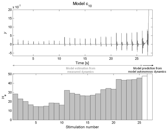
When adding (artificial) additional stimulations, the parameters of model c₁₀ predict an increase of excitatory efficacy (white bars). This corresponds to diverging responses, which can be interpreted as the beginning of an induced seizure. This is a prediction which is possible only because structural changes are specified autopoietically within the model.

VI. Conclusion

This review attempts a synthesis, in simple terms, of two important conceptual frameworks: Dynamic Causal Modelling (Friston et al., 2003) and the theory of autopoietic systems (Varela et al., 1974). DCM has been developed recently by the neuroimaging community to explain, using biophysical models, how fMRI/MEG/EEG data are related to neural processes. The classical approach in neuroimaging is to explore a data set with the following question: Where is a given processes implemented in the brain? Standard statistical maps are then constructed to reveal regional effects and various statistical tests can be performed to establish the regional specificity of different experimental manipulations. DCM goes further by asking: How are they responses implemented in mechanistic terms? This question represents the opportunity to rethink the design of cognitive experiments in functional neuroimaging and to appreciate the underlying neural mechanisms. The parameters of biophysical models are estimated from the measured data. Different functional hypotheses can therefore be tested explicitly. DCM represents a relevant biophysical approach to exploring brain data with a potential, which has yet to be fully evaluated.

Since the 1970s, autopoiesis and related formal theories of living systems as autonomous machines has had many successful applications in various arenas outside biology (Letelier et al., 2003). But autopoiesis, though acclaimed by theorists in many disciplines (Mingers, 1995), has had a limited practical impact because of the difficulties applying theoretical ideas, such as wholeness, to experimental data. Here, we have tried to disclose the connections between DCM and autopoiesis. In particular, we have proposed a simple modification to the standard formulation of DCM that accommodates a simple model of autonomy. The idea was to exploit the inferential machinery of the system identification with DCMs in neuroimaging to test the face validity of the autopoietic theory applied to neural subsystems. This exciting field of research is still essentially unexplored and we hope to have advanced the feasibility of this approach.

References

- Attwell D, Iadecola C. The neural basis of functional brain imaging signals. Trends Neurosci. 2002;25:621–625. doi: 10.1016/s0166-2236(02)02264-6. [DOI] [PubMed] [Google Scholar]
- Breakspear M, Terry JR, Friston KJ. Modulation of excitatory synaptic coupling facilitates synchronization and complex dynamics in a biophysical model of neuronal dynamics. Network. 2003;14:703–732. [PubMed] [Google Scholar]
- Buxton RB, Wong EC, Frank LR. Dynamics of blood flow and oxygenation changes during brain activation: the balloon model. Magn Reson Med. 1998;39:855–864. doi: 10.1002/mrm.1910390602. [DOI] [PubMed] [Google Scholar]
- Chauvel P, Landre E, Trottier S, Vignel JP, Biraben A, Devaux B, Bancaud J. Electrical stimulation with intracerebral electrodes to evoke seizures. Adv Neurol. 1993;63:115–121. [PubMed] [Google Scholar]
- Crick F, Koch C. Constraints on cortical and thalamic projections: the no-strong-loops hypothesis. Nature. 1998;391:245–250. doi: 10.1038/34584. [DOI] [PubMed] [Google Scholar]
- Dale AM, Liu AK, Fischl BR, Buckner RL, Belliveau JW, Lewine JD, Halgren E. Dynamic statistical parametric mapping: combining fMRI and MEG for high-resolution imaging of cortical activity. Neuron. 2000;26:55–67. doi: 10.1016/s0896-6273(00)81138-1. [DOI] [PubMed] [Google Scholar]
- David O, Friston KJ. A neural mass model for MEG/EEG: coupling and neuronal dynamics. Neuroimage. 2003;20:1743–1755. doi: 10.1016/j.neuroimage.2003.07.015. [DOI] [PubMed] [Google Scholar]
- David O, Harrison L, Friston KJ. Modelling event-related responses in the brain. Neuroimage. 2005;25:756–770. doi: 10.1016/j.neuroimage.2004.12.030. [DOI] [PubMed] [Google Scholar]
- David O, Kiebel SJ, Harrison LM, Mattout J, Kilner JM, Friston KJ. Dynamic causal modeling of evoked responses in EEG and MEG. Neuroimage. 2006a;30:1255–1272. doi: 10.1016/j.neuroimage.2005.10.045. [DOI] [PubMed] [Google Scholar]
- David O, Kilner JM, Friston KJ. Mechanisms of evoked and induced responses in MEG/EEG. Neuroimage. 2006b;31:1580–1591. doi: 10.1016/j.neuroimage.2006.02.034. [DOI] [PubMed] [Google Scholar]
- David O, Wozniak A, Minotti L, Kahane P. Preictal short-term plasticity induced by intracerebral 1 Hz stimulation: II. Dynamic Causal Modelling. doi: 10.1016/j.neuroimage.2007.11.005. in preparation. [DOI] [PubMed] [Google Scholar]
- Friston KJ. Transients, metastability, and neuronal dynamics. Neuroimage. 1997;5:164–171. doi: 10.1006/nimg.1997.0259. [DOI] [PubMed] [Google Scholar]
- Friston KJ, Harrison L, Penny W. Dynamic causal modelling. Neuroimage. 2003;19:1273–1302. doi: 10.1016/s1053-8119(03)00202-7. [DOI] [PubMed] [Google Scholar]
- Friston KJ, Mechelli A, Turner R, Price CJ. Nonlinear responses in fMRI: the Balloon model, Volterra kernels, and other hemodynamics. Neuroimage. 2000;12:466–477. doi: 10.1006/nimg.2000.0630. [DOI] [PubMed] [Google Scholar]
- Friston KJ, Penny W, Phillips C, Kiebel S, Hinton G, Ashburner J. Classical and Bayesian inference in neuroimaging: theory. Neuroimage. 2002;16:465–483. doi: 10.1006/nimg.2002.1090. [DOI] [PubMed] [Google Scholar]
- Garrido MI, Kilner JM, Kiebel SJ, Stephan KE, Friston KJ. Dynamic causal modelling of evoked potentials: A reproducibility study. Neuroimage. 2007 doi: 10.1016/j.neuroimage.2007.03.014. [DOI] [PMC free article] [PubMed] [Google Scholar]
- Hamalainen M, Hari R, Ilmoniemi R, Knuutila J, Lounasmaa O. Magnetoencephalography. Theory, instrumentation and applications to tne noninvasive study of brain function. Rev Mod Phys. 1993;65:413–497. [Google Scholar]
- Jansen BH, Rit VG. Electroencephalogram and visual evoked potential generation in a mathematical model of coupled cortical columns. Biol Cybern. 1995;73:357–366. doi: 10.1007/BF00199471. [DOI] [PubMed] [Google Scholar]
- Kahane P, Minotti L, Hoffmann D, Lachaux J-P, Ryvlin P. Invasive EEG in the definition of the seizure onset zone: depth electrodes. In: Rosenow F, Lüders HO, editors. Handbook of Clinical Neurophysiology. Vol. 3. Elsevier BV; Amsterdam: 2004. pp. 109–133. [Google Scholar]
- Kahane P, Tassi L, Francione S, Hoffmann D, Lo RG, Munari C. Electroclinical manifestations elicited by intracerebral electric stimulation “shocks” in temporal lobe epilepsy. Neurophysiol Clin. 1993;23:305–326. doi: 10.1016/s0987-7053(05)80123-6. [DOI] [PubMed] [Google Scholar]
- Kalitzin S, Velis D, Suffczynski P, Parra J, da Silva FL. Electrical brain-stimulation paradigm for estimating the seizure onset site and the time to ictal transition in temporal lobe epilepsy. Clin Neurophysiol. 2005;116:718–728. doi: 10.1016/j.clinph.2004.08.021. [DOI] [PubMed] [Google Scholar]
- Kiebel SJ, David O, Friston KJ. Dynamic causal modelling of evoked responses in EEG/MEG with lead field parameterization. Neuroimage. 2006;30:1273–1284. doi: 10.1016/j.neuroimage.2005.12.055. [DOI] [PubMed] [Google Scholar]
- Letelier JC, Marin G, Mpodozis J. Autopoietic and (M,R) systems. J Theor Biol. 2003;222:261–272. doi: 10.1016/s0022-5193(03)00034-1. [DOI] [PubMed] [Google Scholar]
- Logothetis NK, Wandell BA. Interpreting the BOLD signal. Annu Rev Physiol. 2004;66:735–769. doi: 10.1146/annurev.physiol.66.082602.092845. [DOI] [PubMed] [Google Scholar]
- Maturana H, Varela F. Autopoiesis and cognition: The realization of the living. Reidel; Dordrecht: 1980. [Google Scholar]
- Miller KD. Understanding layer 4 of the cortical circuit: a model based on cat V1. Cereb Cortex. 2003;13:73–82. doi: 10.1093/cercor/13.1.73. [DOI] [PubMed] [Google Scholar]
- Mingers J. Self-producing systems: Implications and applications of autopoiesis. Plenum Press; New York: 1995. [Google Scholar]
- Nunez PL, Srinivasan R. Electric fields of the brain. 2. Oxford University Press; New York: 2005. [Google Scholar]
- Penny W, Stephan K, Mechelli A, Friston K. Comparing dynamic causal models. Neuroimage. 2004 doi: 10.1016/j.neuroimage.2004.03.026. [DOI] [PubMed] [Google Scholar]
- Poznanski RR, Riera JJ. fMRI models of dendritic and astrocytic networks. J Integr Neurosci. 2006;5:273–326. doi: 10.1142/s0219635206001173. [DOI] [PubMed] [Google Scholar]
- Riera JJ, Jimenez JC, Wan X, Kawashima R, Ozaki T. Nonlinear local electrovascular coupling. II: From data to neuronal masses. Hum Brain Mapp. 2006a doi: 10.1002/hbm.20278. [DOI] [PMC free article] [PubMed] [Google Scholar]
- Riera JJ, Wan X, Jimenez JC, Kawashima R. Nonlinear local electrovascular coupling. I: A theoretical model Hum Brain Mapp. 2006b;27:896–914. doi: 10.1002/hbm.20230. [DOI] [PMC free article] [PubMed] [Google Scholar]
- Riera JJ, Watanabe J, Kazuki I, Naoki M, Aubert E, Ozaki T, Kawashima R. A state-space model of the hemodynamic approach: nonlinear filtering of BOLD signals. Neuroimage. 2004;21:547–567. doi: 10.1016/j.neuroimage.2003.09.052. [DOI] [PubMed] [Google Scholar]
- Robinson PA, Rennie CJ, Wright JJ, Bahramali H, Gordon E, Rowe DL. Prediction of electroencephalographic spectra from neurophysiology. Phys Rev E. 2001;63:021903. doi: 10.1103/PhysRevE.63.021903. [DOI] [PubMed] [Google Scholar]
- Rosen R. A relational theory of biological systems. Bull Math Biophys. 1958;20:245–341. [Google Scholar]
- Rudrauf D, Lutz A, Cosmelli D, Lachaux JP, Le Van QM. From autopoiesis to neurophenomenology: Francisco Varela’s exploration of the biophysics of being. Biol Res. 2003;36:27–65. doi: 10.4067/s0716-97602003000100005. [DOI] [PubMed] [Google Scholar]
- Schulz R, Luders HO, Tuxhorn I, Ebner A, Holthausen H, Hoppe M, Noachtar S, Pannek H, May T, Wolf P. Localization of epileptic auras induced on stimulation by subdural electrodes. Epilepsia. 1997;38:1321–1329. doi: 10.1111/j.1528-1157.1997.tb00070.x. [DOI] [PubMed] [Google Scholar]
- Sherman SM, Guillery RW. On the actions that one nerve cell can have on another: distinguishing “drivers” from “modulators”. Proc Natl Acad Sci USA. 1998;95:7121–7126. doi: 10.1073/pnas.95.12.7121. [DOI] [PMC free article] [PubMed] [Google Scholar]
- Stephan KE, Harrison LM, Penny WD, Friston KJ. Biophysical models of fMRI responses. Curr Opin Neurobiol. 2004;14:629–635. doi: 10.1016/j.conb.2004.08.006. [DOI] [PubMed] [Google Scholar]
- Stephan KE, Penny WD, Marshall JC, Fink GR, Friston KJ. Investigating the functional role of callosal connections with dynamic causal models. Ann NY Acad Sci. 2005;1064:16–36. doi: 10.1196/annals.1340.008. [DOI] [PMC free article] [PubMed] [Google Scholar]
- Tsuda I. Toward an interpretation of dynamic neural activity in terms of chaotic dynamical systems. Behav Brain Sci. 2001;24:793–810. doi: 10.1017/s0140525x01000097. [DOI] [PubMed] [Google Scholar]
- Turrigiano GG, Nelson SB. Homeostatic plasticity in the developing nervous system. Nat Rev Neurosci. 2004;5:97–107. doi: 10.1038/nrn1327. [DOI] [PubMed] [Google Scholar]
- Valentin A, Anderson M, Alarcon G, Seoane JJ, Selway R, Binnie CD, Polkey CE. Responses to single pulse electrical stimulation identify epileptogenesis in the human brain in vivo. Brain. 2002;125:1709–1718. doi: 10.1093/brain/awf187. [DOI] [PubMed] [Google Scholar]
- Varela F. Principles of biological autonomy. Elsevier; North Holland, New York: 1979. [Google Scholar]
- Varela FG, Maturana HR, Uribe R. Autopoiesis: the organization of living systems, its characterization and a model. Curr Mod Biol. 1974;5:187–196. doi: 10.1016/0303-2647(74)90031-8. [DOI] [PubMed] [Google Scholar]
- Vazquez AL, Cohen ER, Gulani V, Hernandez-Garcia L, Zheng Y, Lee GR, Kim SG, Grotberg JB, Noll DC. Vascular dynamics and BOLD fMRI: CBF level effects and analysis considerations. Neuroimage. 2006;32:1642–1655. doi: 10.1016/j.neuroimage.2006.04.195. [DOI] [PubMed] [Google Scholar]
- Wilson CL, Khan SU, Engel J, Jr, Isokawa M, Babb TL, Behnke EJ. Paired pulse suppression and facilitation in human epileptogenic hippocampal formation. Epilepsy Res. 1998;31:211–230. doi: 10.1016/s0920-1211(98)00063-1. [DOI] [PubMed] [Google Scholar]
- Wozniak A, Minotti L, Kahane P, David O. Preictal short-term plasticity induced by intracerebral 1 Hz stimulation: I. Localisation of the seizure onset zone. doi: 10.1016/j.neuroimage.2007.11.005. in preparation. [DOI] [PubMed] [Google Scholar]