

Abstract
We propose a novel diffusion tensor imaging (DTI) registration algorithm, called Tensor Image Morphing for Elastic Registration (TIMER), which leverages the hierarchical guidance of regional distributions and local boundaries, both extracted directly from the tensors. Currently available DTI registration methods generally extract tensor scalar features from each tensor to construct scalar maps. Subsequently, regional integration and other operations such as edge detection are performed to extract more features to guide the registration. However, there are two major limitations with these approaches. First, the computed regional features might not reflect the actual regional tensor distributions. Second, by the same token, gradient maps calculated from the tensor-derived scalar feature maps might not represent the actual tissue tensor boundaries. To overcome these limitations, we propose a new approach which extracts regional and edge information directly from a tensor neighborhood. Regional tensor distribution information, such as mean and variance, is computed in a multiscale fashion directly from the tensors by taking into account the voxel neighborhood of different sizes, and hence capturing tensor information at different scales, which in turn can be employed to hierarchically guide the registration. Such multiscale scheme can help alleviate the problem of local minimum and is also more robust to noise since one can better determine the statistical properties of each voxel by taking into account the properties of its surrounding. Also incorporated in our method is edge information extracted directly from the tensors, which is crucial to facilitate registration of tissue boundaries. Experiments involving real subjects, simulated subjects, fiber tracking, and atrophy detection indicate that TIMER performs better than the other methods in comparison (Yang et al., 2008a; Zhang et al., 2006).
Keywords: Diffusion Tensor Imaging, Elastic Registration, Tensor Regional Distributions, Tensor Boundaries, Log-Euclidean Manifold
1. Introduction
Diffusion tensor imaging (DTI) is capable of non-invasively measuring water diffusion in vivo. While DTI has been widely employed to delineate potential white matter abnormality in different neurological diseases, registration of diffusion tensor images across different subjects is a critical prerequisite for detailed statistical analysis on voxel-by-voxel basis. However, spatial normalization of diffusion tensor images is challenging both technically and computationally given that tensor data representation is high dimensional in nature, and it is required that the tensors not only be spatially warped, but also be reoriented to appropriately reflect the anisotropic diffusivity.
In conventional MRI, such as T1– and T2– weighted images, white matter often appears as a homogeneous structure, even though it consists of many axonal bundles of various sizes and orientations. The advent of DTI makes deeper investigation into these structures possible (Huang et al., 2006; Lee et al., 2008; Liu et al., 2007; Yang et al., 2008b). It has been observed that water diffusivity is more restricted in the transverse direction of the axonal fibers in white matter tissue than along the axial direction. DTI takes advantage of this anisotropic diffusivity and measures a symmetric second order tensor at each voxel characterizing the anisotropy which provides two extra pieces of information regarding the material microstructure over simple diffusion weighted MRI (Alexander, 2006). First, it provides rotationally invariant statistics of the anisotropy of the particle displacement probability density function p. Second, it provides an estimate of the dominant orientation of microstructural fibres. Assuming Gaussian distribution, the shape of p is determined by the eigenvalues λ1 ≥ λ2 ≥ λ3 of tensor D. The Gaussian function has ellipsoidal contours, relative lengths of the major axes of which have the same proportions as . Statistics of anisotropy come from the distribution of eigenvalues. The principal direction (PD) of the tensor is presumed to coincide with the underlying fiber orientation. With fiber orientation information, one can identify various axonal tracts within the homogeneous-looking white matter. Therefore, DTI can provide unique microstructural and physiological insight into the white matter of brains, which has not been found available in other MR modalities, and has thus become a powerful technique for analyzing the underlying white matter structure of brains (Mori et al., 2001; Pierpaoli et al., 1996). The rich microstructural information of white matter facilitates the study of development, aging, and disease on specific white matter regions of interest.
To quantify diffusion tensor abnormalities based on voxel-based statistical analysis, spatial normalization is necessary in order to minimize the anatomical variability between studied brain structures. Conventional methods generally extract tensor scalar features from each tensor individually, and by constructing scalar maps, regional integration and other operations such as edge detection can be performed to extract final features for correspondence matching. As an example, Yang et al. (Yang et al., 2008a) capitalize on tensor structural geometry and orientation information for registration guidance. Specifically, geometric measures, describing the diffusion tensor geometrical resemblance to the generic structures of prolateness, oblateness, and sphericity (Westin et al., 1997), are computed for each voxel. The distributions of the measures in a spherical neighborhood of each voxel are then estimated using local histograms. These local histograms, together with boundary information extracted from the fractional anisotropy (FA) and apparent diffusion coefficient (ADC) maps are finally fed into a deformable correspondence matching mechanism (Shen, 2007) to align the images.
There are, however, two major limitations with these approaches. First, the computed regional features might not reflect the actual regional tensor distributions. Second, by the same token, gradient maps calculated from the tensor-derived scalar feature maps might not represent the actual tissue tensor boundaries. While it is possible to use the results of structural image registration to establish correspondence matching as required in the registration process, it is natural to expect that the inclusion of additional information within the diffusion tensor will lead to more accurate matching and hence more robust registration, particularly in white matter regions where the microstructural variation is not observable in previous conventional MRI based methods. In view of this, new approaches are proposed to work directly on the tensors. Methods involving single voxel correspondence matching can be susceptible to the effect of noise and also spurious variation of anatomical structures. A more robust approach is to leverage information gathered from the voxel neighborhood to help estimate better voxel statistics, so as to make correspondence matching less affected by noise.
In this paper, we propose a novel diffusion tensor image registration algorithm, called Tensor Image Morphing for Elastic Registration (TIMER). Instead of working with the tensors in a voxel-wise fashion, we estimate the statistical properties, such as mean and variance, at a particular voxel location by taking into consideration the information furnished by the voxel neighborhood. Notably, these regional information are obtained directly from the tensors and not their scalar maps. Scalar maps do not retain full tensor information as some information is discarded in the process of their computation, and hence they do not reflect true tensor stuctures. As a simple example, a homogeneous region on a FA map might contain tensors of radically different orientations and there is no way to tell the difference by solely gauging from the FA map, simply because the FA map does not hold orientation information. Computing regional distribution directly using the tensors take all these information into account and yields a more precise estimation of the statistical property at a particular voxel location. However, measures derived from tensor regional distributions in a single resolution are very limited in its discriminating power as in reality anatomical details often appear in different scales. This problem can be overcome by simply combining a set of regional features at multiple scales. Tensor regional information from each scale captures different spatial information and when combined forms a rich discriminative feature vector. It can be observed from Fig. 1 that regional information irrespective of the neighborhood size is not adequate for differentiating different anatomical structures, but by simply combining regional information gained from three different resolutions, we can sufficiently achieve differentiation.
Figure 1.
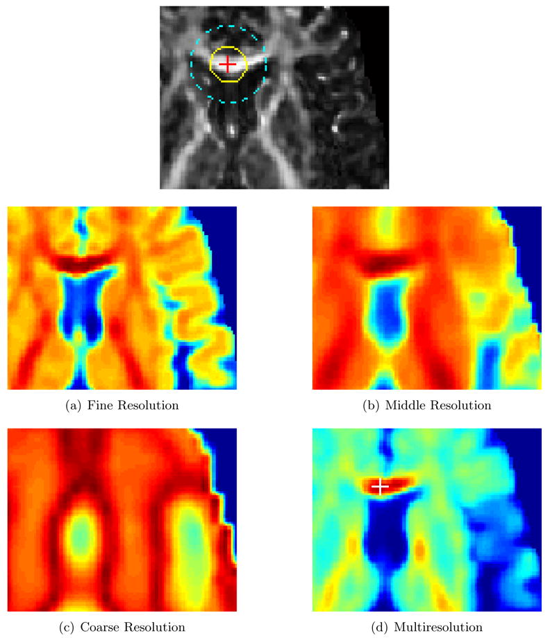
The principal diffusitivies of the mean in the neighborhood of the point indicated in the top image is compared with those of the other points in the brain image volume. Dark red indicates high similarity and dark blue indicates otherwise. (a), (b) and (c) are the results obtained at fine, middle and coarse resolution representations of the diffusion tensor image, respectively. (d) is the result when all the individual resolutions in (a), (b) and (c) are combined. The small delineated dark red area in (d) is indicative that a correspondence can be correctly located as opposed to (a), (b) and (c) where the dark red regions are spread out with no clear clue of where the corresponding point is. The white cross in (d) corresponds with the red cross in the top image.
It is worth noting that features captured from regional distribution information are coarse features, thus the use of these features might not yield accurate correspondence detection. To ensure accurate alignment of the tissue boundaries, local features such as SIFT (Lowe, 2004) and RIFT (Lazebnik et al., 2005) can be incorporated to aid the registration. To this end, we extend Canny edge detector (Canny, 1986) to work directly on the diffusion tensors. The Canny edge detector outputs a point-wise boundary map, with zero as non-boundary and other non-zero values indicating tensor boundary strength. Computed at a coarse scale, boundaries of major white matter tracts can be located and employed to yield an initial estimation of the alignment, and at the same time mitigate the matching ambiguity posed by the more detailed white matter tracts at a finer scale. More boundaries are included in a concerted effort to refine the initial alignment at later stages of the registration. Edge information, together with the above-mentioned regional information, is employed to form an attribute vector for each voxel, which serves as morphological signatures to reflect the anatomical context of each voxel at multiple scales. These attribute vectors are utilized to assist an automated correspondence detection which is formulated in a hierarchical and spatially deformable fashion (Shen and Davatzikos, 2002). TIMER is essentially a feature-based registration algorithm which utilizes anatomical knowledge in determining point correspondences. During the initial stage of the registration, a small number of the most representative voxels are selected to guide the registration. This essentially mitigates the problem of local minima, which often happens when voxels with less discriminative attribute vectors are employed, resulting in ambiguity during correspondence matching. As the registration progresses, more and more voxels are included so that they can work in a concerted manner to refine the registration.
The rest of the paper is organized as follows: Section 2 is the core of this paper where we explain the working mechanism of TIMER. Constituents of the attribute vector of TIMER are detailed, together with its similarity measure. Section 3 gives the results of simulated deformation field, fiber tracking and atrophy detection experiments, which were used to evaluate TIMER. We give further discussion and conclude the paper in Section 4.
2. Materials and Methods
2.1. Dataset
The dataset consists of diffusion tensor images of 22 subjects, acquired using a 1.5T scanner. Each of the dataset consisted of 30 gradient directions with the diffusion weighting of b = 700 s/mm2 (NEX = 2). The imaging dimension was 256 × 256 with a rectangular field of view (FOV) of 240 × 240mm2 and image resolution of 0.9375mm × 0.9375mm × 2.5mm. All of the diffusion tensor data, as well as the derived scalar maps, were skull-stripped to extract the brain parenchyma before they were used in the experiments.
2.2. Attribute Vectors
In this paper, building upon the ideas in (Shen and Davatzikos, 2002), we formulate a deformable registration scheme which aims to alleviate the problem of local minima, which is critical since brain anatomy is inherently high dimensional, complex and ambiguous. This is accomplished by employing a hierarchical mechanism where initially only a small subset of voxels, which exhibit highly distinctive attribute vectors, are used to drive the volumetric deformation. This essentially means that we are now solving a lower-degrees-of-freedom approximation of the deformation field, and is hence less prone to local minima. In the later stages, as more voxels participate in driving the registration, the deformation field can be refined with increasing complexity. The driving voxels are selected hierarchically according to how uniquely their attribute vectors stand out among others in the image, reducing ambiguity and hence local minima. To make the attribute vectors more descriptive and hence more discriminative, they are computed at multiple scales so that anatomical structures at different resolutions are accounted for.
Figure 2 illustrates how multiscale features are extracted from the image. Instead of varying the neighborhood size, the image is progressively downsampled and multiscale features are extracted from the fine, middle and coarse resolution images using a fixed neighborhood radius. The attibute vector in TIMER is designed to comprise of three different types of features: 1) Regional features (means and variances), 2) Edge features (tensor edges and FA map edges), and 3) Geometrical features (FA values and Principal Diffusivities). A number of other features can be used in place of these features. For regional features, possible candidates include fiber-tract organization measures (Basser and Pierpaoli, 1996), higher order moments (Mukundan and Ramakrishnan, 1998), and also other inter-tensor measures (Arsigny et al., 2006). For local boundary features, SIFT (Lowe, 2004) and RIFT (Lazebnik et al., 2005) are possible choices. And for tensor geometrical features, prolateness, oblateness, and sphericity measures (Westin et al., 1997) and orientation features (Yang et al., 2008a) can be employed. However, we find that the current choices of features used in TIMER are sufficiently distinctive to give good registration accuracy. These multiscale features are grouped into an attribute vector for each voxel, i.e.:
| (1) |
where the subscripts denote the resolution (F:fine, M:middle, C:coarse) from which the features are derived. The similarity of two attribute vectors a(x1) and a(x2), after normalizing each of these attributes to be within the range of [0, 1], is defined as:
| (2) |
where , and are the i-th, j-th and k-the element of , and at scale s ∈ {F, M, C}, respectively. Fig. 3 shows that the attribute vectors are rich enough to warrant the differentiation of different anatomical structures and hence can be utilized to assist correspondence matching in the course of registration. More detailed descriptions of the features used in TIMER is furnished in the following sections.
Figure 2.
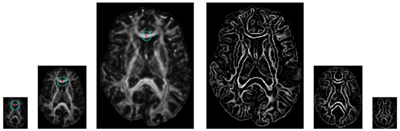
Computation of multiscale features. Instead of changing neighborhood size, the image is progressively downsampled and multiscale features are computed using a fixed neighborhood radius as indicated by the circle. This approach cuts down on the computation time. The first three images on the left show the coarse, middle and fine resolution images, respectively. The next three images show the edges detected in different resolutions.
Figure 3.
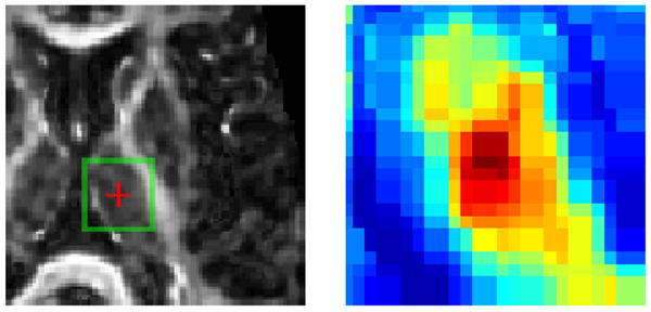
Distinctiveness of attribute vector. The similarity map in the green box is magnified for a closer inspection. Dark red indicates high similarity and dark blue otherwise.
2.3. Regional Statistical Features
For each point in the diffusion tensor image, multi-scale regional tensor distribution information can be extracted from its multi-scale neighborhoods. Specifically, for a given tensor D(x), we can extract the regional tensor distribution information from its neighborhood {D(t)|t ∈  (x)}, where
(x) is the set of coordinates of voxels in the neighborhood of x. By varying the size of neighborhood
(x) or scaling the image, we can obtain a rich set of multi-scale regional tensor distribution information, which can be used to extract tensor information at different scales and hence drive the registration hierarchically. For effective estimation of tensor distribution information, we first use logarithm to transform the original tensor to its log-space counterpart, i.e., log(D(x)), and then utilize some conventional techniques to estimate the tensor distribution information. In TIMER, we have used two commonly used statistical measures — mean and variance.
(x)}, where
(x) is the set of coordinates of voxels in the neighborhood of x. By varying the size of neighborhood
(x) or scaling the image, we can obtain a rich set of multi-scale regional tensor distribution information, which can be used to extract tensor information at different scales and hence drive the registration hierarchically. For effective estimation of tensor distribution information, we first use logarithm to transform the original tensor to its log-space counterpart, i.e., log(D(x)), and then utilize some conventional techniques to estimate the tensor distribution information. In TIMER, we have used two commonly used statistical measures — mean and variance.
But it is not necessary to stop at the means and variances. From these means and variances, we can always further derive some other features. For example, we can first utilize the mean to measure the distribution of tensors at neighborhoods of multiple scales in the log-space. A matrix exponential operation can then be performed to transform the mean M(x) back to the original tensor space, obtaining M(x), and from this tensor we can compute a series of geometric features, which can include FA, ADC, and also prolateness, oblateness, and sphericity measures as suggested in (Westin et al., 1997, 2002).
2.3.1. Regional Mean
Utilizing Log-Euclidean metrics, we can define the regional mean in a neighborhood
(x) of voxel x as:
| (3) |
where |
(x)| is the cardinality of set
(x). From the above mean, we can compute the principal diffusivities, i.e., the eigenvalues, as:
| (4) |
where represents the k-th largest eigenvalue of matrix M(x).
2.3.2. Regional Variance
Similarly, we can define the regional variance as:
| (5) |
and the principal varibilities as:
| (6) |
We scale the eigenvalues above according to the equation below to yield their mean normalized values:
| (7) |
We have used M2 instead of M to match the dynamic range of V. Note that tensor mean and variance by themselves are not orientation invariant since, as tensors, they retain orientation information. But by taking only their eigenvalues, we are effectively only keeping orientation invariant information for correspondence matching.
2.4. Boundary Features
Edge information extracted from tissue boundaries is crucial for facilitating tensor image registration especially when boundary accuracy is concerned. In TIMER, edge information from both tensors and FA map are incorporated.
2.4.1. Edge Detection on Tensors
To better extract tissue boundaries, we propose to extend Canny edge detector to cater for diffusion tensor images. Canny edge detector (Canny, 1986) is regarded as one of the best edge detectors developed in the field. It can be used to extract maximal image gradient boundaries, and is robust to noise due to the employment of Gaussian filter to smooth out noise prior to edge detection. For fast edge detection, 3D Gaussian-based image filtering is implemented using three subsequent steps of one-dimensional (1D) Gaussian filtering along the anterior-posterior, superior-inferior and left-right directions, which is then followed by gradient maps computation. Using these steps, edge detection can be accomplished rapidly and robustly. Note that in TIMER, direct tensor edge detection is performed in the logarithmic space. Log-Euclidean metrics (Arsigny et al., 2006) make this especially convenient since the operations involved are as simple as that in the classical Euclidean framework, with addition/subtraction and scaling operations properly defined. Tensor convolution with function g(x) is defined as:
| (8) |
With tensor convolution defined, operations such as Gaussian filtering and edge detection can be performed directly on the tensors. For each voxel in the volume, a gradient HTensor(x) can be computed, and from which, after non-maximum suppression, a final edge magnitude HTensor(x) can be obtained.
2.4.2. Edge Detection on FA Map
Fractional anisotropy is an important measure of the degree of anisotropy. By performing edge detection on the FA map, one can detect edges formed by highly anisotropic constituents of the brain against those which are less anisotropic. In TIMER, the edge information furnished by the FA map delineates the white matter. More details on how FA can be computed are shown in Section 2.5.1. Edges from tensors and edges from FA map are complementary to each other and, by using both, potentially all major kinds of tissue boundaries, that is, those formed between white matter (WM), gray matter (GM) and cerebro-spinal fluid (CSF), can be detected and aligned in the registration. We denote the edge magnitude returned by the FA map at point x as HFA(x).
2.5. Tensor Geometric Features
Tensor D can be decomposed into the form:
| (9) |
where λ1 ≥ λ2 ≥ λ3 and êi is the normalized eigenvector corresponding to λi. Geometrically, diffusion tensor D can be represented by an ellipsoid with three axes oriented in the direction of its eigenvectors and the semi-axis length proportional to the square root of its eigenvalues. Three different ellipsoidal shapes give rise to three geometrical structures for the diffusion tensors: prolate (linear) structure, in which diffusion is mainly in the direction corresponding to ê1; oblate (planar) structure, in which diffusion is restricted to a plane spanned by ê1 and ê2; and spherical structure with isotropic diffusion. In TIMER, we have incorporated fractional anisotropy (FA) and principal diffusivities (PD) (Basser and Pierpaoli, 1996) as part of the attribute vector to capture the tensor geometric properties, giving us microstructural information of the brain.
2.5.1. Fractional Anisotropy (FA)
Fractional Anisotropy (FA) (Basser and Pierpaoli, 1996) is defined as:
| (10) |
where is the mean diffusivity of D(x), defined as: trace(D(x))/3. FA measures the fraction of the anisotropic portion of tensor D(x). For an isotropic medium, FA = 0; for a fully anisotropic medium, FA is 1. Its value is characteristically high for a voxel containing white matter.
2.5.2. Principal Diffusivities (PDs)
Principal Diffusivities (PDs) are simply the eigenvalues of D(x):
| (11) |
They are measures of diffusivities in the principal directions. Some regions of the brain, such as the ventricles, contain mostly CSF and microstructural barriers to water mobility are sparse in these regions, although a few membranes may be present, and as a results PDs typically have high values. Owing to the inherently anisotropic nature of WM, one is able to roughly separate WM and non-WM tissues utilizing the FA map. By the same token, PD values of CSF are much larger than those of other tissues, so CSF and non-CSF tissues can be roughly separated.
2.6. Driving Voxels
Brain medical images are inherently high dimensional and computations involved in the image registration can be prohibitive. In order to overcome this, a small subset of voxels with distinctive attributive vectors, called driving voxels (Shen and Davatzikos, 2002), are selected initially to drive the registration, obtaining a coarse estimation of the registration. More driving voxels are included as the registration progresses to participate in refining the registration. TIMER selects, as driving voxels, a combination of voxels with the highest tensor edge magnitudes, FA map edge magnitudes and FA values, since these voxels represent important anatomical structures and are typically relatively easy to find in images with sufficient contrast. The driving voxels for different stages of registration are shown in Fig. 4.
Figure 4.
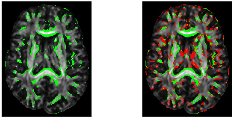
Driving voxels superimposed on the FA image. Shown on the left are the initial driving voxels and on the right the additional driving voxels, in red, when the registration progresses.
2.7. Summary of TIMER
A flowchart summarizing the working mechanism of TIMER is shown in Fig. 5. A more detailed description is provided in the following.
Figure 5.

A flowchart summarizing the main components of TIMER. The numbers in the circles refer to the corresponding text in Section 2.7.
Histogram Matching and Affine Registration: Transform the subject DT image to the template space using global affine transformation parameters which are computed based on the FA maps. Reorient the tensors (Xu et al., 2003) of the transformed subject image.
Downsampling: Downsample the DT images to an appropriate scale. Deformation field determined in this scale will be used to drive the deformation in a subsequent higher scale.
Compute Attribute Vectors: Compute an attribute vector for each voxel in the template and subject DT images, consisting of tensor edge magnitude, FA map edge magnitude, FA value, principal diffusivities, tensor mean principal diffusivities, and also principal variabilities.
Select Driving Voxels: Determine a set of driving voxels based on tensor edge magnitudes, FA map edge magnitudes, and also FA values.
Locate Correspondence: For each template driving voxel, search in its neighborhood for all subject voxels with similar attibure vectors, which is determined by a threshold which decreases with time. Tentatively deform the subvolume centered at the current template driving voxel, weighted by a Gaussian kernel, to every similar voxel found in the subject and obtain an overall degree of similarity for the deformed subvolume. This template subvolume will be deformed to the subject voxel with the largest degree of similarity, provided that the degree of similarity is over a certain predefined threshold. Note that the principle of consistent transformation (Christensen, 1999; Shen and Davatzikos, 2002) is observed in this process. For each subject driving voxel, search its neighborhood for a template driving voxel with the most similar attribute vector. If this similarity is above a threshold, which decreases with time, then the subvolume will also be deformed in the direction of the subject. If deformation field from the previous scale exists, load the deformation field for the guidance of the current cycle of correspondence matching.
Regularize Deformation Field: Refine deformation field utilizing smoothness contraints (Shen and Davatzikos, 2002).
Upsample Deformation Field: Upsample the obtained deformation field and utilize it to guide the correspondence matching of the subsequent higher scale.
Morph Subject DT Image & Reorient Tensors: If all the scales have been considered, morph the subject DT image to the template space according to the determined deformation field.
The HAMMER (Shen and Davatzikos, 2002) algorithm should be refered to if more information on step 4 to step 8 is needed.
2.8. Evaluation of TIMER
A number of experiments were performed to evaluate the accuracy of TIMER. We started off by computing a group-averaged image, which could essentially give us a visual indication of the accuracy of TIMER. This was done by first registering the diffusion tensor images of different subjects onto a randomly chosen template and then computing the average image of all the registered images. A sharp average image indicates good registration accuracy. To further evaluate the accuracy of TIMER, we simulated a set of deformation fields, which were used as ground truths. Based on these deformation fields, the respective simulated brain images could be constructed, and after registering them back onto the template, we could compare the deformation fields estimated by TIMER with the ground truths and quantify the registration accuracy. To gauge the effectiveness of TIMER in aligning the brain microstructures, especially those in the white matter, a fiber tracking was performed, where the consistency of the fiber bundles in the simulated brains were compared with those in the template. We also performed an experiment using simulated brain atrophy to gauge whether an arophic region remains detectable after registration. Lastly, we performed a noise sensitivity study to evaluate how well TIMER can perform under different signal-to-noise ratios (SNRs). Whenever appropriate, results obtained using DTI registration algorithms proposed by Yang et al. (Yang et al., 2008a) and Zhang et al. (Zhang et al., 2006) will be included for comparison, and they will be referred to as YANG and ZHANG1 respectively in rest of the paper.
2.8.1. Real Subjects
A direct and intuitive way of gauging the accuracy of a registration algorithm is by inspecting the sharpness of an average image obtained from a set of aligned images. Inaccurate registration often results in the improper alignment of wrong anatomical structures, and when averaged, will result in fuzziness of the final image. To evaluate TIMER, we took a similar approach where one subject was selected as the template for the dataset, and the other 21 subjects were then registered onto this template to form the average image. For easier inspection, a standard deviation map can be generated. The standard deviation value at each voxel location gives us information on the extent of tensor deviation of the aligned images from the average image. For this purpose, we employed the tensor normalized standard deviation, defined by Jones et al. (Jones et al., 2002) as:
| (12) |
where ||·||F is the Frobenius norm, and D̄ the tensor mean, computed by element-wise averaging, of the same voxel location from a set of N diffusion tensor images, and Dk is the tensor from the kth image. Another useful metric for alignment evaluation is the normalized scalar product applied to the FA map of each individual registered image with respective to the template. Given the FA maps of the template, I(x), and the subject, J(x), the normalized scalar is defined as:
| (13) |
where u(x) is the subject-to-template deformation field and  denotes the brain image volume.
2.8.2. Simulated Subjects
To further evaluate the accuracy of TIMER, we generated a set of simulated deformation fields using the statistical model of deformation (SMD) proposed by Xue et al. (Xue et al., 2006). In this approach, Wavelet-Packet Transform (WPT) of the training deformations and their Jacobians, in conjunction with a Markov random field (MRF) spatial regularization, are used to capture both coarse and fine characteristics of the training deformations in a statistical fashion. Simulated deformations can then be generated by randomly sampling the resultant statistical distribution (Xue et al., 2006). One human brain was utilized as the template and the 20 simulated deformation fields, which also served as the ground truths, were applied to the template, resulting in 20 simulated human brains. These 20 simulated brains were then registered back onto the template using TIMER and the deformation fields estimated by the registration were compared with the ground truths. The accuracy of the estimated deformation fields were evaluated by the average difference m̄d and the standard deviation (SD) σd of the two deformation fields, i.e. (Yang et al., 2008b):
| (14) |
and
| (15) |
where ||·|| is the Euclidean distance, || the number of voxels in the brain image volume , and ug(x), ue(x) the template-to-subject deformation vectors at location x of the ground truth deformation field and the estimated deformation field, respectively.
2.8.3. Fiber Tracking
Local diffusion patterns characterized by the restricted motion of cellular fluid within brain white matter gives an estimation of the orientation of the underlying fibers. The potential of DTI, capitalizing on this fact, to reveal white matter integrity, disruption and pathology makes it the preferred modality for studying white matter diseases. Accurate DTI registration is essential to establish intersubject homology for further statistical inference. Using a tractography method known as Fiber Assignment by Continuous Tracking (FACT) (Mori et al., 1999; Xue et al., 1999), fiber bundles passing through some regions of interest (ROIs) were tracked, extracted, and compared for quantifying how well TIMER performs in these specific ROIs. Fiber tracking was performed in DTI Studio (Jiang et al., 2006), with the FA start tracking threshold set to 0.25 and the FA stopping threshold set to 0.2. A turning angle of 70° stops the tracking. The same fiber tracking procedure was performed on the TIMER registered simulated brains, their group-averaged mean and also the template itself. By comparing the similarity of the fiber tract bundles, we could gauge the effectiveness of TIMER in registering the images. The distance of two fiber bundles was then measured in a way similar to that used in (Zhang et al., 2006). The distance measure is defined as:
| (16) |
where d(·, ·) is a pairwise distance between two fibers in bundles ℱ and  , which in our case is the Euclidean distance. When two fiber bundles are perfectly aligned, the value returned is zero. This measure, similar to what is referred to as the mean of the closest distances, approximately establish anatomic correspondences between points along fibers from different subjects.
2.8.4. Atrophy Detection
We simulated hypothetical abnormality, affecting the tensors in a specific brain region, and gauge the detectability of the abnormal region after registration. We simulated atrophic brains based on the healthy brains that we had created in Section 2.8.2 and, after registering them onto the template, we wanted to determine whether the atrophic region was still detectable, gauged using t-test. We first defined a region of interest on a main fiber pathway on the template image, and we could then map this region of interest onto the simulated brains based on their respective simulated deformation fields. These regions on the simulated brains were then perturbed with a hypothetical atrophy, which effectively made the tensors more isotropic (rounder and less elongated ellipsoids) and hence had smaller FA values. Let D be the tensor with eigenvalues λ1 ≥ λ2 ≥ λ3 and eigenvectors v1, v2 and v3. For a degradation percentage η, we simulated the atrophy as follows:
Step 1: Let λ = max(λ1, λ2, λ3)
Step 2: Set , ∀i
-
Step 3: Set
Step 4: Randomly peturb the tensor angle with an orthogonal rotation matrix2 R by a maximum value of θmax:
| (17) |
Directions of anisotropic tensors are perturbed more than the isotropic ones.
Obviously, at η = 1.0 the resultant tensor D′ will be perfectly isotropic, the FA value of which is 0; at η = 0.0, the original eigenvalues are retained. By performing paired t-tests on the FA maps of the healthy brains and those with simulated atrophy, we could gauge how well the detectability of the atrophic regions was retainted after registration with TIMER. Detected regions with a false discovery rate (FDR) of 0.05 was retained and deemed significant. The Dice ratio (Dice, 1945) was computed for the detected region with respect to the ground truth atrophic region, a higher value of which indicated a more accurate match of the detected region and hence less false positives and/or false negatives.
2.8.5. Noise Sensitivity
Due to the signal-attenuation nature of diffusion encoding and the inadvertent T2 relaxation resulting from the long TE necessary to accommodate the sensitization gradient pulses, the signal-to-noise ratio (SNR) of DTI is inherently low (Chen and Hsu, 2005). The simplest means of improving the effective SNR is by acquiring more signals for averaging, using more diffusion sensitization directions, encoding levels, or a combination of these. Regardless of the strategy, the scan time is necessarily and proportionally lengthened. For these reasons, it is important that algorithms developed for diffusion tensor images are robust to noise and are able to perform satisfactorily in low SNR conditions as such. A simple SNR sensitivity evaluation of a registration algorithm can be carried out by generating some noisy images, register them onto the template, and compare their registration accuracy with respect to their noise free counterparts. In order to ensure that, after adding noise, the diffusion tensors remain symmetric positive definite (SPD), we first decompose the diffusion tensors using Cholesky decomposition (Bergmann et al., 2007):
| (18) |
where L is a lower triangular matrix with strictly positive diagonal entires, and LT denotes the tranpose of L. Adding noise on the elements of L, forming L̃, we can obtain a SPD noisy diffusion tensor D̃ = L̃L̃T.
3. Results
3.1. Results: Real Subjects
The average images generated by registering 21 subjects onto the template are shown in Fig. 6. It can be observed that for FA map based affine registration, the average image, shown in Fig. 6(b), is fuzzy especially in areas near the cortical surface. In comparison, TIMER yields an average image, shown in Fig. 6(c), which shows much improved sharpness. By superimposing the edges of the FA map of the average image on the FA map of the template, as shown in Fig. 7, we can see that the white matter edges of the images are properly aligned, indicative of good registration accuracy. For convenient visual inspection, the normalized standard deviation maps are shown in Fig. 8. The images yielded by TIMER are generally darker in both cortical and subcortical regions, implying less registration variability and closer resemblance of tensors at corresponding locations of different subjects. The scalar product values, averaged over all 21 registered images, yielded by TIMER, YANG, ZHANG and affine registration are 0.9126, 0.9094, 0.8894, and 0.8293, respectively. The relative high value given by TIMER once again validate its performance superiority compared to other methods.
Figure 6.

Group-averaged images resulting from the registration of the 21 subjects. The FA weighted first principal directions are shown in their color coded representations: green for the anterior-posterior direction, blue for the superior-inferior direction, and red for the left-right direction. The tensors in the yellow boxes are shown in their FA weighted ellipsoidal representations in the bottom panels.
Figure 7.
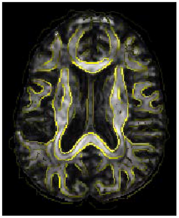
White matter edges generated from the FA map of the average tensor image is overlaid on the template. The proper alignment of the edges is indicative of good registration accuracy.
Figure 8.

Normalized standard deviation. The images in the top row are slices of the normalized standard deviation map generated from the TIMER registered images; the images in the bottom row are those from affine registration.
3.2. Results: Simulated Subjects
We generated two sets (Set I & Set II) of simulated deformation fields. Set I consisted of 20 deformation fields, which were more regular and generally had smaller displacement magnitudes, whereas Set II contained the same number of deformation fields, but were more complex and had larger magnitudes, generated using a larger variance in SMD (Xue et al., 2006). Fig. 9(a) shows some typical deformation fields and images from Set I and Set II. The deformation estimation errors for Set I are shown in Fig. 9(b). The average error for the 20 simulated brains is 0.83mm, which indicates that TIMER is accurate to a subvoxel level. A summary of the results for the whole brain and also the cortical region in comparison with YANG and ZHANG is provided in Table 1. For Set I, the accuracy yielded by TIMER is closely followed by that of ZHANG and is better than YANG by a larger margin. But for Set II, the improvement brought by TIMER is clearly quite significant. For all cases, TIMER is also more consistent as indicated by the smaller standard deviation values. Similar conclusion can be drawn from the results of the cortical region.
Figure 9.

(a) Difference between Set I and Set II. Middle: Template. Middle left and left: an image in Set I with its template-to-subject deformation field; Middle right and right: an image in Set II with its deformation field. The deformation fields of images in Set II are characteristically more irregular and larger in magnitudes compared with the more conservative deformation fields of Set I. In the different panels, markers with the same color are placed at the same location to facilitate comparison. (b) Deformation field errors of TIMER compared to the ground truths. The average deformation field error of the 20 simulated brains is 0.83mm with a standard deviation of 0.48mm.
Table 1.
Averages and Standard Deviations of Deformation Estimation Errors (mm).
| Whole Brain | Cortical Region | ||||||
|---|---|---|---|---|---|---|---|
| TIMER | YANG | ZHANG | TIMER | YANG | ZHANG | ||
| Set I | Mean | 0.83 | 1.36 | 0.84 | 0.86 | 1.44 | 0.92 |
| Std. Deviation | 0.48 | 0.82 | 0.76 | 0.47 | 0.82 | 0.81 | |
|
| |||||||
| Set II | Mean | 1.11 | 1.87 | 1.44 | 1.18 | 2.03 | 1.68 |
| Std. Deviation | 0.82 | 1.48 | 1.75 | 0.88 | 1.59 | 1.96 | |
3.3. Results: Fiber Tracking
We present here two sets of results. For Set I, two ROIs were selected so that two fiber bundles, one residing in the genu and the other in the splenium of the corpus callosum (CC), could be extracted for comparison. For Set II, we evaluated TIMER in a more difficult situation where a fiber bundle near the cortical surface was considered. Registration of near cortical surface regions is often the Achilles’ heel of many registration algorithms. All the fiber bundles are shown in Fig 10(a). Detailed results for TIMER for the genu and splenium fiber bundles are shown in Fig. 10(b). A summary of the results of all fiber bundles, with those of YANG and ZHANG included, is shown in Table 2. Due to the inherent nature of fiber tracking, accurate registration of the fiber bundles are not only determined by the correct estimation of the deformation field, as was examined in the previous experiment, but also by the correct reorientation of tensors. TIMER incorporates a tensor reorientation scheme which attempts to estimate the underlying fiber orientation by considering an appropriate small neighorbood around each voxel (Xu et al., 2003), and is hence less vulnerable to noise. This is attested by the results yielded by TIMER in comparison with YANG and ZHANG, where fiber bundles extracted with TIMER are consistently closer to the ground truths.
Figure 10.

(a) Template fiber bundles used as the ground truths for evaluation. The fiber bundles shown in yellow and green reside in the genu and the splenium of the corpus callosum, respectively. In red is a fiber bundle near the cortical surface. Fibers shown here are all from the template image. (b) Distances of fiber bundles extracted from the simulated brains (Set I) compared to the template. The yellow and green bars show the results for the genu and the splenium fiber bundles, respectively. Subject 21 is the group-averaged mean. The average errors for the genu and the splenium fiber bundles are 0.62mm and 0.77mm, respectively. Results from Set II (red fibers in (a)) are not shown in this graph as their higher fiber distance values would overwhelm those yielded by Set I. Moreover, Set I and Set II consist of different simulated subjects.
Table 2.
Average Fiber Distances (mm)
| TIMER | YANG | ZHANG | ||
|---|---|---|---|---|
| Set I | Genu | 0.62 | 0.78 | 0.67 |
| Splenium | 0.77 | 0.82 | 1.00 | |
|
| ||||
| Set II | Cortical | 1.25 | 1.49 | 1.91 |
3.4. Results: Atrophy Detection
We used η = 0.05, 0.10, 0.40 and θmax = 10° to generate 3 × 20 simulated brains with atrophy using Set I. Fig. 11 shows the region with simulated atrophy and their ellipsoidal representation images before and after the introduction of atrophy. The atrophy detection results are shown in Table 3. It is worth noting that in order to maintain the detection specificity of the atrophic region, i.e. high Dice ratio, the registration algorithm used, while maintaining the detectability of the atrophic region, should not be overtly sensitive to the changes brought about by the abnormalities. If not so, the registration of the surrounding non-atrophic regions will be affected and will hence result in low specificity due to false positives. This problem is mitigated by the multiscale mechanism in TIMER, the coarse scale features of which effectively help avoid the aforementioned pitfall by considering a regional neighborhood which is often larger than the atrophic region. TIMER therefore has a less tendency of being influenced by the atrophic region itself and of propagating the abnormalities to other non-atrophic regions in the course of registration. And it is thus not suprising here that the Dice ratios yielded by TIMER are consistently higher. On average, TIMER yields a 0.2 unit improvement over YANG and 0.5 unit over ZHANG. The affine registered images fail to capture the subtlety of the atrophy, rendering the atrophic region undetectable.
Figure 11.

Simulated atrophy. The content in the green box (a) is enlarged with its ellipsoidal representation images before and after the introduction of atrophy shown in (b) and (c), respectively. The tensors are fatter when atrophic. The changes in directions can be noticed from the change of colors.
Table 3.
Dice Ratios of Detected Regions Relative to the Ground Truth Atrophic Region
| η | TIMER | YANG | ZHANG | AFFINE |
|---|---|---|---|---|
| 0.05 | 0.81 | 0.61 | 0.41 | 0.00 |
| 0.10 | 0.89 | 0.75 | 0.35 | 0.00 |
| 0.40 | 0.83 | 0.59 | 0.25 | 0.00 |
3.5. Results: Noise Sensitivity
We tested the SNR sensitivity of TIMER by measuring the decrease of registration accuracy (via measuring the deformation estimation error), using 10 randomly selected subjects from Set I and Set II. Additive Gaussian noise of standard deviations, σ = 0.005, 0.01, 0.02, is used. Some sample images are shown in Fig. 12. The results indicate that TIMER is robust to noise, as validated by the low percentages of accuracy decreases — −0.0076%, 0.60%, and 1.33%, respectively.
Figure 12.

Noise degraded images. The original image, on the top left, followed by images with increasing degrees of noise (σ = 0.005, 0.01, 0.02).
4. Discussion
In medical imaging, it is important to build deformable anatomical models that take into account the underlying anatomy, and not simply the similarity of image intensities. To this end, a multiscale attribute vector is attached to each voxel, reflecting its underlying anatomical structure in a local scale, and also its relationship to more distant voxels in a more global scale. A rich enough attribute vector can potentially differentiate different parts of the anatomy that would otherwise look similar. Relative high variability of brain structures makes certain features, especially those capturing detailed features, vary dramatically accross individual brains, thus confounding the image matching procedure. It is hence desirable that features used for image matching be robust to structural variations across individuals. Since orientation variation can be part of the confounding factor in the matching process, features used preferably should also be invariant to rotations. A number of such features can be collected to form attribute vectors for correspondence matching in registration. Attribute vectors are a critical part of TIMER. An attribute vector is defined for each voxel in a volumetric image, and it reflects the underlying structure at multiple scales. Each attribute vector in TIMER characterizes the voxel in terms of its regional tensor mean, regional tensor variance, diffusivity, tensor edge magnitude, FA map edge magnitude and FA value. As can be attested by the experiments, attribute vector as such is sufficiently rich to guide the registration. The attribute vectors are used to morph the subject onto the template using a deformable scheme similar to that of HAMMER (Shen and Davatzikos, 2002). After registration, tensor at each voxel is reoriented using the Procrustean estimation approach proposed in (Xu et al., 2003). Registration of images with dimension 256 × 256 × 70 takes approximately 90 minutes on a 2.66GHz Linux machine. Images with smaller dimension, e.g., 128 × 128 × 46, take around 30 minutes.
4.1. Tract-Based Spatial Statistics (TBSS)
In their TBSS paper (Smith et al., 2006), Smith et al. argue that, to sufficiently align images for subsequent statistical analysis, a non-linear alignment with intermediate degrees of freedom (DoF) has to be used. The main concern is that while low-DoF barely guarantees the proper alignment of structural details, high-DoF jeopardizes structural topology, causing biologically incorrect results. The formulation of TIMER ascertain that the pitfalls at both DoF extremes can be avoided. While the correspondence matching mechanism of TIMER is inherently high-DoF, it is regularized by a smoothness contraint which ensures proper topological preservation. In fact, it is perceivable that TIMER can easily be incorporated in the framework of TBSS for effective analysis of tract statistics. TIMER can be employed to non-linearly register the images onto a selected template, form the mean diffusion tensor image and its FA map, and generate the tract skeleton. After projecting the individual subjects’ FA values onto the skeleton, the spatially aligned FA values can be extracted for voxelwise cross-subject statistical analysis.
4.2. Brain Tumors
Existing brain image registration algorithms are generally unable to account for topological differences between a brain with tumor and a normal brain. The effects of edema, tissue death and resorption, tissue infiltration, tumor mass-effect, cause servere deformation atypical of natural inter-subject variability to which these algorithms are tuned. As a future work, TIMER can be tuned to account for abnormality as such. One possible approach is by adopting the method proposed by Mohamed et al. (Mohamed et al., 2006), where a biomechanical three-dimensional model is employed to simulate the deformation caused by the tumor bulk and the peri-tumor edema. The estimation of the deformation field is decomposed into two components, one representing inter-individual brain shape differences, and the other representing tumor-induced deformation. For facilitating registration, a simulation of tumor mass-effect is performed on the template image to generate an image that is similar to the image of the brain with tumor.
4.3. Concluding Remarks
In conclusion, Tensor Image Morphing for Elastic Registration or TIMER is proposed as a relatively accurate diffusion tensor registration algorithm in this paper. The main novelty of TIMER lies in its direct extraction of regional and edge information from the tensors to guide the registration in a hierarchical fashion. Using these features to drive the registration, it is found that subvoxel accuracies can be achieved with an average deformation field estimation accuracy of 0.83mm. The directional structure of the tensors are also retained accurately, as can be attested by the fiber tracking experiment, which returns an average accuracy of 0.62mm, 0.77mm and 1.32mm for the genu, splenium and near cortical fiber bundles, respectively. Pathological cues such as atrophy detectability is also retained after the registration, which is indicated by the typically high Dice ratios. Table 4 provides a summary of improvements brought about by TIMER in terms of p values obtained from a series of paired t-tests3. Although TIMER performs reasonably well in all experiments performed, we feel that there is still room for improvement. One possible direction is to employ an example based learning method to learn separate sets of appropriate features for registration guidance of different brain regions. Research in this direction can be conducted with the hope of a more refined DTI registration algorithm.
Table 4.
Improvement of TIMER Over YANG and ZHANG in Terms of Paired t-Test p-Values.
| YANG | ZHANG | |
|---|---|---|
| Real Subjects* (Section 3.1) | p = 4.92 × 10⁻⁴ | p = 3.54 × 10⁻¹⁴ |
| Simulated Subjects** (Section 3.2) | p = 8.69 × 10⁻²⁵ | p = 2.98 × 10⁻⁵ |
| Fiber Tracking*** (Section 3.3) | p = 4.57 × 10⁻⁶ | p = 2.68 × 10⁻⁸ |
All scalar product values,
All estimated deformation field errors,
All fiber bundle distances
Acknowledgments
The authors would like to express their gratitude to Gary Zhang of Penn Image Computing and Science Lab (PISCL) for helping us understand his algorithm better and for his graciousness in optimizing the code for the comparisons conducted in this paper.
Appendix: Generation of 3D Random Rotation Matrix
A rotation matrix to rotate about any arbitrary axis can be constructed using:
| (19) |
where
| (20) |
and (x, y, z) is a unit vector on the axis of rotation. For a tensor D with eigenvalues λ1 ≥ λ2 ≥ λ3 and eigenvalues v1, v2 and v3 we can find a random axis of rotation in the plane defined by v2 and v3, i.e.:
| (21) |
where a and b are random arbitrary numbers. We can then rotate the principal direction as defined by v1 using (19) by a random angle, θ, between 0 and θmax.
Footnotes
The version used in our experiments is an extension of (Zhang et al., 2006), which can handle relatively larger deformations as mentioned in (Zhang et al., 2007).
See Appendix for explanation on how a random rotation matrix can be generated.
The values used in the paired t-tests are listed as follows: Real Subjects (Section 3.1), all values from the scalar products; Simulated Subjects (Section 3.2), all estimated deformation field errors; and Fiber Tracking (Section 3.3), all fiber bundle distances.
Publisher's Disclaimer: This is a PDF file of an unedited manuscript that has been accepted for publication. As a service to our customers we are providing this early version of the manuscript. The manuscript will undergo copyediting, typesetting, and review of the resulting proof before it is published in its final citable form. Please note that during the production process errors may be discovered which could affect the content, and all legal disclaimers that apply to the journal pertain.
References
- Alexander DC. An Introduction to Computational Diffusion MRI: the Diffusion Tensor and Beyond. Springer Berlin Heidelberg, Ch; 2006. Visualization and Processing of Tensor Fields; pp. 83–106. [Google Scholar]
- Arsigny V, Fillard P, Pennec X, Ayache N. Log-Euclidean metrics for fast and simple calculus on diffusion tensors. Magnetic Resonance in Medicine. 2006;56 (2):411–421. doi: 10.1002/mrm.20965. [DOI] [PubMed] [Google Scholar]
- Basser PJ, Pierpaoli C. Microstructural and physiological features of tissues elucidated by quantitative-diffusion-tensor MRI. Journal of Magnetic Resonance Series B. 1996;111 (3):209–219. doi: 10.1006/jmrb.1996.0086. [DOI] [PubMed] [Google Scholar]
- Bergmann Ø, Christiansen O, Lie J, Lundervold A. Shape-adaptive dct for denoising of 3d scalar and tensor valued images. Journal of Digital Imaging. 2007 December; doi: 10.1007/s10278-007-9088-6. [DOI] [PMC free article] [PubMed] [Google Scholar]
- Canny J. A computational approach to edge detection. IEEE Transactions on Pattern Analysis and Machine Intelligence. 1986;8:679–714. [PubMed] [Google Scholar]
- Chen B, Hsu EW. Noise removal in magnetic resonance diffusion tensor imaging. Magnetic Resonance in Medicine. 2005;54:393–407. doi: 10.1002/mrm.20582. [DOI] [PubMed] [Google Scholar]
- Christensen GE. Information Processing in Medical Imaging. 1999. Consistent linear-elastic transformations for image matching; pp. 224–237. [Google Scholar]
- Dice LR. Measures of the amount of ecologic association between species. Ecology. 1945;26:297–302. [Google Scholar]
- Huang H, Zhang J, Wakana S, Zhang W, Ren T, Richards L, Yarowsky P, Donohue P, Graham E, van Zijl PCM, Mori S. White and gray matter development in human fetal, newborn and pediatric brains. NeuroImage. 2006;33 (1):27–38. doi: 10.1016/j.neuroimage.2006.06.009. [DOI] [PubMed] [Google Scholar]
- Jiang H, van Zijl PCM, Kim J, Pearlson GD, Mori S. DtiStudio: resource program for diffusion tensor computation and fiber bundle tracking. Computer Methods and Programs in Biomedicine. 2006 February;81 (2):106–116. doi: 10.1016/j.cmpb.2005.08.004. [DOI] [PubMed] [Google Scholar]
- Jones DK, Griffin LD, Alexander DC, Catani M, Horsfield MA, Howard R, Williams SCR. Spatial normalization and averaging of diffusion tensor MRI data sets. Neuroimage. 2002;17:592–617. [PubMed] [Google Scholar]
- Lazebnik S, Schmid C, Ponce J. A sparse texture representation using local affine regions. IEEE Transactions on Pattern Analysis and Machine Intelligence. 2005;27:1265–1278. doi: 10.1109/TPAMI.2005.151. [DOI] [PubMed] [Google Scholar]
- Lee A, Lepore N, Barysheva M, Chou Y, Brun C, Madsen SKLM, de Zubicaray G, Meredith M, Wright M, Toga A, Thompson P. Comparison of fractional and geodesic anisotropy in diffusion tensor images of 90 monozygotic and dizygotic twins. ISBI’2008. 2008 May; doi: 10.1109/ISBI.2008.4541153. [DOI] [PMC free article] [PubMed] [Google Scholar]
- Liu T, Li H, Wong K, Tarokh A, Guo L, Wong ST. Brain tissue segmentation based on DTI data. NeuroImage. 2007;38 (1):114–123. doi: 10.1016/j.neuroimage.2007.07.002. [DOI] [PMC free article] [PubMed] [Google Scholar]
- Lowe D. Distinctive image features form scale-invariant key-points. International Journal of Computer Vision. 2004;2:91–110. [Google Scholar]
- Mohamed A, Zacharaki EI, Shen D, Davatzikos C. Deformable registration of brain tumor images via a statistical model of tumor-induced deformation. Medical Image Analysis. 2006;10:752 – 763. doi: 10.1016/j.media.2006.06.005. [DOI] [PubMed] [Google Scholar]
- Mori S, Crain BJ, Chacko VP, van Zijl PCM. Three-dimensional tracking of axonal projections in the brain by magnetic resonance imaging. Annals of Neurology. 1999;47 (2):265–269. doi: 10.1002/1531-8249(199902)45:2<265::aid-ana21>3.0.co;2-3. [DOI] [PubMed] [Google Scholar]
- Mori S, Itoh R, Zhang J, Kaufmann WE, Zijl PCMV, Solaiyappan M, Yarowsky P. Diffusion tensor imaging of the developing mouse brain. Magnetic Resonance in Medicine. 2001;46 (1):18–23. doi: 10.1002/mrm.1155. [DOI] [PubMed] [Google Scholar]
- Mukundan R, Ramakrishnan K. Moment functions in image analysis – Theory and Applications. World Scientific Publishing; Singapore: 1998. [Google Scholar]
- Pierpaoli C, Jezzard P, Basser JP, Barnett A, Chiro GD. Diffusion tensor MR imaging of human brain. Radiology. 1996;201 (3):637–648. doi: 10.1148/radiology.201.3.8939209. [DOI] [PubMed] [Google Scholar]
- Shen D. Image registration by local histogram matching. Pattern Recognition. 2007;40:1161–1171. [Google Scholar]
- Shen D, Davatzikos C. HAMMER: Heirarchical attribute matching mechanism for elastic registration. IEEE Transactions on Medical Imaging. 2002;21 (11):1421–1439. doi: 10.1109/TMI.2002.803111. [DOI] [PubMed] [Google Scholar]
- Smith S, Jenkinson M, Johansen-Berg H, Rueckert D, Nichols T, Mackay C, Watkins K, Ciccarelli O, Cader M, Matthews P, Behrens T. Tract-based spatial statistics: Voxelwise analysis of multi-subject diffusion data. Neuroimage. 2006;31 (4):1487 – 1505. doi: 10.1016/j.neuroimage.2006.02.024. [DOI] [PubMed] [Google Scholar]
- Westin CF, Maier SE, Mamata H, Nabavi A, Jolesz FA, Kikinis R. Processing and visualization of diffusion tensor MRI. Medical Image Analysis. 2002;6 (2):93–108. doi: 10.1016/s1361-8415(02)00053-1. [DOI] [PubMed] [Google Scholar]
- Westin C-F, Peled S, Gudbjartsson H, Kikinis R, Jolesz FA. Geometrical diffusion measures for MRI from tensor basis analysis. ISMRM ’97. 1997 April;:1742. [Google Scholar]
- Xu D, Mori S, Shen D, van Zijl PCM, Davatzikos C. Spatial normalization of diffusion tensor fields. Magnetic Resonance in Medicine. 2003 July;50 (1):175–182. doi: 10.1002/mrm.10489. [DOI] [PubMed] [Google Scholar]
- Xue R, van Zijl PCM, Crain BJ, Solaiyappan M, Mori S. In vivo three-dimensional reconstruction of rat brain axonal projections by diffusion tensor imaging. Magnetic Resonance in Medicine. 1999;42 (6):1123–1127. doi: 10.1002/(sici)1522-2594(199912)42:6<1123::aid-mrm17>3.0.co;2-h. [DOI] [PubMed] [Google Scholar]
- Xue Z, Shen D, Karacali B, Stern J, Rottenberg D, Davatzikos C. Simulating deformations of MR brain images for validation of atlas-based segmentation and registration algorithms. NeuroImage. 2006;33 (3):855–866. doi: 10.1016/j.neuroimage.2006.08.007. [DOI] [PMC free article] [PubMed] [Google Scholar]
- Yang J, Shen D, Davatzikos C, Verma R. Diffusion tensor image registration using tensor geometry and orientation features. MICCAI’08. 2008a;11(Pt 2):905–913. doi: 10.1007/978-3-540-85990-1_109. [DOI] [PubMed] [Google Scholar]
- Yang J, Shen D, Misra C, Wu X, Resnick S, Davatzikos C, Verma R. Medical Imaging 2008: Image Processing. Vol. 6914. SPIE; 2008b. Spatial normalization of diffusion tensor images based on anisotropic segmentation; p. 69140L. [Google Scholar]
- Zhang H, Avants BB, Yushkevich PA, Woo JH, Wang S, McCluskey LF, Elman LB, Melhem ER, Gee JC. High-dimensional spatial normalization of diffusion tensor images improves the detection of white matter differences: An example study using amyotrophic lateral sclerosis. IEEE Transactions on Medical Imaging. 2007 November;26 (11):1585–1597. doi: 10.1109/TMI.2007.906784. [DOI] [PubMed] [Google Scholar]
- Zhang H, Yushkevich PA, Alexander DC, Gee JC. Deformable registration of diffusion tensor MR images with explicit orientation optimization. Medical Image Analysis. 2006;10 (5):764–785. doi: 10.1016/j.media.2006.06.004. [DOI] [PubMed] [Google Scholar]