Determination of Signal-to-Noise Ratios and Spectral SNRs in Cryo-EM Low-dose Imaging of Molecules

Abstract

Attempts to develop efficient classification approaches to the problem of heterogeneity in single-particle reconstruction of macromolecules require phantom data with realistic noise models. We have estimated the signal-to-noise ratios and spectral signal-to-noise ratios for three steps in the electron microscopic image formation from data obtained experimentally. An important result is that structural noise, i.e. the irreproducible component of the object prior to image formation, is substantial, and of the same order of magnitude as the reproducible signal. Based on this result, the noise modeling for testing new classification techniques can be improved.

Introduction

Current attempts to develop smart classification methods for classification of heterogeneous data for single-particle reconstruction (Elad et al., 2007; Fu et al., 2007; Kalinowski and Herman, 2008; Scheres et al., 2007a,b; see Frank, 2006) require a scoring on what constitutes successful classification. Unfortunately, for experimental data there exists no a priori knowledge on the class membership of an individual particle. The need for a suitable model dataset has therefore been recognized (Scheres et al., 2007a,b). In this study we have set out to determine parameters for a realistic data model for a typical dataset of projections of single molecules embedded in ice and imaged at low-dose conditions. The most important parameter is the signal-to-noise ratio of noise sources at different steps of the imaging process. With a three-dimensional phantom object explicitly given, once the value of this parameter is known for each step, a set of images can be modeled by using randomly-drawn projection angles and random realizations of the noise, additionally taking into account the contrast transfer mechanism in TEM bright field.

In our work we make use of a relationship that links the signal-to-noise ratio (SNR) of an image to the cross-correlation coefficient (CCC) determined from a pair of images recorded in a repeated experiment under the same conditions (Frank and Al-Ali, 1975). This relationship has been used in a number of studies to estimate the SNR in bright-field TEM imaging (e.g., Elad et al., 2007; Fu et al., 2007). In such an experiment, the signal portions are identical while the noise portions are different realizations of the same statistical distribution.

$$\alpha =\rho /(1-\rho )$$ (1)

where α is the SNR, as usually defined as the ratio of the signal power to the noise power, and ρ is the CCC. When imaging a set of molecules with identical structure in the electron microscope, we can see noise interfering at three stages: (1) the molecule is surrounded by a matrix of ice; and often a thin carbon film is superimposed. From one molecule to the next, this “background structure” is irreproducible, and is therefore often called “structural noise.” Conceptually, we must also count as “background structure” any part of the molecule structure that is not reproducible, due to conformational variations. (2) Any image of a structure obtained in the electron microscope is subject to “shot noise”, due to the quantum nature of the electron radiation. (3) The recording and digitization event itself is subject to noise: if by photographic recording and subsequent digitization, the noise is manifested in photographic granularity and digitization noise in the microdensitometer; if by CCD camera, the noise is manifested in readout noise.

To make use of the SNR measurement via CCC, we can devise experiments for each of the three stages of the noise process, in which the imaging step “above” the noise process is duplicated. For clarity, we make use of a diagram in which the imaging process is symbolized by a communication channel with three intervening noise processes. Duplication of a partial path of this channel is indicated by a branched graph, with the branching going off at different levels. Each experiment yields two images at the end.

In the first such experiment (Fig. 1a), we compare images of two molecules that were identified, by the projection matching algorithm, as having the same orientation. These molecules can be modeled as one idealized molecule superimposed with two realizations of “structural noise”, that is, the structure of the support as well as any conformational differences characterizing the deviation of the actual molecules from the ideal. In addition, the two images differ both in the shot noise and the digitization noise since these are independently added. The CCC of this image pair is denoted ρ_struct.

Figure 1.

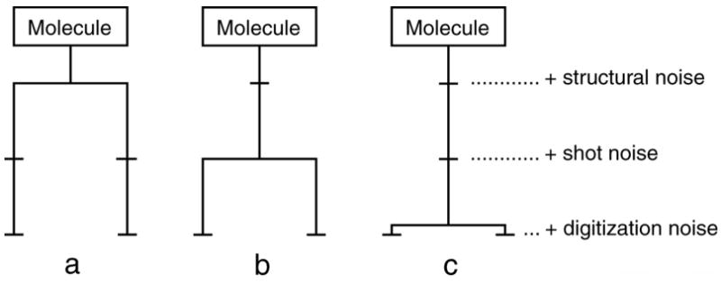
Principle of SNR measurement by double experiments, each of which results in a pair of images. a) Image pairs with the same orientation (i.e., oriented to the same reference) result from separate processing pathways with different structural noise, shot noise, and digitization noise. The cross-correlation coefficient α_struct is computed from this comparison, yielding SNR α_{comp_struct}. b) Image pairs from two exposures of the same imaging field have different shot noise and digitization noise (but same structural noise), yielding cross-correlation coefficient ρ_exp and SNR α_{comp_exp}. c) Image pairs obtained by twice scanning the same micrograph have the same structural and shot noise, but different digitization noise, yielding ρ_scan and α_{true_scan}. See text for details.

In the second experiment (Fig. 1b), we compare two images of the same molecule, taken successively in the electron microscope under identical dose conditions. In this case, a unique structure of molecule and background is subject to two different two-stage noise processes, each made up of shot noise, and digitization noise (in the case of recording on film this includes granularity of the emulsion). The CCC of this image pair, from two exposures of the same field, is denoted ρ_exp.

In the third experiment (Fig. 1c), we aim at separating shot noise and noise due to granularity from the digitization noise. This is accomplished by digitizing the same molecule image twice, and comparing the resulting digital representations, to obtain ρ_scan.

Only the third experiment gives an immediate answer through application of equation (1). In the other two cases, the noise portions from different sources are intermingled, and the SNR of each step must be obtained by considering the cascading of the noise processes, as already proposed by Frank and Al-Ali (1975) for considering the digitization noise. For a simpler system, in which two noise processes sub1 and sub2 are active,

$${\alpha }_{\mathit{sub}1}=\frac{1}{(1+1/{\alpha }_{\mathit{comp}})/(1+1/{\alpha }_{\mathit{sub}2})-1}$$ (2)

where α_sub1 is the SNR of sub-process 1, α_sub2 the SNR of sub-process 2, and α_comp is the SNR measured for the entire imaging process, being a composite of the two subprocesses. In the case of three subsystems, equation (2) simply has to be used repeatedly.

The SNRα is computed from CCC ρ for the three sub-processes: dual scan pairs for the digitization SNR (α_scan), dual exposure pairs for the SNR related to shot noise (α_exp), and pairs of images aligned to the same reference projection for structural SNR (α_struct). A further distinction is made between composite SNR composed of intermingled noise sources (α_comp), and the actual SNR (α_true) calculated by equation 2, which untangles the noise sources. Equation 1 yields α_comp in the case of shot noise and structural SNR, α_true in the case of digitization noise. Thus α_{comp_exp} is the shot noise SNR measured from dual exposure image pairs, while α_{true_exp} is the actual SNR related to shot noise computed from equation 2 by substituting α_{true_scan} for α_sub2, and α_{comp_exp} for α_comp. Similarly, α_{comp_struct} is obtained from the directly measured ρ_struct of same-reference image pairs, while α_{true_struct} is the actual structural SNR computed by substituting α_{comp_exp} for α_sub2, and α_{comp_struct} for α_comp in equation 2. Only α_{true_scan} is obtained by direct measurement - there is no α_{comp_scan}. In summary, the cross-correlation coefficients ρ_scan, ρ_exp, and ρ_struct are measured from scan, exposure and same-reference image pairs, respectively. From these three quantities, the SNRs α_{true_scan}, α_{comp_exp}, and α_{comp_struct} are calculated using equation 1. From these latter quantities, α_{true_exp} and α_{true_struct} are calculated using equation 2.

Spectral Signal-to-Noise Ratios

We can go a step further and use the same relationship (1) to estimate the spectral signal-to-noise ratios (Unser et al., 1987), which allow a much more accurate, parameter-free modeling of the noise processes. Here (see Penczek, 2002) we substitute ρ by the Fourier ring correlation (FRC), i.e., the appropriately normalized cross-power spectrum:

$$\text{FRC}(k)=\frac{{\displaystyle \sum _{[k,\mathrm{\Delta }k]}}{F}_1(\mathbf{k}){F_2}^{\ast }(\mathbf{k})}{\sqrt{{\displaystyle \sum _{[k,\mathrm{\Delta }k]}}{\parallel F_1(\mathbf{k})\parallel }^2}\sqrt{{\displaystyle \sum _{[k,\mathrm{\Delta }k]}}{\parallel F_2(\mathbf{k})\parallel }^2}}$$ (3)

where F₁ and F₂ are the Fourier transforms of the two images being compared, k is the spatial frequency and [k, Δk] indicates the radius and width of a ring in Fourier space, to arrive at an expression analog to (1):

$$\text{SSNR}(k)=\text{FRC}(k)/[1-\text{FRC}(k)]$$ (4)

Equation 3 takes the real part (see equ. 3.65 in Frank (2007), p. 130). Since FRCs from scan, exposure, and same-reference image pairs correspond to ρ above, the derived SSNRs correspond to the various SNRs (α) noted above: true scan SSNR (SSNR_{true_scan}), composite exposure SSNR (SSNR_{comp_exp}), composite structural SSNR (SSNR_{comp_struct}), true exposure SSNR (SSNR_{true_exp}) and true structural SSNR (SSNR_{true_struct}).

Methods

The single-particle images employed in this study were from two ribosomal samples: the first set was the 70S E. coli ribosome stalled in the pre-accommodation state with the antibiotic kirromycin (Valle et al., 2003). This kirromycin-stalled ternary complex was previously found to have tRNA in both the E and P sites, with aa-tRNA-EF-Tu-GDP bound in over 70% of the ribosome population (Valle et al., 2003). The second data set consisted of the 80S ribosome from the thermophilic fungus Thermomyces lanuginosus. Sordarin was used to trap the ADP-ribosylated factor eEF2 (ADPR-eEF2) in the GDP state, preventing the dissociation of eEF2-GDP from the 80S ribosome (Taylor et al., 2007). The grids had a thin carbon support, estimated to be 15–20 nm thick.

Film micrographs were obtained under low-dose conditions on a Tecnai F30 Polara electron microscope (FEI) at 300 kV, at 59,000X magnification, with the specimen at liquid nitrogen temperature (80°K). A series of four defocus levels was used in the range of 1–4 μ. For dual exposures, the dose was approximately 22 electrons/A² for each exposure. Kodak SO163 EM Film was developed at 20° C in full strength Kodak D19 developer, washed 1 minute in circulating water, and then fixed for 4.5 minutes in Kodak Rapid fixer. The micrographs were digitized with a step size of 7 μ (3629 dpi) on a Photoscan 2000 (Z/I Imaging Corp., Huntsville, AL), resulting in a pixel size of 1.2 Å on the object scale. The scanner output is in transmittance values, T, which are related to optical density (OD) values by the formula OD = −LogT. In the film negatives, the ribosomes have higher transmittance and thus lower optical density compared to the background, which, when scanned, result in particles lighter than the background. To make the particles darker (more positive OD) than the background, the minus sign is omitted from the above formula, and an arbitrary constant (+5) is added. For dual scans, the same micrograph film is simply left mounted on the scanner glass and digitized a second time.

The program zi2spi (www.wadsworth.org/spider_doc/spider/docs/techs/recon/mr.html) was used to convert scanner TIFF files to SPIDER format. The remainder of the image processing was carried out with SPIDER software (Frank et al, 1996).

For the dual exposure measurements, the digitized micrograph pairs were aligned using a series of SPIDER procedure files that calculate the shifts and rotations for sub-regions of the micrographs, and then combine these into the total shift and rotation required to bring the micrographs into overall register. On average, micrographs had to be rotated by less than 1 degree (0.9°) to be aligned. To assess the contribution of beam-induced movement, a montage of sample particle images was created from each micrograph of the dual-exposure pairs. The display was rapidly alternated between the two arrays of images –particles changing position would appear to jump back and forth. No particles were observed to do so in the sampling from each micrograph. These results suggest that the micrograph alignments were accurate, and that particles did not move as a result of the second exposure.

Thus each micrograph set consisted of a first exposure (the reference micrograph), a second exposure, and a second digitization of the first exposure. Single-particle images were windowed from the digitized reference micrographs using an automated procedure which centered and normalized each putative particle, followed by manual selection. The window diameter was 300 pixels (360 Å). 3100 particle images were obtained from 4 reference micrographs in the first data set (70S ribosome), 6300 particle images were obtained from 17 reference micrographs in the second data set (80S ribosome). The corresponding particle images were windowed from the second exposure and second digitization micrographs for the dual-exposure and dual-scan studies, respectively. To compare particle images with the same orientation, particle images from the reference micrographs were run through the single-particle alignment and reconstruction procedure. The assigned 3D Euler angles were refined to 1 degree angular ‘bins’. For the angular bins containing more than 1 assigned particle image, the images contained therein were compared pair-wise. The SNR was computed from the cross-correlation coefficient, ρ, using SPIDER’s “CC C” operation, which computes the cross correlation coefficient between two pictures over an area defined by a mask function. The mask used in this study was a disk with the same diameter as the ribosome (220 pixels or 264 Å). The values of ρ of all images from a given micrograph pair were averaged together and converted to SNR, using equation 1.

Fourier ring correlations (FRCs) were computed between pairs of images, using SPIDER’s “RF” operation. Images were masked with a “soft” Gaussian mask with full width at half maximum corresponding to the edge of the above “hard” mask (σ= 94 pixels). FRCs from all image pairs in the dual-scan, dual-exposure, and same-reference sets were averaged together to create an average FRC for each of these three conditions. These were then converted to spectral SNRs (SSNRs) using equation 4. Points corresponding to zeroes in the CTF were excluded from the calculation of SSNR.

Results

Dual scans

All results are given as two numbers, where the first number is for data set 1 (70S) and the second number for data set 2 (80S). Cross-correlation coefficients for particle image pairs from different scans of the same micrograph are shown under “Dual scan” in Tables 1 and 2 for data sets 1 and 2, respectively. There did not seem to be any systematic defocus-dependent variation. Averaging the cross-correlation coefficient over all image pairs from the four defocus groups gave an overall ρ_scan = (0.9675, 0.9828). Then, according to equation 1, the SNR of the digitization step, ρ_{true_scan} = (29.75, 57.0) for the two data sets.

Table 1.

Cross-correlation coefficients (ρ) from the three experiments for data set 1 (70S E. coli). Using the average ρ of all defocus groups in each experiment, equation 1 yields the following: ρ_scan gives α_{true_scan} = 29.75, ρ_exp gives ρ_{comp_exp} = 0.088, and ρ_struct gives ρ_{comp_struct} = 0.0494 (see Table 3).

Defocus (μ)	Dual scan ρscan	Dual exposure ρexp	Same reference ρstruct
1	0.9797	0.0705	0.0422
2	0.9683	0.0948	0.0446
3	0.9779	0.0785	0.0427
4	0.9444	0.0813	0.0588
Average ρ	0.9675	0.0813	0.0471

Table 2.

Cross-correlation coefficients (ρ) from the three experiments for data set 2 (80S Thermomyces lanuginosus). Using the average ρ of all defocus groups in each experiment, equation 1 yields the following: ρ_scan gives α_{true_scan} = 57.0, ρ_exp gives α_{comp_exp} = 0.101, and ρ_struct gives α_{comp_struct} = 0.0368 (see Table 3).

Defocus (μ)	Dual scan ρscan	Dual exposure ρexp	Same reference ρstruct
1	0.9828	0.0735	0.0221
2	0.9812	0.0845	0.0234
3	0.9805	0.0960	0.0367
4	0.9853	0.1016	0.0426
Average ρ	0.9828	0.0916	0.0355

Dual exposures

To measure the contribution of shot noise, two exposures were taken of the same field. The cross-correlation coefficient was computed for corresponding particle images from the micrograph pairs. Results are shown in Tables 1 and 2, under “Dual exposure”. While there did not seem to be any systematic defocus-dependent variation for the first data set, ρ_exp appeared to increase with increasing defocus in the second set (Table 2). Averaging the cross-correlation coefficient over all image pairs gave ρ_exp = (0.0813, 0.0916). Using equation 1, the SNR for the combined shot noise and digitization noise, α_{comp_exp}, was (0.088, 0.101) for the two data sets.

Using equation 2 to obtain the true SNR related to shot noise from the combined value, we substitute α_{true_scan} for α_sub2, and α_{comp_exp} for α_comp, which yields α_{true_exp} = (0.092, 0.103) for the two data sets (see Table 3). These results indicate that the digitization SNR is so high compared to the shot noise that the combined process is essentially shot noise-limited.

Table 3.

Calculated SNR values (α) for data set 1 (70S ribosome from E. coli) and data set 2 (80S ribosome from Thermomyces lanuginosus).

	SNR data set 1	SNR data set 2
αtrue_scan	29.75	57.0
αcomp_exp	0.088	0.101
αtrue_exp	0.092	0.103
αcomp_struct	0.0494	0.0368
αtrue_struct	1.393	0.598

Particles aligned to the same reference

To measure “structural” noise consisting of variations in the background support as well as ribosome conformations, ρ was measured between pairs of particle images that matched the same reference projection. Particle images from the reference micrographs were cross-correlated with projections from a reference volume for each sample set. The reconstruction of the 70S kirromycin-stalled ternary complex was derived from the same sample (Valle et al. 2003), and refined to 10.0 Å. The second reference volume was the 80S-eEF2-GDPNP-Sordarin ribosome structure resolved to 11.7 Å. Of the 20,489 1-degree angular bins, 452 bins had more than one image in the first data set, while 360 bins had more than one image in the second set. The resulting values of ρ_struct are in Table 1, under the heading “Same reference”. While ρ_struct did not appear to vary systematically with defocus in data set 1, it did increase with increasing defocus in the second data set.

Averaging the cross-correlation coefficients over all defocus groups gave overall ρ_struct = (0.0471, 0.0355), with corresponding SNRs α_{comp_struct} = (0.0494, 0.0368). Substituting α_{comp_struct} for α_comp in equation 2, and using α_{comp_exp}, the combined SNR for digitization and shot noise, for α_sub2, we obtain the true structural noise SNRs, α_{true_struct} = (1.39, 0.598) (see Table 3).

Determination of SSNRs

FRCs for all image pairs were averaged together for each micrograph. Average FRCs for a single micrograph (defocus 2μ) from data set 1 are shown in Fig. 2 for dual scan (dotted line), dual exposure (dashed line) and structural (solid line) data. The scan FRC is near unity for all but the highest frequencies. The exposure (shot noise) FRC is above the structural FRC at all frequencies; they are both are affected by the CTF. Note that while the scan FRC reflects the actual digitization noise, the exposure FRC is a combination of the actual exposure noise plus the digitization noise. Similarly, the structural FRC is a combination of all three noise processes (see Fig. 1).

Figure 2.

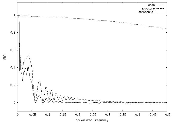
Dual-scan (dotted), dual-exposure (solid), and dual-structure (dashed) Fourier ring correlations (FRC) for a single micrograph from data set 1 (defocus = 2μ).

Using equation 4, the FRCs were converted to SSNRs, which are shown in Fig. 3 for micrographs from the first and second data sets (panels a and b, respectively). In Fig. 3a (defocus 2μ) the SSNR_{true_scan} is off the vertical scale. Because the SSNR_{true_scan} was so large, the SSNR_{true_exp} was virtually identical with SSNR_{comp_exp}, so the figure’s true exposure plot (solid line) corresponds to both composite and true exposure (SSNR_{comp_exp} and SSNR_{true_exp}). The dotted line (comp structural) and dashed line (true structural) correspond to composite and actual structural SSNR, respectively. SSNR_{true_exp} and SSNR_{true_scan} were obtained from the FRCs of the double experiments following the same logic as the corresponding SNRs (see above). The true structural SSNR has higher amplitude than the true exposure SSNR at low frequencies, except where the CTF is zero, out until around 1/8 Å⁻¹, after which it essentially falls to zero. This indicates that in this data set the structural noise is greater than the shot noise. The micrographs at the other three defoci in this data set gave similar results.

Figure 3.

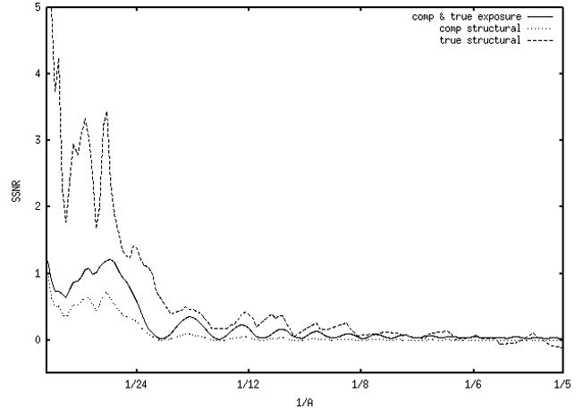
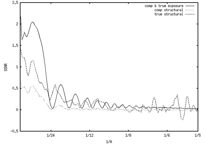
SSNRs computed from FRCs. (a) Data from a defocus group from data set 1 (2μ). The scan SSNR (not shown) is in the thousands, off the vertical scale. Due to the very high scan SSNR, the true-exposure SSNR is virtually identical to the composite-exposure SSNR, thus the solid line corresponds to both SSNR_{comp_exp} and SSNR_{true_exp}. The true structural SSNR (dashed line) is derived from both the composite-exposure SSNR and composite-structural SSNR (dotted line). (b) A defocus group from data set 2 (3μ). In (a) and (b), as well as in all following figures, 1/5 Å⁻¹ corresponds to 0.24 normalized (Nyquist) spatial frequency units in Figure 2.

Fig. 3b presents the same information for a micrograph from data set 2 (defocus 3μ). The results are similar except that the true structural SSNR (dashed line) stays below the shot noise SSNR at low frequencies. It has some positive regions that appear related to CTF oscillations out to around 1/10 Å⁻¹, after which it fluctuates around the zero line, due to the composite structural SSNR (dotted line) being zero above this frequency. The true structural SSNR takes on negative values at frequencies where the composite structural line, being somewhat noisy, dips below the zero line. The micrographs at the other three defoci in this data set gave similar results. Wherever SSNR dips below zero, a physical impossibility, it is the result of numerical or measurement errors.

Fig. 4 shows the true structural SSNR of the four defocus groups averaged together for the two data sets (panels a and b, respectively). Points corresponding to minima in the respective CTFs were excluded from the average. For the first data set in Fig. 4a, the average structural SSNR decreases approximately linearly from around 4 to around 0.2 (at 1/15 Å⁻¹). There is some information from 1/15 Å⁻¹ to around 1/8 Å⁻¹, after which the SSNR fluctuates around zero. Although lower in amplitude, the average structural SSNR for data set 2 in Fig. 4b is quite similar. It decreases approximately linearly from around 1 to zero at 1/15 Å⁻¹, beyond which it displays some frequency information until around 1/8 Å⁻¹, after which it fluctuates around zero. For comparison, the insets in Figures 4a and 4b give some estimate of the particle “signal”: power spectra of representative class averages from four defocus groups are shown, along with the averaged envelope function (dotted lines).

Figure 4.

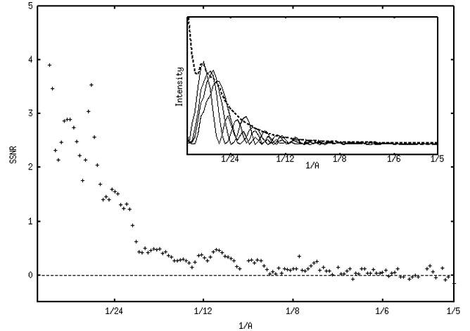
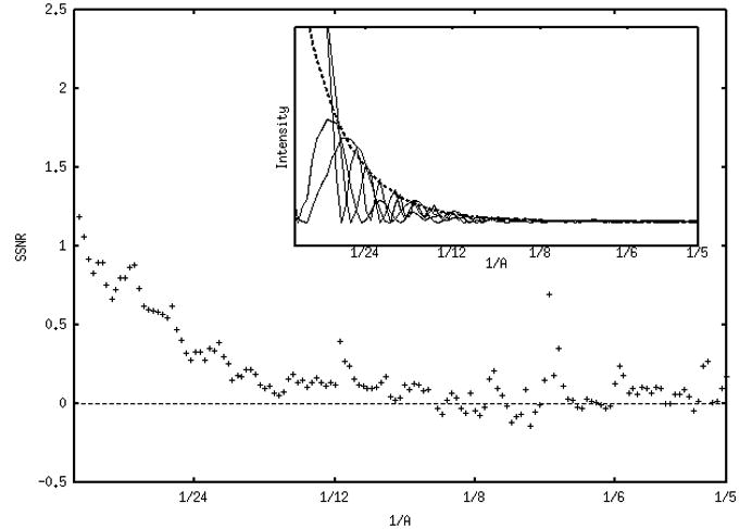
Average “true” structural SSNR of all four defocus groups (1μ, 2μ, 3μ, 4μ) for data set 1 (a) and set 2 (b). Note that the SSNR scale in (b) is expanded. Beyond 1/5 Å⁻¹ the behavior of the data becomes very unstable. Insets in both panels show the power spectra of representative class averages for four defocus groups (solid lines), along with the averaged envelope function (dotted lines). The envelopes were determined either using SPIDER’s TF ED operation, or by fitting the maxima with an exponential function using gnuplot.

Discussion and Conclusion

SNR Measurements

At the outset, the measured values of true SNRs for the two data sets are quite plausible: 27, 57 for scanning, 0.1, 0.09 for low-dose exposure of the same motif, and 1.4, 0.6 for reproducibility of a structure. The measurements confirm that the low SNR of low-dose micrographs is almost entirely due to the low reproducibility of the optical density distribution arising from the combined effect of shot noise and grain distribution in the emulsion. Errors in the particle alignment algorithm in SPIDER may also result in underestimation of the structural SNR. Finally, the underestimation of the dual-exposure SNR can result from slight misalignments between the two micrographs. The alternating display of particle image arrays (see Methods) suggested that this error was minor.

To get a perspective on the value for the structural SNR, we recall that the SNR in this case compares the variance of the signal due to the components of the object that are exactly reproducible with the variance of the noise, i.e., of those components of the object that are not reproducible. Conformational changes due to radiation damage, conformational differences from one structure to the next due to flexibility of peripheral components, and the differing structures of the matrix surrounding and supporting the molecule would all be counted as irreproducible. (The first of these irreproducible effects is actually contained in the double-exposure experiment, contributing toward the noise (SNR = 0.1) measured there, but there is no way to disentangle it from the shot noise using our cross-correlation strategy.) Considering the fact that there are three sources of structural noise, it is not surprising that signal and noise variances are in the same range.

Since the conformational variability of the ribosome in the two cases is not markedly different, as judged by the quality of 3D reconstructions (Valle et al., 2003; Taylor et al., 2007) the fact that the structural SNRs for different datasets differ by as much as a factor of 2 means that the attributes of the background can vary substantially: ice thickness and the thickness and texture of the added carbon film are possible factors. (More about this in the section on SSNRs which bear out the same discrepancy.)

It may seem surprising at first that the true structural SNR as measured by comparing images affected by the CTF varies so little as the defocus is changed, especially for the 70S dataset. However, both the reproducible and irreproducible components of the object are in fact identically affected by the CTF, which means that the ratio should theoretically remain constant as the defocus is varied.

SSNR Curves

In the curve measured for shot noise (“comp & true exposure”, Fig. 3) we see a steep falloff at first, then oscillations resulting from the CTF over the remainder of the range. The CTF signature is due to the fact that the exposures compared are not by a uniform beam, but by a distribution of electrons spatially modulated by the image of the identical object, which is affected by the same CTF. (The term “identical” has to be used with a grain of salt, since the first exposure will inevitably affect the structure somewhat; however, within the spatial frequency range examined (see below), these effects should be minor.)

The most striking difference between the two data sets is the reversal in the ratio of the true structural SSNR and true exposure SSNR at low frequencies (below approx. 1/15 Å⁻¹). In Fig. 3a the structural SSNR (dashed line) is above the exposure SSNR (solid line), indicating that the shot noise exceeds the structural noise in this range, as it does throughout the entire spatial frequency range with minor infractions. In the same spatial frequency range, in Fig. 3b, the exposure SSNR is much higher than the structural SSNR, indicating that now the structural noise prevails. Intuitively, if the composite exposure and composite structural SSNRs are similar, this means the shot noise SSNR is making a relatively small contribution, and the composite structural SSNR is composed of a larger proportion of the actual, true structural SSNR. Conversely, when the exposure SSNR is quite high compared to the composite structural SSNR, as in Fig. 3b below 1/24 Å⁻¹, it means the composite SSNR has a large contribution from the shot noise, and less so from the true structural SSNR.

The lower structural SSNR in the second data set could be due to any of the sources of the structural SNR: radiation damage, molecular conformational variability, and the surrounding carbon and ice matrix. If radiation were altering the molecules, we would expect to see changes in the particles between the two exposures. However, the cross-correlation coefficients for pairs of dual-exposure particle images is slightly higher for the second data set (see ρ_exp in Tables 1 and 2), indicating the particle images are retaining their similarity. As for conformational variations, the 80S•eEF2•GDPNP-Sordarin ribosome specimen is known to be quite stable (Taylor et al., 2007). This suggests the superposed carrier structure of ice and carbon is the principal source of the difference in structural noise seen between the two data sets in this study.

We interpret the initially high values in the true structural SSNR for all defocus groups (Figs. 3, 4) as an indication of high agreement in the overall shape of the molecule. The average true structural SSNR (Fig. 4) decreases approximately linearly in the range of 1/100 Å⁻¹ to around 1/15 Å⁻¹ for both data sets. From 1/15 Å⁻¹ to around 1/8 Å⁻¹, there are fluctuations in the curves that appear to correspond to the CTF. At higher frequencies the average structural SSNR is essentially zero, except where instabilities in equation 2 result in positive and negative peaks, with increasing divergence and fluctuation of the data beyond 1/5 Å⁻¹ (not shown).

Creation of Phantom Dataset

Our study has shown that to be realistic, phantom image data required for the testing and validation of new approaches to classification must include a structural noise term of a size roughly matching the signal. This noise portion gives rise to an image noise component that is unrelated to the object yet CTF-dependent. In the creation of phantom data, the noise term needs to be added to the projection of the 3D model structure, and the resulting “contaminated” image then needs to be subjected to the CTF before the shot noise and any noise from subsequent sources are added. In this context, it should be noted that recently, Zeng et al. (2007) also included a CTF-dependent noise contribution in a model of EM images derived from two-dimensional crystals.

A simulated dataset with structural heterogeneity was computed according to the measured SNR values reported in this work. Two density maps of the 70S E. coli ribosome complexes in different conformations were used to generate the data. These reconstructions had been previously obtained (Scheres et al. 2007) using a maximum likelihood-based classification from ~90,000 cryo-EM images of a heterogeneous sample of ribosome complexes (original source: Måns Ehrenberg, Uppsala). Map #1 represents the ribosome bound with three tRNAs at the A, P, and E sites, while map #2 represents an EF-G•GDPNP-bound ribosome with a deacylated tRNA bound in the hybrid P/E position. Besides differences in the binding of the ligands, the two maps also reflect differences in the ribosomal conformations: map #1 represents the normal conformation, while map #2 represents the ratcheted conformation (i.e., with the 30S subunit rotated counter-clockwise relative to the 50S subunit).

First, 5000 projection images were generated from each map with randomly distributed orientations (Eulerian angles ψ=0°; θ=0°–90°; ϕ= 0°–360°). Second, to simulate the structural noise, different realizations of random noise with zero-mean Gaussian distribution were added to all the projection images such that the resulting images had an SNR of 1.4 (seeα_{true_struct} in Table 3, column 1). Next, these noisy images were subjected to modulation by a contrast transfer function (CTF) that simulates the effect of the FEI Tecnai F30 Polara transmission electron microscope (Cs=2.26mm) operated in the bright-field mode at 300 kV and 2 μ underfocus. Finally, another set of zero-mean Gaussian noise images were added to simulate the effects of shot noise and digitization noise, which brought the final SNR to 0.05 (see α_{comp_struct} in Table 3, column 1), in agreement with the SNR measurements. Fig. 5 compares a set of such simulated images (bottom row) with some of the experimental images used in this study (top row), both at 2 μ defocus.

Figure 5.

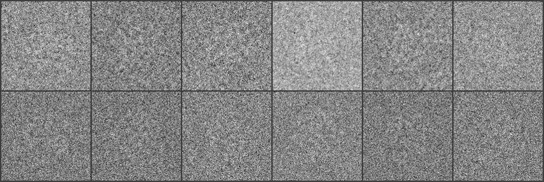
A comparison between the experimental images (top row) and simulated data (bottom row). Defocus = 2μ for both.

Conclusion

In this study we have modelled the image-formation process of low-dose TEM as a sequence of 3 stages which add noise to the signal: (1) the background of carbon and ice as well as variations in molecular conformation (structural noise); (2) fluctuations in the number of radiated electrons (shot noise); and (3) digitization, either by CCD or scanning following photographic development. At each stage, paired images were used to determine the cross-correlation coefficient, from which the signal-to-noise ratio was derived. Because the sub-processes occur in series, noise at each level is superimposed on noise from preceding levels, but its associated SNR may be disentangled by using the SNRs computed at previous steps. The measured digitization SNR proved very high, such that the imaging process was essentially limited by shot noise and structural noise alone. Dual-exposure images, which measured the contribution of shot noise, had an SNR of approximately 0.1 (for 300 kV, at 59,000X magnification). The structural SNRs measured for two ribosome data sets were 0.6 and 1.4, a difference that may reflect the varying contribution of the background matrix of ice and carbon. Structural noise, roughly the same magnitude as the signal, has the peculiar property that it is unrelated to the object of interest yet CTF-dependent. Inclusion of such a noise term makes the modeling of EM images more realistic.

A phantom data set has been constructed by adding a structural noise term, of a size corresponding to the experimentally measured SNR, to projected images of a density map (E. coli ribosome) before modification by the CTF and before the addition of ‘shot noise’. The phantom data set -- which should be useful for developing and testing classification procedures as the class membership of each image is known -- is available for download from the European Bioinformatics Institute (see below).

We also exploited the data collected to obtain estimates for the spectral signal-to-noise ratios (SSNRs), which depict the spectral distribution of the signal to noise ratio in the spatial frequency domain. The structural SSNR curves exhibited a rapid falloff to approximately 1/15 Å⁻¹, although some signal was evident out to 1/8 Å⁻¹. Interestingly, the curves showed that at very low spatial frequencies (less than 1/24 Å⁻¹) either shot noise or structural noise may predominate, probably depending on the physical properties of the specimen grid.

References

- Elad N, Clare DK, Saibil HR, Orlova EV. Detection and separation of heterogeneity in molecular complexes by statistical analysis of their two-dimensional projections. J Struct Biol. 2008;162:108–120. doi: 10.1016/j.jsb.2007.11.007. [DOI] [PubMed] [Google Scholar]
- Frank J. Three-Dimensional Electron Microscopy of Macromolecular Assemblies. Oxford University Press; New York: 2006. [Google Scholar]
- Frank J, Al-Ali L. Signal-to-noise ratio of electron micrographs obtained by cross-correlation. Nature. 1975;256:376–378. doi: 10.1038/256376a0. [DOI] [PubMed] [Google Scholar]
- Frank J, Radermacher M, Penczek P, Zhu J, Li Y, Ladjadj M, Leith A. SPIDER and WEB: processing and visualization of images in 3D electron microscopy and related fields. J Struct Biol. 1996;116:190–199. doi: 10.1006/jsbi.1996.0030. [DOI] [PubMed] [Google Scholar]
- Fu J, Gao H, Frank J. Unsupervised classification of single particles by cluster tracking in multi-dimensional space. J Struct Biol. 2007;157:226–239. doi: 10.1016/j.jsb.2006.06.012. [DOI] [PubMed] [Google Scholar]
- Kalinowski M, Herman GT. Classification of heterogeneous electron microscope projections into homogeneous subsets. Ultramicroscopy. 2008;108:327–338. doi: 10.1016/j.ultramic.2007.05.005. [DOI] [PubMed] [Google Scholar]
- Penczek PA. Three-dimensional spectral signal-to-noise ratio for a class of reconstruction algorithms. J Struct Biol. 2002;138:34–46. doi: 10.1016/s1047-8477(02)00033-3. [DOI] [PubMed] [Google Scholar]
- Scheres SH, Gao H, Valle M, Herman GT, Eggermont PP, Frank J, Carazo JM. Disentangling conformational states of macromolecules in 3D-EM through likelihood optimization. Nat Methods. 2007a;4:27–29. doi: 10.1038/nmeth992. [DOI] [PubMed] [Google Scholar]
- Scheres SHW, Nuñéz-Ramírez R, Gómez-Llorente Y, San Martin C, Eggermont PPB, Carazo JM. Modeling experimental image formation for likelihood-based classification of electron microscopy data. Structure. 2007b;15:1167–1177. doi: 10.1016/j.str.2007.09.003. [DOI] [PMC free article] [PubMed] [Google Scholar]
- Taylor DJ, Nilsson J, Merrill AR, Andersen GR, Nissen P, Frank J. Structures of modified eEF2-80S ribosome complexes reveal the role of GTP hydrolysis in translocation. The EMBO Journal. 2007;26:2421–2431. doi: 10.1038/sj.emboj.7601677. [DOI] [PMC free article] [PubMed] [Google Scholar]
- Unser M, Trus BL, Steven AC. A new resolution criterion based on spectral signal-to-noise ratios. Ultramicroscopy. 1987;23:39–52. doi: 10.1016/0304-3991(87)90225-7. [DOI] [PubMed] [Google Scholar]
- Valle M, Zavialov A, Sengupta J, Rawat U, Ehrenberg M, Frank J. Locking and unlocking of ribosomal motions. Cell. 2003;114:123–134. doi: 10.1016/s0092-8674(03)00476-8. [DOI] [PubMed] [Google Scholar]
- Zeng X, Stahlberg H, Grigorieff N. A maximum likelihood approach to two-dimensional crystals. J Struct Biol. 2007;160:362–374. doi: 10.1016/j.jsb.2007.09.013. [DOI] [PMC free article] [PubMed] [Google Scholar]