

Abstract
Opening angles (OAs) are associated with growth and remodeling in arteries. One curiosity has been the relatively large OAs found in the aortic arch of some animals. Here, we use computational models to explore the reasons behind this phenomenon. The artery is assumed to contain a smooth muscle/collagen phase and an elastin phase. In the models, growth and remodeling of smooth muscle/collagen depends on wall stress and fluid shear stress. Remodeling of elastin, which normally turns over very slowly, is neglected. The results indicate that OAs generally increase with longitudinal curvature (torus model), earlier elastin production during development, and decreased wall stiffness. Correlating these results with available experimental data suggests that all of these effects may contribute to the large OAs in the aortic arch. The models also suggest that the slow turnover rate of elastin limits longitudinal growth. These results should promote increased understanding of the causes of residual stress in arteries.
Keywords: artery, vascular mechanics, vascular development, wall stress, torus, tissue mechanics
1 Introduction
During the last decade, a number of mathematical models have been proposed for growing arteries (Taber, 1998; Rachev et al., 1998; Taber and Humphrey, 2001; Kuhl et al., 2006). Taken together, these models successfully capture many of the known characteristics of the adaptive behavior of arteries following perturbations in pressure and flow, such as changes in radius, wall thickness, and the opening angle (OA) associated with residual stress. Recently, some researchers have proposed models that focus on remodeling of the extracellular matrix (Driessen et al., 2004; Gleason et al., 2004; Hariton et al., 2007; Fonck et al., 2007), and we have developed a model that includes remodeling of collagen and elastin as well as growth of smooth muscle (Alford et al., 2007). For realistic distributions of these wall constituents, our model yields OAs that agree reasonably well with measured variations along the length of the rat aorta, with one notable exception — the aortic arch, where measured angles are considerably larger than in other regions (Liu and Fung, 1988).
Here, we extend our prior model for arterial growth and remodeling (G&R) (Alford et al., 2007) to investigate the reasons for the large OAs in the aortic arch. One obvious possibility is that they are caused by effects associated with longitudinal curvature, but other structural differences exist between the arch and the rest of the aorta. In addition, we explore the effects of longitudinal growth on the G&R behavior of arteries. Experiments have shown that the in vivo axial stretch of an artery changes as loading conditions change (Jackson et al., 2002), and Gleason and Humphrey (2005) showed that this adaptation is likely correlated with axial stress. However, to our knowledge, the effect of axial growth on residual stress has not yet been explored.
The results from our models indicate that longitudinal curvature increases OAs, but real aortas are not curved enough for this phenomenon to have a large effect. On the other hand, the models suggest that the relatively early elastin production that occurs in the arch during development (Davidson et al., 1986) can cause considerable increases in OA. Furthermore, a lower modulus for any of the wall constituents also increases the OA, and recent evidence suggests that elastin is less stiff in the arch region than it is downstream (Lillie and Gosline, 2007). Hence, it is likely that a combination of factors causes the relatively large OAs in the aortic arch. In addition, the models show that longitudinal growth can significantly affect opening angles. These results provide new understanding of the origins of residual stress in arteries.
2 Models and Assumptions
In this paper, we consider four thick-walled models for the aorta; two are straight cylinders (C1 and C2) and two are tori (T1 and T2). All models include circumferential and radial growth of smooth muscle cells, but other details differ. The main characteristics of the models are the following:
Model C1: Includes axial growth but not elastin production; used to study the effects of axial growth and media stiffness under homeostatic conditions at maturity. The ends of the cylinder are fixed at a specified axial stretch ratio.
Model C2: Includes axial growth and elastin production; used to simulate arterial development. Because increasing blood pressure drives expansion of the vascular bed in the embryo, the ends are assumed to be capped but free to move axially.
Model T1: Does not include axial growth or elastin production; used to simulate the arch of the aorta and examine the effects of longitudinal curvature on OAs. Axial growth is not included because G&R equilibrium cannot be achieved without elastin present.
Model T2: Includes axial growth and elastin; used to simulate the arch of the aorta and study the interaction between elastin stress and smooth muscle growth in a curved vessel.
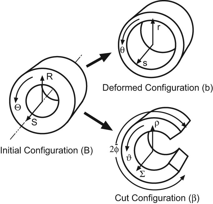
In the unloaded reference state (before any G&R), all models have circular cross sections. Reference geometry for the torus models is shown in Fig. 1; the cylinders have similar cross sections. For convenience, R, Θ, and S represent the radial, circumferential, and longitudinal coordinates in the reference configuration of all models, while r, θ, and s are the corresponding coordinates in the intact state at an arbitrary time t. For a torus, the circumferential direction is defined relative to the cross section. Moreover, we let A and B be the longitudinal radius of curvature and the radius of the lumen, respectively, in the reference state. At G&R equilibrium, the cross section also is assumed to be circular, and these radii become a and b, respectively (Fig. 1).
Figure 1.
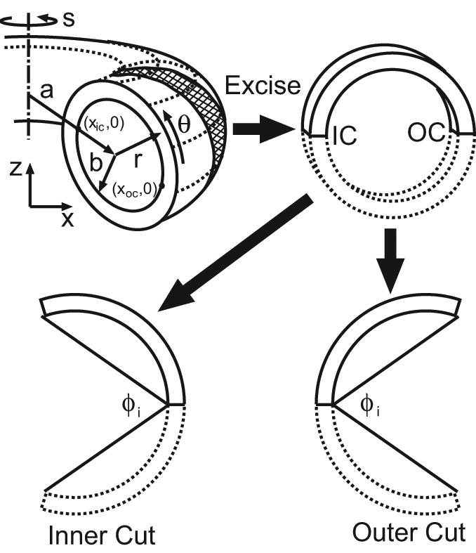
Schematic of torus model and opening angles. Geometry is shown at G&R equilibrium. Inner opening angles φi are shown for radial cuts at the inner curvature (IC) and outer curvature (OC) of the torus (see also Fig. 9A,B). Note: In this paper, the inner curvature always is located on the left side of the cross section.
Our analysis of G&R is based on the fundamental assumption that smooth muscle grows and collagen remodels, as these constituents strive to maintain their respective stresses at homeostatic values. However, elastin remodeling is neglected, as it turns over very slowly (order of years under normal conditions) once it is produced during development (Lefevre and Rucker, 1980; Davis, 1993). Previously, we have shown that a model based on these criteria yields OAs that depend on the relative thicknesses of the media and adventitia (Alford et al., 2007). This paper, however, focuses primarily on the aortic arch, which has a relatively thin adventitia. For simplicity, therefore, the present models are composed of a single layer, the media, which consists of a homogeneous mixture of smooth muscle, collagen, and elastin. In addition, noting the relatively rapid remodeling of smooth muscle and collagen (order of days to weeks), we assume that these constituents can effectively regain their homeostatic stresses on a short time scale compared to the relatively slow process of development. (Acute changes in loading are not considered here.) Thus, smooth muscle and collagen are lumped together into a single material (herein simply called “smooth muscle”) with an equivalent homeostatic stress.1 Hence, the artery wall in our models consists of a mixture of two constituents — smooth muscle (including collagen) and elastin.
Additional assumptions for the wall constituents include the following:
Smooth muscle is an incompressible (cylinder models), or nearly incompressible (torus models), pseudoelastic material growing at a rate that depends on the local circumferential stress σmθ and axial stress σms in the muscle and the fluid shear stress τw on the endothelium. Short-term adaptation involving muscle contractility is ignored.
Elastin sheets are composed of incompressible pseudoelastic fibers oriented originally in the circumferential (Θ) and longitudinal (S) directions. Elastin fibers are synthesized at specified times with the same initial stretch ratio (taken as 1.0 for simplicity). After production, the fibers do not turn over and are stretched or compressed by subsequent cell growth.
3 Theoretical Methods
The present formulation includes volumetric growth of smooth muscle according to the growth theory of Rodriguez et al. (1994) and elastin production adapted from the remodeling theory of Humphrey and colleagues (Humphrey, 1999; Humphrey and Rajagopal, 2003; Gleason et al., 2004). These theories are based on the concept of evolving natural (zero-stress) configurations for each tissue component. Consistent with the above assumptions, the arterial wall is taken as a mixture of smooth muscle cells, elastin, and water, with the cells assumed to be a growing scaffold on which elastin is synthesized. During deformation, all constituents are assumed to undergo the same strain at each point, i.e., the tissue is treated as a constrained mixture. The total Cauchy stress tensor in the mixture is given by
| (1) |
where φj is the volume fraction and σj the partial stress of constituent j. The volume fractions satisfy the relation φm + φe = 1. Water is assumed to be contained entirely within the smooth muscle/collagen phase.
3.1 Growth and Remodeling
To visualize how G&R is handled, it is helpful to consider a series of virtual configurations in which smooth muscle and elastin are treated separately (Fig. 2). The initial geometry B at time t = 0 is chosen as the reference configuration. Configurations also are shown for the current time t and an intermediate time τ (0 ≤ τ ≤ t).
Figure 2.
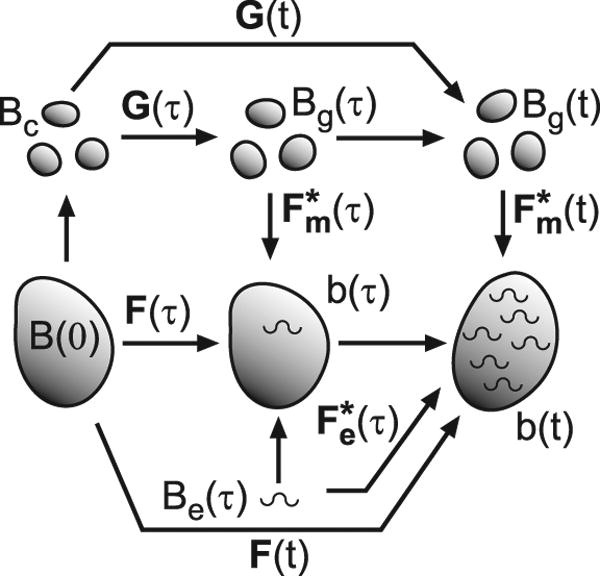
Configurations for growth and remodeling. Capital Bs represent stress-free configurations; lower case bs are configurations with stresses. For smooth muscle, the total deformation gradient tensor F is decomposed into a growth tensor G and an elastic deformation gradient tensor . Elastin produced at time τ undergoes the elastic deformation . See text for further details.
Suppose that the smooth muscle in B is dissociated into infinitesimally small pieces (Bc), e.g., individual cells, which then grow for an arbitrary time τ through the total growth tensor G (τ) to establish the zero-stress state Bg(τ) (Fig. 2). The pieces then are reassembled and external loads are added, as Bg undergoes elastic deformation (τ) to form configuration b (τ). These steps also apply at the current time t, and the total deformation of the smooth muscle at any time is given by
| (2) |
The field equations are written in terms of F, but the muscle stress depends of . The tensor G is determined from growth laws, as given below.
Arteries have three seemingly distinct growth modalities. In response to chronic changes in hemodynamic flow, arteries grow circumferentially to maintain the homeostatic shear stress on the endothelium (Langille et al., 1989). In response to chronic pressure changes, arteries grow radially, presumably to equilibrate wall stress (Matsumoto and Hayashi, 1996). Finally, in response to increased axial stress, arteries grow longer, possibly to equilibrate the stress along their axes (Jackson et al., 2002).
With these observations in mind, we set [G] =diag[λgr, λgθ, λgs], where the λgi are growth stretch ratios, and assume that the growth laws have the form
| (3) |
where Tθ, Tτ, Tr, and Ts are time constants, hat indicates homeostatic stresses, and dot denotes time differentiation. At G&R equilibrium, σmθ = σˆmθ, τw = τˆw, and σms = σˆms at all points in the artery.
Elastin production begins mid gestation, peaks near birth, and ceases in early infancy (Davidson et al., 1986). In previous work, we assumed that elastin is prestretched when it is created (Alford et al., 2007). But because elastin does not turn over, subsequent deformation during development likely overwhelms this initial stretch. For simplicity, therefore, we assume here that elastin fibers are created stress free at time τ (state Be (τ)) and then undergo elastic deformation (τ) to b(t), due external loading as well as growth of the artery. At any time, the stress born by elastin is given by the integral
| (4) |
where φ˙e (τ) is the volumetric rate of elastin production at time τ, and J = det F is the volume ratio.
3.2 Material Constitutive Laws
Let be the elastic deformation of constituent j (j = m, e) relative to its zero-stress state (Bg for smooth muscle and Be for elastin, Fig. 2). For a pseudoelastic material, the constitutive equations for the partial stresses are
| (5) |
where is the strain-energy density function for constituent j, and .
Smooth muscle is taken to be transversely isotropic with circumferentially oriented smooth muscle fibers. Hence, we take
| (6) |
where αm, βm, αf and βf are material constants and κ is the bulk modulus. In addition, is the modified first strain invariant relative to the stress-free configuration of the muscle (Bg), and p is a Lagrange multiplier for an incompressible material (J* → 1, κ → ∞) or a penalty variable for a nearly incompressible material. In the cylinder models (C1 and C2), smooth muscle is assumed to be incompressible, but, because the finite element package (COMSOL Multiphysics) requires some compressibility, the torus models (T1 and T2) are slightly compressible.2 Computed pressure-radius curves based on Eq. (6) show reasonable agreement with experimental data (results not shown).
Elastin is taken as a matrix of one-dimensional fibers in the local S-Θ plane, attached to the cells and assumed to be stress free at the time of synthesis. Because the stress-strain response of elastin is relatively linear at moderate levels of strain, we assume that it behaves as a neo-Hookean material. Hence, for uniaxial stretch of elastin fibers oriented in both the circumferential and longitudinal directions, the strain-energy density function is given by
| (7) |
where and are elastic stretch ratios (components of relative to Be), and αe is a material constant. Note that is based on the exact solution for a three-dimensional fiber, rather than a one-dimensional fiber.
4 Numerical Methods
4.1 Cylinder Models
The governing equations for G&R of a cylindrical artery are given in the Appendix. With G = I at t = 0, those equations and the growth and remodeling laws, Eqs. (3) and (4), were integrated via finite differences using a MATLAB program. Homeostatic solutions were obtained by integrating in time until the solution reached steady state. After a solution was found for the loaded vessel, G was held fixed while plane-stress equations were solved for the unloaded artery to obtain residual stresses and for the cut artery to obtain opening angles. Details of the solution procedure are provided in Taber (1998), Taber and Humphrey (2001), and Alford et al. (2007).
Two types of end conditions are considered. For a mature artery at homeostasis (model C1), the ends are fixed and the axial stretch ratio λs is specified. For a developing artery (model C2), the ends are capped but free to move axially. In this case, λs is an additional unknown to be determined using the axial equilibrium equation (A.4).
For simplicity, the homeostatic model C1 does not include elastin, while model C2 includes elastin produced during a specified period of development. Davidson et al. (1986) found that elastin synthesis progresses distally along the porcine aorta, peaking around birth in the arch region, one to two weeks later in the thoracic aorta, and three weeks later in the abdominal aorta. At time t = 0, we assume that the aorta is composed entirely of smooth muscle (φm = 1, φe = 0). Then, consistent with the data of Davidson et al. (1986), we specify elastin production according to the relation
| (8) |
where ton and toff are the times at which elastin production begins and ends, respectively. The peak production time is , and φe max is the total volume fraction of elastin for t ≥ toff (with φm = 1 − φe). Curves for three simulations are shown in Fig. 7A. Time is normalized such that t = 0 is the time at which blood pressure begins to develop in the artery and t = 1 is the time of birth.
Figure 7.
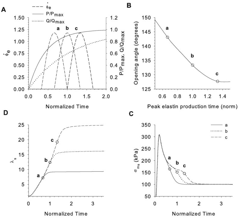
Effects of elastin production time on opening angles in cylinder model C2. (A) Pressure P, flow rate Q, and three example elastin production-rate curves (a, b, c) are plotted as functions of time during development. Time is normalized by the time of birth. (B) Opening angle plotted as a function of peak elastin production time. (C) Axial stretch ratio plotted as a function of time for cases a, b, and c. (D) Axial stress of smooth muscle at inner radius of artery plotted as a function of time for cases a, b, and c. Circles in B–D indicate the peak elastin production time for cases a, b, and c.
Pressure and flow oscillate during the cardiac cycle, but on a much shorter time scale than G&R. Hence, we assume that G&R depends on average loads. At t = 0, pressure (P) and flow rate (Q) are both set equal to zero. During development, average pressure and flow increase with time by
| (9) |
where Pmax and Qmax are the mature values of pressure and flow rate in the artery and γP and γQ are constants (see Fig. 7A). We assume that the average blood flow can be approximated by Poiseuille flow, giving an average endothelial shear stress
| (10) |
where μ is the viscosity of blood and ri is the deformed lumen radius. Because the value of τw is small compared to the pressure, the fluid shear stress is used in the growth law, but its effect on deformation is ignored.
In the cylinder models, the artery wall is taken as incompressible (κ = ∞) and, unless otherwise noted, the model parameters are
| (11) |
where time and the time constants are normalized relative to the time of birth.
4.2 Torus Models
The aortic arch is represented by a nearly incompressible pressurized torus (Fig. 1). The solution for inflation of a curved tube depends on θ (Kydoniefs and Spencer, 1965; Hill, 1980). For tori with large radii (A ≫ B, a ≫ b), the solution approaches that for a straight tube, but as the toroidal curvature tightens (A/B decreases), the circumferential stress at the inner curvature increases while the stress at the outer curvature decreases (Fig. 3). We speculated that this curvature effect is responsible for the higher OAs seen in the arch of the aorta, compared to the straighter distal regions. To test this hypothesis, we developed a stress-dependent growth model for a torus using COMSOL Multiphysics (v 3.3; Comsol, Inc.).
Figure 3.
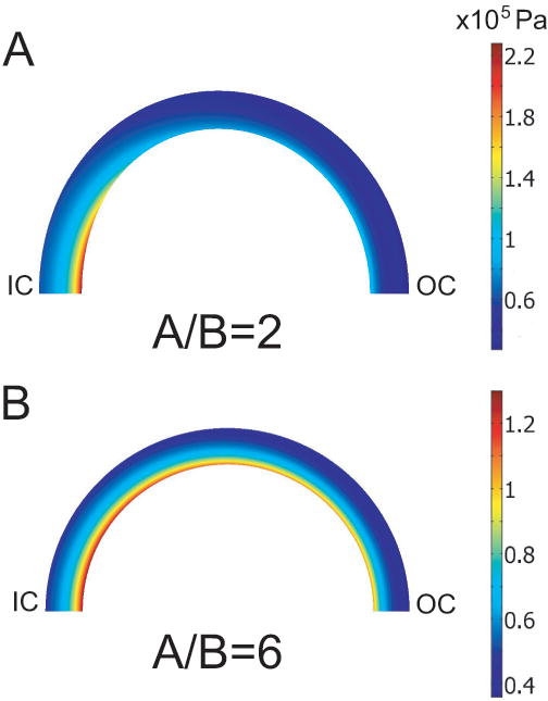
Circumferential Cauchy stress distributions in pressurized torus. (G&R is not included.) As the curvature increases (A/B decreases), a stress concentration develops near the inner wall at the inner curvature. IC = inner curvature; OC = outer curvature.
The computation is based on a nonlinear axisymmetric analysis relative to the toroidal axis, with only the top half of the torus considered and symmetry conditions applied. In COMSOL, traction boundary conditions must be transformed to follow the surface as it deforms. For an internal pressure P, Nanson's formula gives the traction vector
| (12) |
where N is the unit vector normal to the undeformed surface. The outer boundary is traction free.
The central dogma for arterial lumen maintenance is that arteries grow in response to chronic alterations in flow to return the endothelial shear stress toward a homeostatic value (Zamir, 1977). Numerical simulations have shown, however, that the fluid shear stress in the aortic arch is significantly nonuniform (Shahcheraghi et al., 2002; Suo et al., 2007). Nevertheless, the shape of the pressurized lumen is actually quite circular (Moreno et al., 1998), and numerical studies have shown that luminal maintenance is necessary for a stable and robust model (Taber, 1998). Hence, we assume that the artery attempts to maintain a circular lumen with a certain homeostatic radius. The reasons for this are unclear, but perhaps a circular lumen helps prevent turbulent flow or promotes structural efficiency by reducing potential stress concentrations in the artery wall.
The second of Eqs. (3) implies that circumferential growth is controlled, in part, by a signal from the endothelium in response to the fluid shear stress τw. For a circular cylinder, τw has a single value in any given cross section, and all points in the wall respond to the same signal. As shown in Fig. 3, however, the lumen in a pressurized torus is not circular in general, and τw varies around the circumference, even if curvature effects on flow are ignored. Hence, a point in the wall would receive signals of different strengths from various points on the endothelium. To handle this situation numerically, we solve the diffusion problem for the signal concentration c and assume that the magnitude of the growth response depends on the local value of c, as governed by the equation
| (13) |
where ∇2 is the two-dimensional Laplacian operator in the deformed coordinate system of the cross section.
The moving boundaries for the diffusion problem were handled in COMSOL using the built-in arbitrary Lagrangian-Eulerian (ALE) method with Winslow smoothing. This technique computes a deformed mesh at each time step by solving Laplace's equation for the mesh displacements. The value of c at the endothelium is assumed to be proportional to the deviation of the lumen from circularity. Hence, for convenience, the boundary condition at the inner wall is taken as
| (14) |
where (x, z) is the deformed location of a point on the lumenal boundary and (xc, zc) is the location of the center of the lumen, defined by the coordinates (see Fig 1). The outer boundary is assigned a flux condition ∇c = 0.
With these assumptions, Eq (3)2 is modified as
| (15) |
where Tc is a time constant and cˆ is the target signal concentration, i.e., the desired lumen radius (rˆ). At G&R equilibrium, c = cˆ = rˆ at all locations in the artery. For model T2, Fig. 4 illustrates how the distribution of c evolves with time as the lumen becomes circular.
Figure 4.
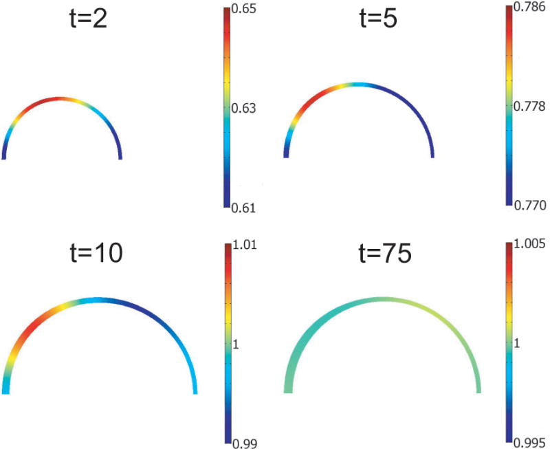
Diffusion of endothelial signal in torus model. Normalized signal c/cˆ is shown for four time points during development. As the model reaches G&R equilibrium, c uniformly approaches the target value cˆ (t = 75).
For computational convenience in computing residual stresses and opening angles, we represented the unloaded and cut artery slices as cylindrical sections using a pseudo-plane-strain analysis (Fig. 1). For the intact unloaded section, the horizontal diameter is a symmetric axis; for the cut section, one boundary along this axis is released. We enforced an average plane-stress condition by setting the average axial stress to zero, i.e.,
| (16) |
where A is the cross-sectional area of the excised section. In COMSOL, Eq. (16) is integrated for each iteration, and the uniform axial stretch ratio λs is determined by solving the auxiliary equation
| (17) |
where ν is a constant. The variable λs reaches a constant value when σ̄s = 0.
The governing equations were solved via quasi-static analysis. (For details on how growth is included in COMSOL, see Taber (2007)). At t = 0, we set P = 0 and G = I. The pressure was increased linearly in time to Pmax at t = 10. The smooth muscle was allowed to grow until σmθ = σˆmθ, σms = σˆms and c = cˆ. To calculate the unloaded and cut configurations, the values for Fg in the torus model were imported into the pseudo-plane-strain model. Opening angles were calculated for cuts at the inner curvature and the outer curvature of the torus (see Figs. 1 and 9A,B).
Figure 9.
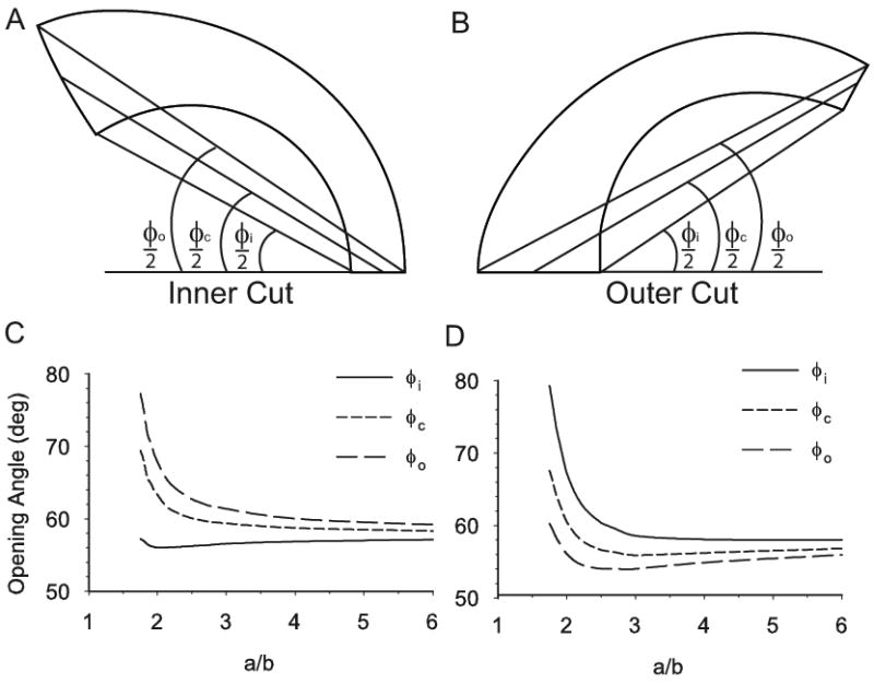
Effect of longitudinal curvature on homeostatic opening angles in torus model T1. Due to inhomogeneous wall thickness, opening angles measured at the inside φi), center (φc), and outside (φo) of the wall are different. (A,B) Examples of opening angles for cuts at inner and outer curvature of vessel. Cut sections are given by the model. (C,D) Opening angles are plotted as functions of the normalized longitudinal radius of curvature a/b with b = 1.5 mm.
Unless otherwise noted, the model parameters used in the torus models are
| (18) |
To evaluate the accuracy of our finite element analysis, results from model C1 with fixed ends were compared to those from an equivalent plane-strain COMSOL model. Even though model C1 is incompressible and the COMSOL model is slightly compressible, the models yield nearly identical residual stresses and OAs for various specified growth distributions, lumen size, and target stresses (results not shown).
5 Results
5.1 Effects of Axial Growth on Opening Angles
The homeostatic cylinder model C1 was used to study how axial growth influences the OA. If axial growth is not included, the OA depends strongly on the magnitude of the axial stretch ratio λs (Fig 5A). Notably, the peak value (about 116°) occurs at the value of λs for which passive inflation of a tube without residual stress yields the largest circumferential wall stress (Fig 5B). Due to nonlinearities, when the value of λs is increased from 0.5 to 2.5, the stress peaks around λs = 1.6, where the largest OA also occurs. In contrast, if axial growth is included, the OA is unchanged by axial stretch (Fig 5A).
Figure 5.
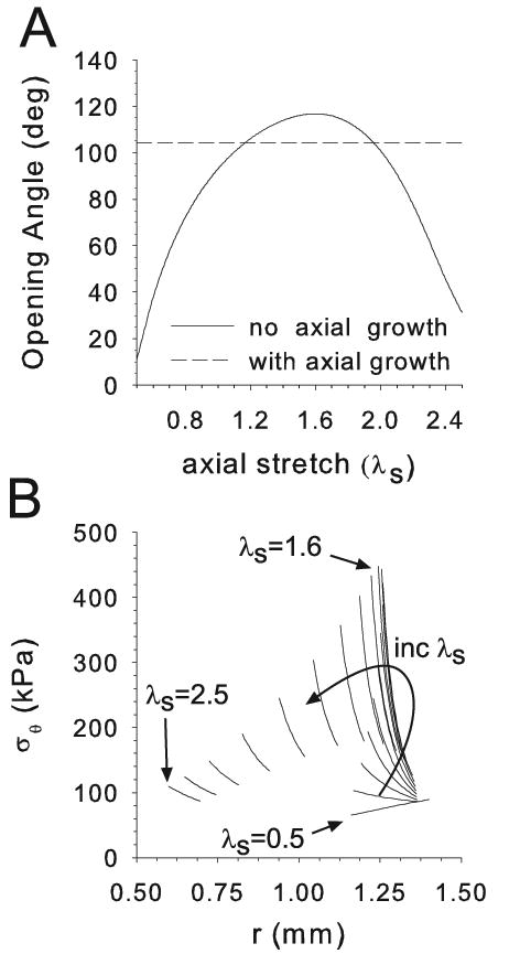
Effects of axial stretch in cylinder model C1. (A) Homeostatic opening angle plotted as a function of axial stretch ratio λs, with and without axial growth. (B) Transmural circumferential stress distributions in pressurized cylinder (P = 16 kPa) for various axial stretch ratios. The peak stress occurs at the same stretch ratio (λs ≈ 1.3 in this example) as the peak opening angle for no axial growth.
In model C1, the smooth muscle modulus αm greatly affects the OA (Fig. 6A). The OA becomes smaller as αm increases, regardless of the inclusion of axial growth. (Note: For a more direct comparison of modulus to opening angle, we set αf = 0 in Fig 6A only. However, if αf ≠ 0, the qualitative trend remains the same for variations in either αm or αf (results not shown)).
Figure 6.
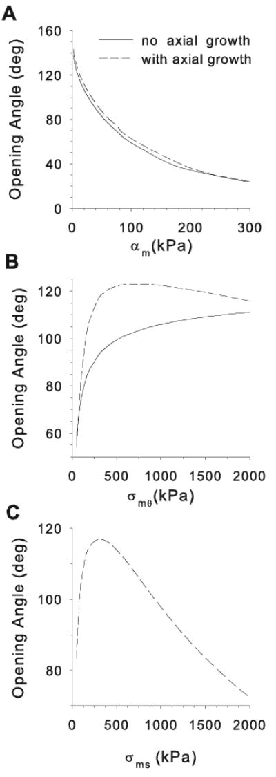
Effects of smooth muscle modulus (αm) and target stresses (σˆmθ and σˆms) on opening angle in cylinder model C1. Parameters are varied one at a time from the values αm = 10 kPa, σˆmθ = 300 kPa, and σˆms = 300 kPa. (A) Effects of αm with and without axial growth. (B) Effects of circumferential target stress with and without axial growth. (C) Effects of axial target stress with axial growth.
With no axial growth, opening angles increase monotonically with the value of the circumferential target stress σˆmθ (Fig 6B). (Note that the homeostatic wall thickness decreases with σˆmθ.) When axial growth is included, however, the OA reaches a peak around σˆmθ ≈ 600 kPa and then decreases for higher target stresses. A similar trend is seen when the axial target stress σˆms is varied, with the peak OA occurring when σˆms ≈ 300 kPa (Fig 6C). Qualitatively, these trends are the same if the muscle is considered isotropic (αf = 0) (results not shown).
5.2 Effects of Elastin Production Time
5.2.1 Opening Angles
During development, the peak elastin production rate moves as a proximal to distal wave along the aorta, and the total elastin production decreases with distance from the heart (Davidson et al., 1986). Our previous model accounts for the decreased elastin content along the aorta (Alford et al., 2007). Here, using model C2 for the developing aorta, we focus on the effect of elastin production time.
Simulations were run for a number of cases, three of which are highlighted in Fig. 7. In cases a, b, and c, elastin is synthesized before, during, and after the time of birth, respectively (Fig. 7A). The earlier elastin appears, the higher is the OA at G&R equilibrium (Fig.7B).
5.2.2 Axial Growth
According to model C2, elastin plays a crucial role in regulating arterial length. If elastin is never produced, the developing artery grows without bound. In addition, the length of the vessel (i.e., λs) reaches equilibrium soon after the peak elastin production rate occurs (Fig. 7C). At the same time, the onset of elastin production hastens the equilibration of the axial muscle stress σms (Fig. 7D).
5.3 Effects of Axial Curvature
5.3.1 Growth and Residual Stress
As longitudinal curvature decreases (toroidal radius of curvature increases), the circumferential Cauchy stress3 due to inflation approaches θ-independence, similar to that in a straight tube. As the curvature increases, however, a stress concentration develops near the inner radius of the inner curvature of the tube (Fig. 3). Therefore, to bring the smooth muscle cells to their target stress, there must be a similar θ-dependent growth distribution. For model T2 (with elastin fibers and axial growth), this behavior is illustrated for tori of three different curvatures (Fig. 8). The three components of G are shown at G&R equilibrium, as well as the resulting circumferential residual stress in the unloaded torus. In the tubes with tighter curvature (a/b = 2.0, 3.4), radial and circumferential growth are distinctly higher at the inner curvature than the outer curvature. Correspondingly, the vessel wall is thicker at the inner curvature than at the outer curvature in both the loaded and unloaded section.
Figure 8.
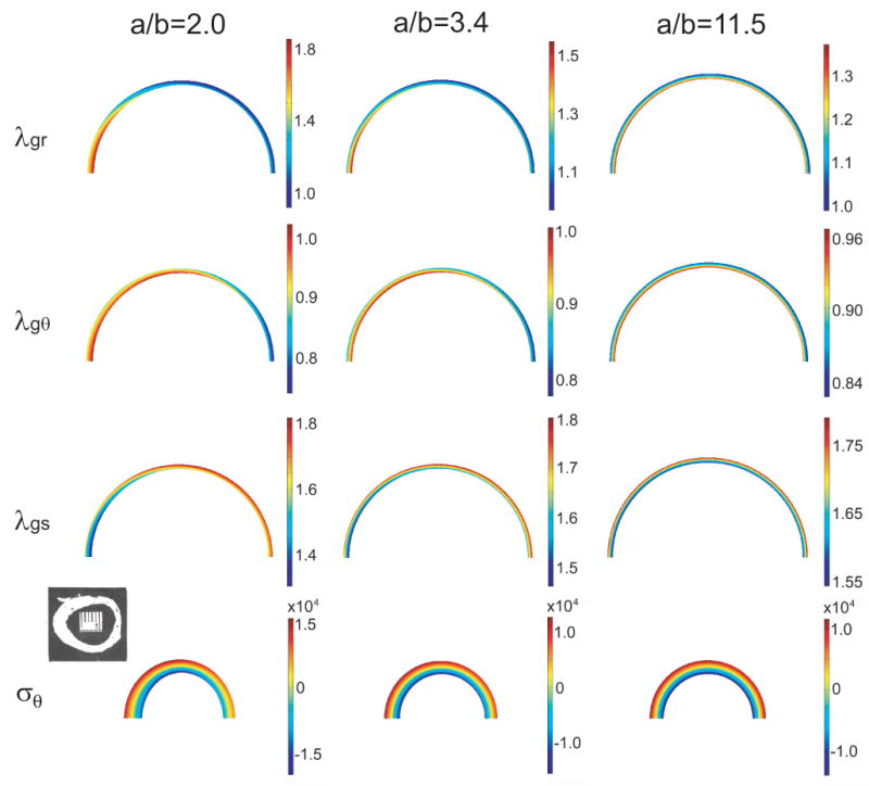
Growth and residual stress in torus model T2 at G&R equilibrium. Growth in the radial (λgr), circumferential (λgθ), and axial (λgs) directions (loaded artery) and circumferential residual stress (σθ, unloaded artery) are shown for three values of the normalized radius of curvature a/b. For each case, b = 1.5 mm at G&R equilibrium. Note: In the reference configuration, the corresponding values are A/B = 2.3, 4.0, and 13.3. Inset: Section of unloaded porcine aortic arch; reprinted from Han and Fung (1991) with permission of ASME.
If axial growth is included without elastin, the torus undergoes unbounded growth, never achieving the target stress. This response is consistent with the cylindrical model C2 for the developing artery.
5.3.2 Opening Angles
Liu and Fung (1988) found that OAs in the rat aorta depend on the location of the radial cut. Here, two cuts are considered for the torus model T1 (no elastin or axial growth) — one at the inner curvature (inner cut) and one at the outer curvature (outer cut) (see Fig. 1).
Because wall thickness in the unloaded section is not uniform, it is important to note how the OA is defined. Figure 9A,B shows three different opening angles for inner and outer cuts of model T1. The inner angle φi is the traditionally measured opening angle (Chuong and Fung, 1986). The outer angle φo and the central angle φc are defined similarly, as shown. The homeostatic value of each of these OAs is plotted as a function of the normalized longitudinal radius of curvature (a/b) (Fig. 9C,D). For the inner cut, the traditional OA, φi, changes little, while the other angles increase sharply for large curvatures (small a/b) (Fig. 9C). For the outer cut, the opposite effect is seen, as φi increases the most (Fig. 9D). Hence, how the OA is measured is extremely important.
For a vessel of uniform thickness, all of the OAs would have the same value. But because the inner curvature is thicker than the outer curvature, the traditionally measured OA (φi) may not accurately describe the deformation of the section following a transmural cut. For the inner cut, the inner angle likely underestimates the subsequent unbending, while for the outer cut, it likely overestimates the unbending. Although experimentally cut edges are not always clean, we recommend using the central angle (φc), which is an approximate average of the three angles.
The behavior illustrated in Fig. 9C,D seems to be quite robust. For realistic material parameters and target stresses, the curves in Fig. 9 change very little qualitatively for both models T1 and T2 (results not shown).
6 Discussion
It long has been known that arteries adapt to their physical environment. Macroscopically, geometric adaptations to changes in loading are readily observed. In response to acute changes in hemodynamic flow rate, many arteries contract or dilate to maintain a desired fluid shear stress on their endothelia (Johnson, 1980; Holtz et al., 1984). If the altered flow persists, the wall grows and remodels to maintain the new geometry as the smooth muscle tone returns toward normal levels (Langille et al., 1989). In cases of sustained hypertension, arteries thicken and stiffen, presumably to maintain homeostatic values of wall stress (Fung and Liu, 1991; Matsumoto and Hayashi, 1996). Arteries also grow and remodel in response to forces applied along their longitudinal axes (Jackson et al., 2002).
On the subcellular level, a number of biomolecules are expressed in response to changes in pressure or endothelial shear stress. These include, but are not limited to, nitric oxide, prostacyclin, endothelin-1, transforming growth factor-1, and fibroblast growth factors 1 and 2 (Humphrey, 2002). Further, arterial smooth muscle cells rapidly reorganize their focal adhesions and stress fibers in response to loading beyond their homeostatic stress state (Na et al., 2007). On the genetic level, Huang et al, (2001) showed that the upregulation of a number of genes in arterial tissues correlates directly with induced hypertension.
In addition to these gross macroscopic and fine intracellular adaptations, artery growth and remodeling can also be characterized as a response to variations in the local stress state of the artery wall. Recently, Dajnowiec et al. (2007) demonstrated that arterial growth is influenced by local stresses in the wall by showing that endothelial and smooth muscle cells divide preferentially in the direction of the highest applied force. The opening angles studied in this paper provide an indirect measure of this local adaptation.
The present study extends our previous model for arterial G&R (Alford et al., 2007) to explore two unanswered questions (1) What is the cause of the relatively large OAs that occur in the arch of the rat aorta? (2) How does longitudinal growth affect the response?
6.1 Opening Angles in the Aortic Arch
Opening angles vary substantially from artery to artery and from region to region within a single artery. Along the aorta, for example, OAs can vary by as much as 200° (Liu and Fung, 1988). In rat and porcine aortas, the arch region has significantly higher OAs than the more distal thoracic and abdominal regions (Liu and Fung, 1988; Han and Fung, 1991). Recently, we presented a model that includes realistic transmural and axial distributions of smooth muscle cells, elastin, and collagen (Alford et al., 2007). This model yields OAs that agree reasonably well with experimental measurements in all regions along the length of the rat aorta, except for the arch, where the predicted values are about 100° too low.
In this paper, we examined two possible causes for the elevated opening angles in the arch — longitudinal curvature and the timing of elastin synthesis during development. In our models, both effects elevate the OA, but not to the degree seen in the experiments.
Longitudinal curvature, to one extent or another, is present in all arteries. Even arteries that are considered relatively straight, like the carotids, are transiently curved by natural movements. The present study focuses on arteries with large intrinsic curvature. Our application is the arch of the aorta, but this analysis also could apply to other highly curved arteries such as those in the Circle of Willis.
The torus models predict that the central OA changes relatively little until the longitudinal curvature becomes very large, and then it begins to increase dramatically (a/b ≲ 2, Fig. 9C,D). Liu and Fung (1988) found that the radius of curvature of the excised rat aorta is no smaller than about 3 mm, with a lumen radius being about 1 mm, giving A/B = 3. When a model with these dimensions is inflated at G&R equilibrium, the loaded ratio a/b reduces to about 2.2, putting it near, but not quite on, the steep portion of the curve shown in Fig. 9. Hence, the actual curvature of the aorta likely accounts for only a small portion of the elevated OAs in the arch. On the other hand, the model correctly predicts the wall thickening at the inner curvature of the arch, as found by Han and Fung (1991) in the porcine aorta (Fig. 8, lower left).
In model C2 for the developing aorta, earlier elastin production leads to higher OAs (Fig. 7B). This behavior follows from the assumption that elastin does remodel after its initial synthesis. As the artery wall thickens during development, the elastin created near the outer radius is stretched further than that near the inner radius, thereby creating a net moment that bends the section open after a radial cut. The earlier the elastin is synthesized, the greater the transmural stress gradient and moment, and thus the higher is the OA. However, the increase due to this effect is only about 15°-20°.
Hence, according to our models, the effects of neither longitudinal curvature nor the timing of elastin production are great enough to explain completely the relatively large opening angles found in the aortic arch. Another possibility is suggested by the recent study of Lillie and Gosline (2007), who found that the modulus of elastin in the pig aorta increases with distance from the heart. Our results show that decreasing smooth muscle/collagen modulus (Fig. 6A) or elastin modulus (not shown) can lead to significant increases in OAs. A lower stiffness in the arch, therefore, could explain the discrepancy. In the end, all of these effects may contribute to the large OAs in the arch.
To repeat, Fig. 6A shows that the OA decreases as the wall modulus increases. Moreover, the curve for no axial growth in Fig. 6B shows that the OA also decreases as the circumferential target stress drops. For a given pressure and radius, simple equilibrium considerations (i.e., Laplace's law) indicate that lower circumferential wall stress requires a thicker wall. Both of these effects — an increased wall modulus and a thicker wall — are associated with a higher wall stiffness. Consequently, when the artery is cut, the amount of bending due to the release of residual stress is less, leading to a smaller OA. This possible relation between wall stiffness and OA warrants further study.
6.2 Axial Growth in Arteries
The most notable result from our study of axial growth is that, according to our model, the length of a developing artery would grow without bound without the introduction of a constituent with a very slow turnover rate. Elastin seems the likely candidate for this growth regulator. This result agrees with experimental evidence in mice showing that disruption of elastogenesis results in long tortuous, i.e., buckled, arteries (McLaughlin et al., 2006). Consistent with this idea, model C2 predicts that arteries with delayed elastin production grow longer than arteries in which elastin is produced early in development (Fig. 7C).
Our models also indicate that, if axial growth does not occur, then the OA depends strongly on the magnitude of the axial stretch in vivo (Fig. 5A). If axial growth occurs, however, the stretch has no effect on OA. The reason for this is that, if axial growth is included, then the homeostatic state of stress is independent of the length of the artery, as all stress components are at their respective target values.
6.3 Limitations
As with any model, the underlying assumptions could affect the accuracy of the results. A key assumption is that muscle and collagen maintain uniform target stresses under homeostatic conditions. This assumption warrants further testing, but it is consistent with our previous models, which have generally produced results in reasonable agreement with available experimental data (Alford et al., 2007).
In all of the models presented here, smooth muscle and collagen are treated as a single composite material characterized by a relatively simple strain-energy density function. We performed some simulations that indicate that this is a reasonable assumption during the relatively slow process of G&R (results not shown), but modeling adaptation to acute changes in loading requires treating muscle and collagen as separate constituents (Gleason et al., 2004; Alford et al., 2007). Further, we have assumed that the distributions of collagen, elastin and smooth muscle cells do not vary circumferentially. Such variations would affect growth and remodeling patterns and could account for changes in opening angles.
We have ignored the complex pressure and flow patterns that occur in the aortic arch, due to its curvature as well as the junctions with the carotid arteries (Kilner et al., 1993). Branches also affect the state of stress in the vessel wall (Zhao et al., 2002). Moreover, the G&R behavior is treated phenomenologically without taking into account gene and protein expression. All of these issues are obviously important, but outside the scope of this paper.
It is important to note that the elevated OAs in the arch are not conserved across all species. Rat and pig show this trend, but mice and humans do not and, in fact, show relatively little variation in OA along the entire length of the aorta (Saini et al., 1995; Guo and Kassab, 2004). A detailed study comparing the microstructure of different species could help to elucidate the source of OA variations. It is also important to note that opening angles do not completely characterize the residual stress state of an artery. It has been shown, for example, that a second, circumferential cut in the wall yields additional stress relief (Vossoughi et al., 1993; Greenwald et al., 1997). We have not addressed this issue here, but two-cut opening angles have been examined in our previous models (Taber and Humphrey, 2001; Alford et al., 2007). A comprehensive study of two-cut opening angles in the arch compared to straighter sections of the aorta could be valuable in helping to determine the source of the elevated opening angles in the arch.
In conclusion, the physiological reasons for the variations in residual stress and opening angles that occur along the aorta are not yet completely understood. Our models show that opening angles are affected by various factors, including curvature and wall stiffness. They also indicate that the timing at which elastin is introduced into the artery during development has important implications on the growth response to pressure loads. We hope that this information provides new understanding of growth and remodeling in arteries that can be used by tissue engineers as they design methods to construct replacement blood vessels.
Acknowledgments
This work was supported by NIH grants R01 GM075200 (LAT) and R01 HL64372 (PI: Jay Humphrey). We thank Guy Genin for suggesting the diffusion control of lumen size and shape used in the analysis.
Appendix A: Field Equations for a Cylinder
Intact Artery
Models C1 and C2 are thick-walled cylinders with fixed ends and capped ends, respectively, subjected to an internal pressure P. In the initial configuration B, a point in the wall is located at the cylindrical coordinates (R, θ, S) (Fig 10). In the deformed configuration b, the location of the point is (r, θ, s). At a given time, the deformation from B to b is mapped by the relations
Figure 10.
Configurations for cylinder model. Growth, remodeling, and applied loads deform the cylinder from initial configuration B to deformed configuration b. When a transmural cut is made in the unloaded artery, the section springs open, yielding the cut configuration β.
| (A.1) |
where λ is the axial stretch ratio. The components of the total deformation gradient tensor F are given by
| (A.2) |
The equations of radial and axial equilibrium, respectively are
| (A.3) |
| (A.4) |
where the σi are Cauchy stress components, and ri and ro are the inner and outer radii of the deformed cylinder. The boundary conditions are σr(ri) = −P and σr(ro) = 0. For a cylinder with capped ends, λs is an unknown. For fixed ends, λs is specified, and Eq. (A.4) is not needed.
Cut Artery
To calculate the cut configuration β, we assume that the artery remains a circular sector (Fig 10). The deformation to β relative to the loaded configuration b is defined by
| (A.5) |
where (p, ϑ, Σ) are the coordinates of a point in β, Λ is the axial stretch ratio, and the OA φ is defined by φ = π − φ̄ (Taber and Humphrey, 2001). The associated stretch ratios relative the loaded state are given by
| (A.6) |
which satisfy the incompressibility condition λρλϑλΣ = 1. The radial force, axial force and moment equilibrium equations, respectively, are
| (A.7) |
where ρi and ρo are the inner and outer radii of the cut artery, respectively. The boundary conditions are σρ(ρi) = σρ(ρo) = 0.
Footnotes
This simplification was used because including collagen remodeling in the torus models increased computation time by more than an order of magnitude. To test the accuracy of this approximation, we ran some simulations with the cylinder models with and without separate collagen remodeling and found only minor differences for the problems in this paper.
The bulk modulus κ used in this study is several orders of magnitude greater than the material modulus. So in the compressible model, J* ≈ 1, and the pressure-radius curves for the cylinder models are nearly identical for the incompressible and slightly compressible cases (results not shown).
Cauchy stress is computed relative to convected base vectors. Thus, circumferential stress in the torus may not correspond to the circumferential direction in the reference configuration.
References
- Alford PW, Humphrey JD, Taber LA. Growth and remodeling in a thick-walled artery model: effects of spatial variations in wall constituents. Biomechanics and Modeling in Mechanobiology. 2007 doi: 10.1007/s10237-007-0101-2. in press. [DOI] [PMC free article] [PubMed] [Google Scholar]
- Chuong CJ, Fung YC. On Residual Stresses in Arteries. J Biomech Eng. 1986;108:189–192. doi: 10.1115/1.3138600. [DOI] [PubMed] [Google Scholar]
- Dajnowiec D, Sabatini PJ, Van Rossum TC, Lam JT, Zhang M, Kapus A, Langille BL. Force-induced polarized mitosis of endothelial and smooth muscle cells in arterial remodeling. Hypertension. 2007;50:255–260. doi: 10.1161/HYPERTENSIONAHA.107.089730. [DOI] [PubMed] [Google Scholar]
- Davidson JM, Hill KE, Alford JL. Developmental changes in collagen and elastin biosynthesis in the porcine aorta. Dev Biol. 1986;118:103–111. doi: 10.1016/0012-1606(86)90077-1. [DOI] [PubMed] [Google Scholar]
- Davis EC. Stability of elastin in the developing mouse aorta: a quantitative radioauto-graphic study. Histochemistry. 1993;100:17–26. doi: 10.1007/BF00268874. [DOI] [PubMed] [Google Scholar]
- Driessen NJB, Wilson W, Bouten CVC, Baaijens FPT. A computational model for collagen fibre remodelling in the arterial wall. Journal of Theoretical Biology. 2004;226:53–64. doi: 10.1016/j.jtbi.2003.08.004. [DOI] [PubMed] [Google Scholar]
- Fonck E, Prod'hom G, Roy S, Augsburger L, Rufenacht DA, Stergiopulos N. Effect of elastin degradation on carotid wall mechanics as assessed by a constituent-based biomechanical model. Am J Physiol Heart Circ Physiol. 2007;292:H2754–H2763. doi: 10.1152/ajpheart.01108.2006. [DOI] [PubMed] [Google Scholar]
- Fung YC, Liu SQ. Changes of Zero-Stress State of Rat Pulmonary Arteries in Hypoxic Hypertension. J Appl Physiol. 1991;70:2455–2470. doi: 10.1152/jappl.1991.70.6.2455. [DOI] [PubMed] [Google Scholar]
- Gleason RL, Humphrey JD. Effects of a sustained extension on arterial growth and remodeling: a theoretical study. J Biomech. 2005;38:1255–1261. doi: 10.1016/j.jbiomech.2004.06.017. [DOI] [PubMed] [Google Scholar]
- Gleason RL, Taber LA, Humphrey JD. A 2-D model of flow-induced alterations in the geometry, structure, and properties of carotid arteries. J Biomech Eng. 2004;126:371–381. doi: 10.1115/1.1762899. [DOI] [PubMed] [Google Scholar]
- Greenwald SE, Moore JEJ, Rachev A, Kane TPC, Meister JJ. Experimental Investigation of the Distribution of Residual Strains in the Artery Wall. J Biomech Eng. 1997;119:438–444. doi: 10.1115/1.2798291. [DOI] [PubMed] [Google Scholar]
- Guo X, Kassab GS. Distribution of stress and strain along the porcine aorta and coronary arterial tree. Am J Physiol Heart Circ Physiol. 2004;286:H2361–H2368. doi: 10.1152/ajpheart.01079.2003. [DOI] [PubMed] [Google Scholar]
- Han HC, Fung YC. Species Dependence of the Zero-Stress State of Aorta: Pig Versus Rat. J Biomech Eng. 1991;113:446–451. doi: 10.1115/1.2895425. [DOI] [PubMed] [Google Scholar]
- Hariton I, Debotton G, Gasser TC, Holzapfel GA. Stress-modulated collagen fiber remodeling in a human carotid bifurcation. J Theor Biol. 2007 doi: 10.1016/j.jtbi.2007.05.037. in press. [DOI] [PubMed] [Google Scholar]
- Hill JM. The Finite Inflation of a Thick-Walled Elastic Torus. Q J Mech Appl Math. 1980;33(Part 4):471–490. [Google Scholar]
- Holtz J, Forstermann U, Pohl U, Giesler M, Bassenge E. Flow-dependent, endothelium-mediated dilation of epicardial coronary arteries in conscious dogs: effects of cyclooxygenase inhibition. J Cardiovasc Pharmacol. 1984;6:1161–1169. [PubMed] [Google Scholar]
- Huang W, Sher YP, Peck K, Fung YC. Correlation of gene expression with physiological functions: Examples of pulmonary blood vessel rheology, hypoxic hypertension, and tissue remodeling. Biorheology. 2001;38:75–87. [PubMed] [Google Scholar]
- Humphrey JD. Remodeling of a collagenous tissue at fixed lengths. J Biomech Eng. 1999;121:591–597. doi: 10.1115/1.2800858. [DOI] [PubMed] [Google Scholar]
- Humphrey JD. Cardiovascular Solid Mechanics: Cells, Tissues, and Organs. New York: Springer; 2002. [Google Scholar]
- Humphrey JD, Rajagopal KR. A constrained mixture model for arterial adaptations to a sustained step change in blood flow. Biomech Model Mechanobiol. 2003;2:109–126. doi: 10.1007/s10237-003-0033-4. [DOI] [PubMed] [Google Scholar]
- Jackson ZS, Gotlieb AI, Langille BL. Wall tissue remodeling regulates longitudinal tension in arteries. Circ Res. 2002;90:918–925. doi: 10.1161/01.res.0000016481.87703.cc. [DOI] [PubMed] [Google Scholar]
- Johnson PC. The Myogenic Response. In: Berne RM, Sperelakis N, Geiger SR, editors. Handbook of Physiology, Section 2: The Cardiovascular System. Bethesda, MD: American Physiological Society; 1980. pp. 409–442. [Google Scholar]
- Kilner PJ, Yang GZ, Mohiaddin RH, Firmin DN, Longmore DB. Helical and retrograde secondary flow patterns in the aortic arch studied by three-directional magnetic resonance velocity mapping. Circulation. 1993;88:2235–2247. doi: 10.1161/01.cir.88.5.2235. [DOI] [PubMed] [Google Scholar]
- Kuhl E, Maas R, Himpel G, Menzel A. Computational modeling of arterial wall growth : Attempts towards patient-specific simulations based on computer tomography. Biomech Model Mechanobiol. 2006 doi: 10.1007/s10237-006-0062-x. in press. [DOI] [PubMed] [Google Scholar]
- Kydoniefs AD, Spencer AJM. The Finite Inflation of an Elastic Torus. Int J Eng Sci. 1965;3:173–195. [Google Scholar]
- Langille BL, Bendeck MP, Keeley FW. Adaptations of carotid arteries of young and mature rabbits to reduced carotid blood flow. Am J Physiol. 1989;256:H931–H939. doi: 10.1152/ajpheart.1989.256.4.H931. [DOI] [PubMed] [Google Scholar]
- Lefevre M, Rucker RB. Aorta elastin turnover in normal and hypercholesterolemic Japanese quail. Biochim Biophys Acta. 1980;630:519–529. doi: 10.1016/0304-4165(80)90006-9. [DOI] [PubMed] [Google Scholar]
- Lillie MA, Gosline JM. Mechanical properties of elastin along the thoracic aorta in the pig. J Biomech. 2007;40:2214–2221. doi: 10.1016/j.jbiomech.2006.10.025. [DOI] [PubMed] [Google Scholar]
- Liu SQ, Fung YC. Zero-stress states of arteries. J Biomech Eng. 1988;110:82–84. doi: 10.1115/1.3108410. [DOI] [PubMed] [Google Scholar]
- Matsumoto T, Hayashi K. Stress and strain distribution in hypertensive and nor-motensive rat aorta considering residual strain. J Biomech Eng. 1996;118:62–73. doi: 10.1115/1.2795947. [DOI] [PubMed] [Google Scholar]
- McLaughlin PJ, Chen Q, Horiguchi M, Starcher BC, Stanton JB, Broekelmann TJ, Marmorstein AD, McKay B, Mecham R, Nakamura T, Marmorstein LY. Targeted disruption of fibulin-4 abolishes elastogenesis and causes perinatal lethality in mice. Mol Cell Biol. 2006;26:1700–1709. doi: 10.1128/MCB.26.5.1700-1709.2006. [DOI] [PMC free article] [PubMed] [Google Scholar]
- Moreno MR, Moore JE, Jr, Meuli R. Cross-sectional deformation of the aorta as measured with magnetic resonance imaging. J Biomech Eng. 1998;120:18–21. doi: 10.1115/1.2834298. [DOI] [PubMed] [Google Scholar]
- Na S, Meininger GA, Humphrey JD. A theoretical model for F-actin remodeling in vascular smooth muscle cells subjected to cyclic stretch. J Theor Biol. 2007;246:87–99. doi: 10.1016/j.jtbi.2006.11.015. [DOI] [PMC free article] [PubMed] [Google Scholar]
- Rachev A, Stergiopulos N, Meister JJ. A model for geometric and mechanical adaptation of arteries to sustained hypertension. J Biomech Eng. 1998;120:9–17. doi: 10.1115/1.2834313. [DOI] [PubMed] [Google Scholar]
- Rodriguez EK, Hoger A, McCulloch AD. Stress-dependent finite growth in soft elastic tissues. J Biomech. 1994;27:455–467. doi: 10.1016/0021-9290(94)90021-3. [DOI] [PubMed] [Google Scholar]
- Saini A, Berry C, Greenwald S. Effect of age and sex on residual stress in the aorta. J Vasc Res. 1995;32:398–405. doi: 10.1159/000159115. [DOI] [PubMed] [Google Scholar]
- Shahcheraghi N, Dwyer HA, Cheer AY, Barakat AI, Rutaganira T. Unsteady and three-dimensional simulation of blood flow in the human aortic arch. J Biomech Eng. 2002;124:378–387. doi: 10.1115/1.1487357. [DOI] [PubMed] [Google Scholar]
- Suo J, Ferrara DE, Sorescu D, Guldberg RE, Taylor WR, Giddens DP. Hemodynamic shear stresses in mouse aortas: implications for atherogenesis. Arterioscler Thromb Vasc Biol. 2007;27:346–351. doi: 10.1161/01.ATV.0000253492.45717.46. [DOI] [PubMed] [Google Scholar]
- Taber LA. Theoretical study of Beloussov's hyper-restoration hypothesis for mechanical regulation of morphogenesis. Biomech Model Mechanobiol. 2007 doi: 10.1007/s10237-007-0106-x. in press. [DOI] [PMC free article] [PubMed] [Google Scholar]
- Taber LA. A model for aortic growth based on fluid shear and fiber stresses. J Biomech Eng. 1998;120:348–354. doi: 10.1115/1.2798001. [DOI] [PubMed] [Google Scholar]
- Taber LA, Humphrey JD. Stress-modulated growth, residual stress, and vascular heterogeneity. J Biomech Eng. 2001;123:528–535. doi: 10.1115/1.1412451. [DOI] [PubMed] [Google Scholar]
- Vossoughi J, Hedjazi Z, Borris FS. Intimal Residual Stress and Strain in Large Arteries. 1993:434–437. Abstract. [Google Scholar]
- Zamir M. Shear Forces and Blood Vessel Radii in the Cardiovascular System. J Gen Physiol. 1977;69:449–461. doi: 10.1085/jgp.69.4.449. [DOI] [PMC free article] [PubMed] [Google Scholar]
- Zhao SZ, Ariff B, Long Q, Hughes AD, Thom SA, Stanton AV, Xu XY. Inter-individual variations in wall shear stress and mechanical stress distributions at the carotid artery bifurcation of healthy humans. J Biomech. 2002;35:1367–1377. doi: 10.1016/s0021-9290(02)00185-9. [DOI] [PubMed] [Google Scholar]