High Resolution Multi-Detector CT Aided Tissue Analysis and Quantification of Lung Fibrosis

Abstract

Rational and Objectives

Volumetric high-resolution scans can be acquired of the lungs with multi-detector CT (MDCT). Such scans have potential to facilitate useful visualization, characterization, and quantification of the extent of diffuse lung diseases, such as Usual Interstitial Pneumonitis or Idiopathic Pulmonary Fibrosis (UIP/IPF). There is a need to objectify, standardize and improve the accuracy and repeatability of pulmonary disease characterization and quantification from such scans. This paper presents a novel texture analysis approach toward classification and quantification of various pathologies present in lungs with UIP/IPF. The approach integrates a texture matching method with histogram feature analysis.

Materials and Methods

Patients with moderate UIP/IPF were scanned on a Lightspeed 8-detector GE CT scanner (140kVp, 250mAs). Images were reconstructed with 1.25mm slice thickness in a high-frequency sparing algorithm (BONE) with 50% overlap and a 512 × 512 axial matrix, (0.625 mm³ voxels). Eighteen scans were used in this study. Each dataset is pre-processed which includes segmentation of the lungs and the broncho-vascular trees. Two types of analysis were performed, first an analysis of independent volume of interests (VOIs) and second an analysis of whole lung datasets.

1.) Fourteen of the eighteen scans were used to create a database of independent 15×15×15 cubic voxel VOIs. The VOIs were selected by experts as having greater than 70% of the defined class. The database was composed of the following: Honeycombing (# of VOIs 337), Reticular (130), Ground glass (148), Normal (240), and Emphysema (54). This database was used to develop our algorithm. Three progressively challenging classification experiments were designed to test our algorithm. All three experiments were performed using a 10-fold cross validation method for error estimation. Experiment 1 consisted of a two class discrimination: Normal and Abnormal. Experiment 2 consisted of a four class discrimination: Normal, Reticular, Honeycombing, and Emphysema. Experiment 3 consisted of a five class discrimination: Normal, Ground glass, Reticular, Honeycombing, and Emphysema.

2.) The remaining four scans were used to further test the algorithm on new data in the context of a whole lung analysis. Each of the four datasets was manually segmented by three experts. These datasets included Normal, Reticular and Honeycombing regions and did not include Ground glass or Emphysema. The accuracy of the classification algorithm was then compared with results from experts.

Results

Independent VOIs: 1.) Two class discrimination problem (sensitivity, specificity): Normal versus Abnormal (92.96%,93.78%). 2.) Four class discrimination problem: Normal (92%,95%), Reticular (86%,87%), Honeycombing (74%,98%), and Emphysema (93%,98%). 3.) Five class discrimination problem: Normal(92%,95%), Ground glass (75%,89%), Reticular (22%,92%), Honeycombing (74%,91%), and Emphysema (94%,98%).

Whole lung datasets: 1.) William's Index shows that algorithm classification of lungs agrees with the experts as well as the experts agree with themselves. 2.) Student-T test between overlap measures of algorithm and expert (AE) and expert and expert (EE) : Normal (t=-1.20, p = 0.230), Reticular (t=-1.44, p = 0.155), Honeycombing (t=-3.15, p = 0.003). 3.) Lung Volumes Intra-class correlation: Dataset 1 (ICC = 0.9984, F = 0.0007); Dataset 2 (ICC = 0.9559, F = 0); Dataset 3 (ICC = 0.8623, F= 0.0015); Dataset 4 (ICC = 0.7807, F = 0.0136).

Conclusions

We have demonstrated that our novel method is computationally efficient and produces results comparable to expert radiologic judgment. It is effective in the classification of normal versus abnormal tissue and performs as well as the experts in distinguishing among typical pathologies present in lungs with UIP/IPF. The continuing development of quantitative metrics will improve quantification of disease and provide objective measures of disease progression.

1 Introduction

Usual Interstitial Pneumonitis, or Idiopathic Pulmonary Fibrosis (UIP/IPF) is a common type of interstitial pneumonia. This chronic, and typically progressive, pulmonary disease involves inflammation of the lung parenchyma which results in ongoing fibrotic scar formation of the pulmonary interstitium and alveoli. The pathological changes in lung morphology result in restrictive impairment of lung function. Restrictive diseases, such as UIP/IPF, result in decreased lung volumes, distortion of normal anatomy and decreased parenchymal compliance. Thus there are significant deviations from normal lung function, the overall physiologic and mechanical effects of which can be demonstrated through pulmonary function testing, including reduction of total lung capacity (TLC), functional residual capacity (FRC) and lung compliance. In order to clarify the source of these functional abnormalities, characterize the disease process responsible for the changes and visualize the extent of pulmonary involvement in diffuse lung disease, high resolution CT (HRCT) of the lungs is commonly used.

High-resolution imaging of the chest produces images that are less than 2mm thick in the axial plane and that are optimized for visualization of the small anatomic structures of the secondary pulmonary lobule. Traditionally, technical limitations of CT scanners required that HRCT imaging protocols acquire non-contiguous thin slices (1mm) every 10-20mm. Thus, only about ten percent of the lung is imaged with resolution sufficient to visualize small pulmonary structures [1]. The improvements of computational and imaging technologies, including multi-detector CT (MDCT), has made it possible to acquire isotropic three-dimensional higher resolution data of the entire chest in a single breathhold. An advantage of these MDCT scans, when properly acquired and reconstructed, is that volumetric high-resolution scans can be acquired of the lungs. Such scans allow for visualization, characterization, and quantification of the entire extent of diffuse lung diseases, such as UIP/IPF. The complex pathological patterns which occur in UIP/IPF combined with the subjective nature of visual diagnosis and the labor intensive task of 300 or more slices from apex to base of the lung results in a significant inter- and intra-observer variability amongst radiologists attempting to classify and quantify these pathological patterns.

The objective power that computers offer to the interpretation of pulmonary fibrosis was first realized by Sutton and Hall [2], in the analysis of chest radiographs. They proposed an automated pattern recognition system based on textural features to distinguish normal from abnormal lung radiographs. Subsequently throughout the 1970s other texture-based CAD algorithms for detection of lung infiltrates from radiographs where developed [3–6]. CAD algorithms for radiographs of lungs is an active area of research [7].

The first CAD algorithms to detect lung pathologies in CT images were developed in the 1980s and were based on the mean value of the lung's density histogram. The characteristic quantitative changes in density of lungs with both high and low attenuating pathologies have been studied [8,9]. Subsequent CAD algorithms have further analyzed features of the pulmonary histogram and positively correlated the frequency of CT values within specific ranges of the histogram with the presence of disease types: restrictive, obstructive, destructive or mixed involvement [10]. Additionally, the predictive power of the modes of the histogram: mean, standard deviation, skewness, kurtosis, have been evaluated in detecting the presence of various types of diffuse pulmonary disease such as emphysema, asthma, cystic fibrosis, and UIP/IPF [11,12]. Specifically, the high-attenuating restrictive disease UIP/IPF has been compared with as-bestoses, another high-attenuating disease [13]. Significant differences between the modes of histogram of those with parenchymal disease and those without were detected by Hartley and he suggests the possibility of using texture analysis methods which have previously been used in chest radiographs to further distinguish between various high-attenuating diseases [13].

The need to objectify, standardize and improve the repeatability of pulmonary disease characterization and quantification became apparent as HRCT became the standard for imaging diffuse lung diseases. Even though the microscopic changes in pulmonary parenchyma that are apparent pathologically in diseases such as UIP/IPF are beyond the resolution of HRCT, the complex architectural sequelae of the microscopic pathological changes present in the lung are visible at the resolution of HRCT. These visual abnormalities are described in standardized terminology which characterizes their 2-dimensional appearance, including descriptive features such as ground glass and reticular opacities, while other near-microscopic changes are directly apparent, such as traction bronchiecstasis and honeycombing. Both the visual appearance and distribution of disease are utilized by radiologists for diagnosis, but traditional histogram analysis used in CT does not discriminate between the complex pathologies visible in HRCT images.

Thus, as Hartley suggested, texture classification methods were developed to distinguish between various types of complex pathologies. These algorithms are reviewed in [14]. They have been more successful than the traditional histogram analysis approach but they are significantly more computationally expensive. A couple of these pattern recognition algorithms have been extended to 3D analysis of MDCT scans of lungs with emphysema [15,16].

This paper presents a novel texture analysis approach toward classification and quantification of various pathologies present in lungs with UIP/IPF. Our approach integrates a texture matching method with histogram feature analysis. A method based on computer vision texture matching has been previously utilized for the analysis of emphysema in 2D HRCT scans [17]. Our unique combination of methods includes image processing techniques typically utilized in computer vision and image database queries [18,19] along with the assessment of histogram features commonly utilized in computer-assisted diagnosis (CAD) algorithms for medical imaging.

In general, our algorithm involves initial pre-processing of volumetric HRCT data of the chest, extraction of the lungs from the thoracic region additional anatomic segmentation of the broncho-vascular structures from the lungs, and classification of pulmonary parenchyma based on histogram signatures of volumes of interest (VOI).

Within the extracted lung volume, a sliding box VOI approach is taken to compute the histogram of the successive VOIs and then compute their signature. A similarity metric is used to compare the signature for each VOI to all canonical signatures. The label of the canonical signature most closely resembling the signature of the VOI is given to that VOI. Once the whole lung is labeled it is passed through a mode filter to remove any spurious misclassifications. The classified lung tissues can then be quantified and analyzed.

This paper is organized to: first explain the details of the algorithm, second to explain the details of the experimental testing of the algorithm, third presentation of the results of the testing, and finally a detailed discussion of the results with conclusions.

2 Materials and Methods

This section presents the pre-processing methods, including lung segmentation and broncho-vascular segmentation, the adaptive binning algorithm, the concept of signature and canonical signature, and the Earth Mover's Distance similarity metric.

2.1 Data Pre-processing

2.1.1 Lung Segmentation

An effective lung segmentation algorithm was developed and published by Hu et al [20]. It involves using an adaptive density-based morphology approach which includes thresholding, region-growing, and void filling. The lungs are extracted from the CT dataset by determining an optimal density threshold and a hole-closing process. A computationally efficient modification of this algorithm is implemented within the image analysis software library AVW, developed in the Biomedical Imaging Resource at the Mayo Clinic. The fissures for each lung are manually defined to segment the lobes. The lungs are further divided into central and peripheral regions. The central region of each lung is defined as being within a sphere of a 5cm radius, with the center manually placed by a radiologist on the pulmonary hilum where it enters the lung. The periphery is defined as the remaining lung external to the central region, extending to the lung boundary, see Figure 1.

Fig. 1.

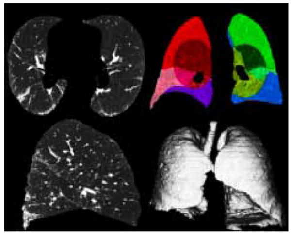
Lung Segmentation: 1st Row: Transverse slice, Coronal slice (Peripheral and Central Regions and Lobes Outlined by color); 2nd Row: Sagittal slice, Volumetric Rendering

2.1.2 Broncho-vascular Segmentation

One of the advantages of three dimensional data is that the broncho-vascular tree can be recognized and segmented. It is not possible to build a classifier that can successfully recognize tubular structures which may be arbitrarily sliced in a 2D HRCT image. Xu et. al. have shown significant classification improvement of emphysema by the 3D AMFM algorithm performed after broncho-vascular exclusion [15]. Lungs with UIP/IPF contain a lot of high-attenuating pathologies (fibrosis) compared to low-attenuating pathologies (emphysema). Thus segmentation of the vascular tree is more challenging than segmentation of the bronchial tree.

Segmentation of the trachea and its central bronchial branches is performed by an iterative process of 6 or 8 neighbor region growing algorithm thresholded at different levels to optimally extract as much of the tracheobronchial tree as possible, but prevent inclusion of erroneous low-attenuating pathologies (such as emphysema) by limiting the number of connected components from the seed point by a method similar to Aykac et al. [21].

Segmentation of the pulmonary vasculature is a challenging problem still under investigation. When trying to estimate high-attenuating pathologies like fibrosis and honeycombing it is important to account for other high-attenuating normal structures like vessels to lower the rate of false positive errors. Algorithms have tried to account for various common cross-sections of vessels that may appear in a 2D HRCT [22].

All 2D algorithms suffer from high false positive errors for identification of vessels in the presence of abnormal high-density lung tissues, such as those seen with UIP/IPF, due to the similarity of density between blood and the fibrotic lung. Several methods have been proposed to segment vessels in normal lungs where the vessels are the main high-attenuating tissue in the lungs [23]. Segmentation of the pulmonary vasculature in lungs with more than mild high-attenuating diffuse pathologies has not been addressed. Major morphological changes occur in lungs with UIP/IPF. The increased fibrotic pathologies result in the lung volume shrinking including significant distortion of the vessels and airways within those regions. Our histogram signature classification method of parenchymal classification does not require segmentation of the vessels and airway in these regions, however, it is useful for reduction of false positive classification to extract normal broncho-vascular structures in parts of the lung where severe architectural distortion has not occurred. Thus it was our goal to perform a semi-automatic segmentation of the vessels roughly greater than one third of the VOI. For a 15×15×15 pixel VOI at 0.625mm³ resolution, vessels approximately 3mm in diameter (up to the 5th generation) or larger were segmented. This was performed by filtering the dataset with a 3D line enhancement filter (sigma = 2) which is based on the examination of the eigenvalues of the Hessian matrix [24]. The Hessian matrix is composed of the partial second derivatives of the image and describes the second order structure of the intensity values surrounding each point in the image. The filtered image was then thresholded at a value determined specifically for the dataset by an expert, to include as much vasculature as possible with the least amount high-attenuating pathology. Figure 2 depicts a broncho-vascular segmentation from one of the datasets.

Fig. 2.

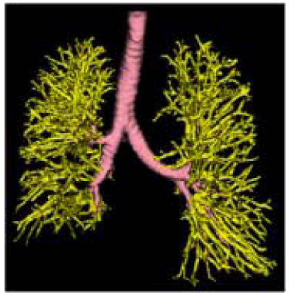
Broncho-vascular Structure. The Bronchial tree (pink) was segmented using an algorithm involving morphological operations and region growing [21]. The Vascular tree (yellow) was segmented by thresholding the 3D line enhancement filtered image [24].

2.2 Adaptive Binning of the histogram

A histogram is a discrete function which bins the voxels in a volume based on their intensity [25]. The location and width of each bin and the spacing between bins are the histogram parameters. Standard histogram analysis in CT involves equidistant spacing between the histogram bins. Adaptive binning enables the distance between the bins to be determined by the image data.

Adaptive binning can be accomplished using a K-means clustering algorithm. Clustering algorithms have the potential to more accurately describe the distribution of the histogram. However, the integrity of the clustering depends on the particulars of the algorithm. The standard iterative algorithm is initialized by a random selection of centroids. An iterative operation follows in which the distance from a point to each centroid is computed. The point is assigned to the cluster with the nearest centroid, and the cluster's centroid is updated. This iterative process continues for each point until a stopping criteria is met. Possible stopping criteria include reaching the maximum number of clusters or no change in cluster centroids between iterations. Other versions of K-means clustering iteratively compute the variance of the clusters as well. For these algorithms, varying stopping criteria are used [26]. The advantages of K-means clustering algorithms include easy implementation and relatively fast execution for a small sample size. The disadvantages of iterative K-means algorithms are that they are dependent on the initialization points so they may succumb to a less than optimal clustering by entrapment in a local minima. It is possible to compute an optimal K-means clustering of a histogram through recursion. A fast recursive algorithm can be implemented by using dynamic programming [27].

Dynamic programming is an effective algorithm design technique for approaching recursive problems [28]. Recursive problems are first initialized, and subsequent computations are formulated so that they depend on the previous computation. Systematically storing previous computations minimizes the current computation.

Define C[n] [k] as the minimum possible cost over all clusters of the histogram of length n into K clusters, where the cost of each cluster partition is the minimum within-class variance. Thus defined this function can be evaluated:

$$C[i][k]=\underset{\begin{array}{l}1\le i\le n,\\ 1\le j\le i\end{array}}{\text{min}}\{C[i][k-1],C[j][k-1]+I[j+1][i]\}$$ (1)

where, C[i] [k − 1] is the minimum cost of splitting the histogram bins 0 to i into k − 1 clusters; similarly C[j] [k − 1] represents the minimum cost of splitting the histogram bins 0 to j into k − 1 bins which is added to the cost of binning histogram bins j + 1 to i together.

2.3 Signatures and the Canonical Signatures

A histogram signature is made up of a histogram that has been clustered into K clusters, and is defined as follows,

$$\text{Sig}=\{({\mu }_1,w_1),\dots ,({\mu }_i,w_i),\dots ,({\mu }_K,w_K)\}$$

where μ_i is the centroid of the cluster and w_i is the weight of the cluster (the number of voxels in the cluster). The canonical signature for a class is computed by combining the signatures for each of the training VOIs and re-clustering the distribution into K clusters. The creation of a canonical signature allows for a more computationally efficient way to match signatures instead of computing the distance between all training signatures and all test signatures. Each cluster centroid can be thought of as a texton, which is a cluster of intensity values representing some texture property as in [29,19]. Thus the signatures from each training image in each class are grouped or in other words, all the textons are grouped and reclustered. Figure 4 shows the accumulated signatures in the top plot and the canonical signature created from various amounts of training data used in the bottom plot. Notice that an optimal clustering is achieved irrespective of the amount of training data used. The reclustering of all of the training signatures using the adaptive binning algorithm presented in the previous section maintains the integrity of the signatures; specifically the centroid location, the intra-centroid distance, and the weight of the centroids. The clustering of the accumulated centroids results in a representative signature of K centroids. Figure 5 shows the representative canonical signatures computed in the development and testing of our algorithm for five classes.

Fig. 4.

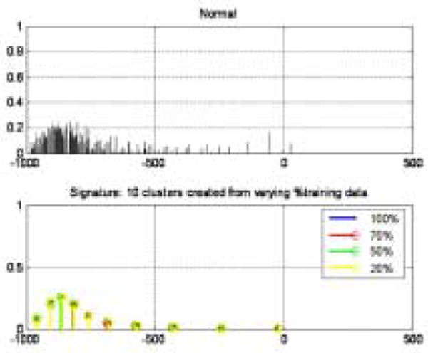
Creation of canonical signature. Top plot: Accumulated signatures from training set. Bottom plot: Canonical signatures computed by re-clustering the top plot using various amounts of training data.

Fig. 5.

The canonical signatures computed for each class (Normal, Reticular, Ground glass, Honeycombing, and Emphysema) are plotted in this figure. These signatures are made up of 4 cluster centers positioned at various locations with varying frequencies. Each signature is uniquely computed for each class.

2.4 Similarity Metrics

The earth mover's distance (EMD), first proposed by Rubner, is a cross-bin similarity metric which computes the minimal cost to transform one signature into another [18]. The EMD is modeled as a “transportation” problem and can be solved using efficient linear programming algorithms. Let P = {(μ_pl, w_pl),…, (μ_pm, w_pm)} be the first signature with m clusters and let Q = {(μ_q1, w_q1) ,…, (μ_qn,w_qn)} be the second signature with n clusters, where (μ, w) is a cluster and μ is the center of the bin and w is the number of voxels in the bin. Given two signatures with disparate bins, computing the EMD can be thought of as how much work does it take to transform signature P into signature Q. The clusters in P are thought of as the ‘supplies’ located at centroids μ_pi with the amount w_pi and the clusters in Q are thought of as the ‘demands’ located at centroids μ_qi with the amount w_qi. The EMD is the minimal amount of work required to transform P into Q. Let D = [d_ij] be the L₁ norm distance between μ_pi and μ_qj. Let F = [f_ij] be the ‘flow’ between μ_pi and μ_qj which minimizes the amount of work. The EMD is the minimum amount of work normalized by the total flow defined as

$$\begin{array}{l}\text{EMD}(\text{P},\text{Q},\text{F})=\frac{{\sum }_{i=1}^m{\sum }_{j=1}^n{d}_{\text{ij}}{f}_{\text{ij}}}{{\sum }_{i=1}^m{\sum }_{j=1}^n{f}_{\text{ij}}}\\ \text{such that},{\sum }_j{f}_{\text{ij}}\le p_i,\\ {\sum }_i{f}_{\text{ij}}\le q_j,\\ {\sum }_{i,j}{f}_{\text{ij}}=\text{min}\left\{{\sum }_i{p}_i,{\sum }_j{q}_j\right\},\\ \text{and}{f}_{\text{ij}}\ge 0\end{array}$$ (2)

The EMD has been shown to match perceptual distance better than other metrics [18]. The EMD is well suited to medical image analysis given the amount of intra-class variation which exists as a result of varying grades of pathology, uniqueness of each patient, inflation of the lungs, and scanner and scanning parameter differences.

The EMD is an exact metric when applied to probability distributions. It has been shown that the EMD is equivalent to the statistically based Mallows distance for probability distributions [30].

2.5 Experimental Evaluation

This section presents in detail the methods of how we tested our algorithm. The first section describes the data we used. The second section describes the creation of the training VOI database. The third section describes the creation of the testing dataset. The fourth and fifth section present the performance metrics we used to analyze our algorithm on the training and testing dataset respectively.

2.5.1 Data

Patients with moderate UIP/IPF were scanned for clinical purposes on a Lightspeed 8-detector GE Medical Systems CT scanner in helical mode with 8 × 1.25 mm detector configuration at a pitch of 1.35 utilizing 140kVp and approximately 250mAs. Images were reconstructed with 1.25mm slice thickness in a high-frequency sparing algorithm (BONE) with 50% overlap and a 512 × 512 axial matrix, producing approximately 0.625 mm³ isotropic voxels. Eighteen scans were used in this study. Fourteen datasets were used to create the training dataset upon which the canonical signatures were developed and the remaining four datasets were used to test the algorithm on new unseen data.

2.5.2 Training Set: Independent Volumes of Interest

Analyze and AVW were used to create a database containing independent cubic samples of various classes. Experts were asked to outline regions containing greater than 70% of the following classes: Normal, Honeycombing, Reticular, Ground glass, and Emphysema. The traced regions were stored as object maps which could then be further manipulated. Object maps efficiently map and store delineated regions. Traced regions for fourteen datasets were collected as object maps. The object maps were fed through an AVW program which extracts cubic volumes of interest (VOIs) of a pre-defined dimension. The VOI was defined empirically to be 15×15×15 cubic voxels. These VOIs are efficiently stored in a database along with which dataset they came from, their location in the lung, and their class label. Figure 6 shows the cubic VOIs selected within the expert drawn regions. Figure 3 shows a cubic VOI for the five classes that were labeled by the experts: Honeycombing, Reticular, Ground glass, Normal, and Emphysema. The training set used was composed of 15×15×15 cubic voxel VOIs of the following: Honeycombing (# of VOIs 337), Reticular (130), Ground glass (148), Normal (240), and Emphysema (54).

Fig. 6.

Independent Volumes of Interest (VOI): transverse, coronal, sagittal Views of cubic VOIs selected within expert drawn regions. The colored cubes represent different VOIs selected within the manually traced region (red) by the expert for this particular dataset.

Fig. 3.

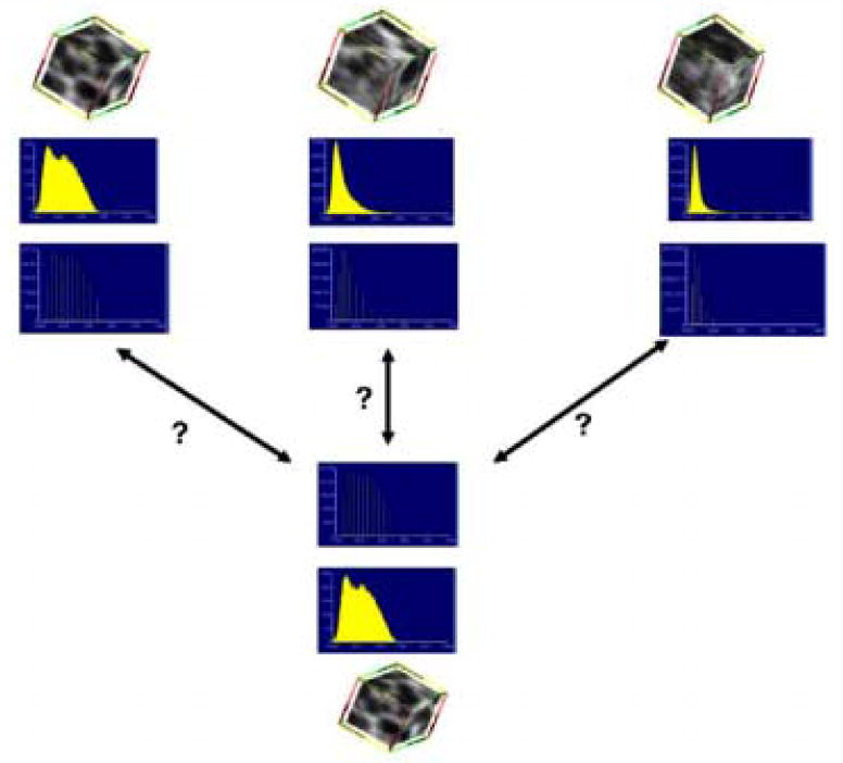
The main point of the algorithm is detailed in this figure. The top three rows show the cubes of data that are known along with their histograms and canonical signatures. The bottom three rows show an unknown cube of data with its histogram and signature. The idea of the algorithm is to compare the unknown signature with the known signatures using the EMD as the metric. The unknown cube of data is assigned to the known cube's class for which the signatures are most similar.

2.5.3 Testing Set: Whole lung Datasets

Experts were asked to manually segment complete lung datasets. Three experts each manually segmented four complete datasets. The experts labeled regions as Normal, Reticular, and Honeycombing. The four datasets manually segmented did not contain Ground glass or Emphysema tissue classes. Object maps for each segmentation were created. The Broncho-vascular object maps were added to the expert object maps to create a complete segmentation. Figure 7 shows the manual segmentation of one of the four datasets by three Experts; Expert 1: column 1, Expert 2: column 2, Expert 3: column 3.

Fig. 7.

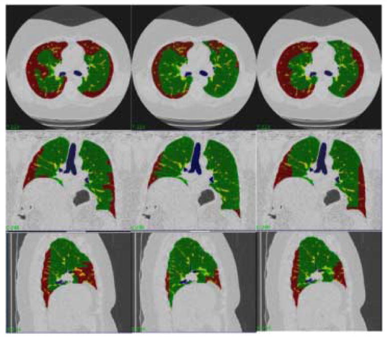
Each column is a segmentation of a dataset by a different expert. Each row is a different orientation (transverse, coronal, and sagittal). The colors represent different tissue classes: Green-Normal and Red-Reticular.

2.5.4 Performance Measures for Analysis of Classification of Independent Volumes of Interest

We used three performance measures to analyze the results of the classifier. If we have N classes, then define the set of known classes as C = {C₁,…, C_N} with |C_i| as the total number of samples in class C_i and the set of labeled classes as L = {L₁, …, L_N} with |L_i| as the total number of samples labeled as L_i.

Confusion Matrix

The confusion matrix is a K × K matrix where the rows represent L and the columns represent C. The diagonal of the confusion matrix represents the correctly classified VOIs.

Sensitivity and Specificity

Sensitivity or the true positive rate, is the proportion of each class where the expert and classifier agreed disease was present. Specificity or the true negative rate, is the proportion of each class where the expert and classifier agreed disease was not present. Sensitivity and specificity for class i were defined as follows,

$$\begin{array}{l}{\text{Sensitivity}}_i=\frac{\left|L_i\right|}{\left|C_i\right|}\\ {\text{Specificity}}_i=\frac{\left|L_j\right|}{\left|C_j\right|},\text{where}j=1,..,N\text{and}j\ne i\end{array}$$

Error Rate

The error rate is the number of misclassified samples.

$$\text{Error}=\text{∑}_{i=1}^N\text{∑}_{\begin{array}{l}j=1\\ j\ne i\end{array}}^N\frac{\left|L_i\right|}{\left|C_j\right|}$$

Each performance metric was validated over a 10-fold stratified cross validation. A N-fold stratified cross validation splits the data randomly into N partitions. Each partition contains the same proportion of each class as the complete dataset. The classification is performed N times, each time using N-1 of the partitions as the training set and using the one left out as the testing set. The N performance measures are averaged over the N = 10 folds. The training of the final classifier uses all of the available data and it's error rate is estimated as the average of all N=10 error estimates.

2.5.5 Performance Measures for Analysis of Classification of Test Lungs

The entire lung is classified and is compared to the three expert manual segmentations. The Jaccard Similarity Coefficient and the Volume similarity metric are used as metrics to measure level of agreement. The Jaccard Similarity Coefficient (JC) is defined as:

$$\text{JC}=\frac{X\cap Y}{X\cup Y}$$

JC measures the degree of overlap between two sets X and Y. It is zero when the two sets are disjoint and one when the two sets are totally overlapped. The Volume similarity metric (VS) is defined as:

$$\text{VS}=1-\frac{\left|\right|X|-|Y\left|\right|}{\left|X\right|+\left|Y\right|}$$

VS measures the degree of similarity in the volume of two sets, irrespective of the spatial location of the elements in the set. It is zero when the two sets are disjoint and one when the two sets have equal volumes.

The Williams Index

The Williams Index was first proposed by Williams [31] as a statistical measure of agreement between raters. The Williams Index measures how well an isolated rater agrees with the group of raters. It has since been used in medical image processing where no ground truth exists and algorithms must be compared to various experts as in comparing the result of a boundary detection algorithm to several manually drawn boundaries by experts [32]; it has also been used to compare the results of various classifiers when no ground truth is present [33]. The Williams Index is a ratio of the agreement of rater j to the group versus the overall group agreement and is defined mathematically as follows

$${\text{WI}}_j=\left(\frac{n-2}{2}\right)\frac{\text{∑}_{j\prime =\text{1},j\prime \ne j}^{n}a(D_j,D_{j\prime })}{\text{∑}_{j\text{'}=\text{1},j\text{'}\ne j}^{n-1}\text{∑}_{j">j\text{'}}^{n}a(D_{j\text{'}},D_{j^{″}})}$$

where a(D_j, D_j′) is a measure of similarity or agreement between raters j and j′. We used two similarity measurements: Jaccard Similarity Coefficient and the Volume Similarity Metric defined above [33]. If the confidence interval (CI) of the Williams Index for rater j includes 1, then it can be said that rater j agrees with the group as well as the members of the group agree with themselves. If the numerator and the denominator differ at the 100α percent level then the CI will not contain one.

3 Results

We present the results of our experimental methods in two sections. The first section presents the results of the development of our classifier on the training dataset of individual VOIs. Results on the following experiments are presented: 2 class, 4 class, and 5 class. The second section presents the results of the classifier on the testing of whole lung datasets and how the algorithm compares to the experts. Additionally, the quantification of lung tissues by the algorithm is compared to the experts' quantification of lung tissues.

3.1 Independent Volumes of Interest

The following results were obtained by performing a 10-fold stratified cross-validation on the dataset of independent VOIs described previously.

In order to determine the optimal number of clusters in a signature for a two class problem (Normal vs Abnormal) an ROC analysis was performed. The sensitivity and specificity was measured as the number of clusters in the signatures varied. The optimal area under the curve (A_z = 0.9307) was attained with a sensitivity (true positive rate) of 92.96% and specificity (true negative rate) of 93.78% with an optimal signature size of 4 clusters.

The error rate for a multi-class problem (Normal, Reticular, Ground glass, Honeycombing, Emphysema) versus signature size is shown in Figure 8(a).

Fig. 8.

In order to determine the optimal number of clusters in a signature for a multi-class problem the error rate was measured as the number of clusters in the signature was varied. Figure (a), shows the least error with a 4 cluster signature. Figure (b), shows the sensitivity (true positive rate) in green and specificity (true negative rate) in yellow for the 4-class classification experiment of normal (N), reticular (R), honeycombing (H), and emphysema (E). Figure c, shows the sensitivity (true positive rate) in green and specificity (true negative rate) in yellow for the 5-class classification experiment of normal (N), ground glass (G), reticular (R), honeycombing (H), and emphysema (E). Note that the sensitivity for honeycombing class remains about the same for the 4 and 5 class problem. However, note that the sensitivity of the reticular class is significantly reduced in the 5 class problem - this is because of the similarity between the ground glass and reticular classes, detailed in the confusion matrices in Table 1 and Table 2

The confusion matrix for a four class (Normal, Reticular, Honeycombing, Emphysema) problem is shown in Table 1. The sensitivity and specificity for the four classes are shown in Figure 8(b). The confusion matrix for a five class (Normal, Reticular, Ground glass, Honeycombing, Emphysema) problem is shown in Table 2. The sensitivity and specificity for the five classes are shown in Figure 8(c).

Table 1.

4 Class Confusion Matrix; Actual Class (rows) versus Classified Class (columns)

	Normal	Reticular	Honeycmbg.	Emphysema
Normal	201	12	10	3
Reticular	6	109	66	0
Honeycmbg.	1	6	221	0
Emphysema	9	0	2	42

Table 2.

5 Class Confusion Matrix; Actual Class (rows) versus Classified Class (columns)

	Normal	Reticular	Groundglass	Honeycmbg.	Emphysema
Normal	201	8	12	10	3
Reticular	5	26	14	35	0
Groundglass	1	44	95	31	0
Honeycmbg.	1	39	6	221	0
Emphysema	9	0	0	2	42

3.2 Whole Lung Datasets

The William's Index (WI) for the algorithm and the three experts for each label are shown in Figure 9. The 95% (Z = 1.96) confidence interval (CI) was computed. If 1 falls within the CI then we can conclude that the rater j agrees with the rater j′ as much as j′ agrees with the rest of the raters. Figure 9(a) shows the CI of the WI computed using the Jaccard Coefficient. Figure 9(b) shows the CI of the WI computed using the Volume Similarity Metric.

Fig. 9.

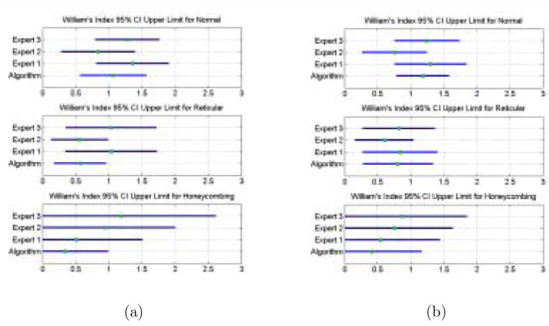
The Williams Index CI for the Algorithm and the Experts for each class computed using the Jaccard Coefficient shown in (a). and the Volume Similarity Metric shown in (b). The Williams index tests the ability of an isolated rater to agree with the group as much as the members of the group agree amongst themselves. An upper limit of the confidence interval greater than or equal to one is indicative agreement. The metric used to measure agreement makes a difference.

The average Jaccard Coefficients for the algorithm versus experts (AE) and for the experts versus experts (EE) are shown in Table 3. The results of a univariate T-test performed for each of the four classes to determine a difference in the means of the JC overlap between AE and EE are also listed in Table 3. A multivariate test comparing the difference of AE to EE given all four classes was also performed using the Hotelling T² statistic. The results of this analysis are a T² = 26.15 and a F = 8.15 with degrees of freedoms 3 and 29, and a p-value of p = 0.0004, also listed in Table 4.

Table 3.

Differences in Jaccard Overlap between the average Algorithm/Expert overlaps and the Expert/Expert overlaps for each class individually; the H₀ hypothesis is μ₁ – μ₂ = 0

	AE		EE		t (62 dof)	p
	μAE,	σAE	μEE,	σEE
Normal	0.60,	0.27	0.68,	0.26	-1.20	0.230
Reticular	0.18,	0.17	0.24,	0.21	-1.44	0.155
Honeycmbg.	0.02,	0.06	0.19,	0.30	-3.15	0.003
Emphysema	0	0	0	0	-	-

Table 4.

Hotelling T² multivariate test comparing the AE to EE given all four classes.

T2 (3 dof)	F (29 dof)	p
26.15	8.15	0.0004

A three dimensional rendering of a completely classified lung dataset as it is rotated around the Z axis is shown in Figure 11. Figure 12 shows the amount of each tissue type in the lungs classified by the algorithm and the three experts for each of the four datasets. The volume values were put into a 4×4 matrix where the classes are the rows and raters are the columns. An intra-class correlation measure and an analysis of variance were performed to measure the degree of similarity of volume classification between the algorithm and the three experts. The ICC is a metric which approaches 1 if the values in each row of the matrix are similar. The analysis of variance F statistic is greater than 1 if a significant difference exists. The results are as follows: Dataset 1: ICC = 0.9984, F = 0.0007; Dataset 2: ICC = 0.9559, F = 0; Dataset 3: ICC = 0.8623, F= 0.0015; Dataset 4: ICC = 0.7807, F = 0.0136.

Fig. 11.

Volumetric rendering of a classified lung. Purple is Normal, Red is Reticular, Green is Honeycombing, Yellow is Vessel, and Blue is Airway

Fig. 12.

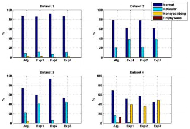
Lung Volumes calculated by Algorithm and Experts. Dataset 1, ICC = 0.9984; Dataset 2, ICC = 0.9559; Dataset 3, ICC = 0.8623; Dataset 4, ICC = 0.7807

4 Discussion

Although the microscopic changes in UIP/IPF are below the resolution of traditional CT imaging, near microscopic changes in attenuation and gross parenchymal distortion resulting from idiopathic pulmonary fibrosis can be visualized on HRCT. The visual changes include varying types of high-attenuating pathology, distortion of normal broncho-vascular structures and areas of end-stage fibrosis, including regions characterized visually on HRCT as ground glass infiltrates, coarse reticular infiltrates, regional traction bronchiecstasis and honeycombing. Our purpose in developing an algorithm to detect these features associated with pulmonary fibrosis is to characterize and reproducibly quantify the extent of pulmonary involvement by UIP/IPF. The first task in developing a CAD algorithm to aid in the quantification and classification of pathology is to distinguish between normal and abnormal tissue. When cluster-type methods are used, one of the optimal parameters that must be tested is number of clusters. We performed an ROC analysis varying the size of the signature (number of clusters) and determined that a signature containing 4 clusters was most discriminatory. The area under the curve was computed, A_z = 93.07, which is the average sensitivity over all specificities [34]. We have shown that our method can distinguish between normal and abnormal three dimensional volumes of interest with a sensitivity of 92.96% and specificity of 93.78%.

Our second objective was to test the classifier's ability to distinguish between various types of high-attenuating pathologies. This is a considerably more challenging task because of the continuous evolution of the disease leading to a high intra-class variation and to fuzzy distinctions between grades and types of pathology. The class types are:

• Normal: slightly more dense than air, tissue contains small bronchioles and vessels

• Ground glass: increased homogeneous opacity of pulmonary parenchyma where normal broncho-vascular structures remain apparent - this is a non-specific finding that may represent many pathologic changes including microscopic fine fibrosis, interstitial cellular infiltration, increased parenchymal water or tissue compression

• Reticular: abnormal irregular linear parenchymal opacities that may represent near-microscopic parenchymal fibrosis

• Honeycombing: moderately thin-walled, air-filled cysts that do not communicate with airways, corresponding to regions of end-stage dense fibrosis and architectural distortion; variable sizes from microscopic to several millimeters

• Emphysema: Regions of pulmonary parenchymal destruction resulting in large air-filled spaces or decreased attenuation of the parenchyma due to microscopic changes not directly apparent on HRCT

The ability of a classifier to distinguish between Ground glass, Reticular, and Honeycombing and their grades depends on how it is trained. The traditional method of choosing defined box regions which contain at least 70% of the tissue class introduces errors in the training of the classifier. Our classifier was trained with a high intra-class variation for every class by using fourteen datasets to construct our training database.

Again, because we are using cluster-type methods, we tested for the optimal signature size given a multi-class problem. The error rate for various signature sizes using a 10-fold stratified cross validation method was computed. As can be seen in Figure 8(a) the signature containing 4 clusters was again most discriminatory. To test our second task two tests were performed, first a four class problem, and second a five class problem.

The four class problem included the following classes: Normal, Reticular, Honeycombing, and Emphysema; The classifier sensitivity and specificity for the Reticular and Honeycombing pathologies is less than that of Normal and Emphysema, see Figure 8(b). Table 1 shows the misclassification between Honeycombing and Reticular. This decreased sensitivity and specificity is in part a result of high intra-class variation but primarily due to the inherent gradations of the microscopic pathology and resultant incomplete separation of the visual appearance of these findings in these areas. Specifically, this is exem-plified at the Reticular/Honeycombing boundary where visually the Reticular class contains severely course linear abnormalities that appear almost cystic and the Honeycombing class contains only barely apparent small cysts with a large amount of adjacent increased opacity that is presumably fibrosis.

The five class problem included the following classes: Normal, Ground glass, Reticular, Honeycombing, and Emphysema; This problem tackles the very challenging distinction between Ground glass and Reticular pathologies present in lungs with mild to moderate UIP/IPF. The sensitivity and specificity for Ground glass, Reticular and Honeycombing is decreased, as seen in Figure 8(c). As expected, since the visual appearance is most similar, the Reticular class which includes grades of pathology in between Ground glass and Honeycombing is most decreased. Table 2 shows the Reticular class as most misclassified, with either Ground glass or Honeycombing. Again, the decreased sensitivity and specificity are a result of high intra-class variation and the gradual contiguity of visual and pathologic changes in the parenchyma which result in no-distinct appearance in many regions this probably represents mixed or transitional microscopic involvement. However, even though there may be some misclassification or decreased discrimination between similar abnormalities for our classifiers, it is more important that the methods provide a consistent result that agrees with the experts as frequently as the experts agree among themselves, particularly in a setting were an objectively defined gold standard outside of the expert opinion does not exist.

Medical image processing validation often can not rely on availability of true gold standards. Gold standards based on experts' interpretation or correlation with other imaging modalities and/or with pathology have been developed [35]. The comparison of a manual segmentation to a computer algorithm's classification is another issue. The resolution at which a computer algorithm can classify pathology is much finer than a manual segmentation can typically accomplish, especially for diffuse lung pathology. Hence, standard measures of overlap are less than optimal because of the varying resolutions of the regions, so we use a volume similarity metric as well. Lacking a gold standard we used the William's Index to measure our algorithm agreement with the experts as well as the experts agreement with themselves. A William's Index with an upper confidence interval greater than 1 would affirm our claim. Figure 9(a) shows that when the Jaccard Coefficient is used as the metric of agreement, the algorithm agrees with the experts for the definition of Normal class yet it does not quite agree as well with the definition of Reticular and Honey-combing. On the other hand, Figure 9(b) results in the upper limit of the CI greater than one for the Algorithm in every class. Additionally, because the CI's for the Algorithm and the Experts overlap it can be concluded that they are not significantly different from each other. Experts exhibit high inter-rater variability as a result of the very high intra-class variation and gradual evolution of pathology, making validation of a CAD algorithm problematical using experts as gold standards.

We also tested the agreement between the algorithm and the experts using the Jaccard Coefficient (JC), which is essentially a measure of overlap. The average overlaps (JC) and their standard deviations for the Algorithm versus Expert (AE) and for the Expert versus the Expert (EE) are shown in Table 3. When the results of the three classes are considered together, a significant difference exists between AE and EE with a Hotelling T² statistic of 26.15 and an F statistic of 8.15. A closer look at the difference in overlaps of AE and EE for each class individually helps to explain why there exists an overall difference between AE and EE. The T-statistic and the p-value for each test are listed in Table 3. No significant difference between AE and EE exists for Normal and Reticular class. However, for the Honeycombing class, the AE and EE are significantly different. Further investigation is needed to identify the reason for this discrepancy. The high intra-class variability as a result of the disease process is evident in the JC values below 50% for the Reticular and Honeycombing class by the experts (EE).

Regional quantification is one of the important goals for developing CAD algorithms on MDCT scans of lungs. Figure 11 depicts the regional localization of the disease made possible with this type of analysis. Figure 12 shows the amount of each tissue type in the lungs classified by the algorithm and the three experts for each of the four datasets, and Figure 10 shows a transverse slice of each of the four datasets. Notice the degree of inter-expert variation in Figure 10. The Algorithm and Experts agree best for Dataset 1 and 2. Note in Figure 10 row 2, column 2, in the lower central region of the right lung that the Algorithm has misclassified as Honeycombing a region of overlapping bronchioles and vessels. The algorithm found Honeycombing in dataset 3 where the Experts did not. This could be due to over classification by the Algorithm or a miss by the Experts. In this case, after review of the classification results by experts, it appears that the Algorithm labeled as Honeycombing a very course, dense Reticular pathology with some traction bronchiecstasis. The misclassification of traction bronchiecstasis (low density tube with adjacent fibrosis) for Honeycombing (low density cyst with adjacent fibrosis) is a result of classification of a small VOI which does not cover the extent of the tube nor account for circularity of the structure being classified. The Algorithm and the Experts disagreed most in Dataset 4. This Dataset contained a significant amount of large Honeycombing cysts that were at times larger than the 15×15×15 VOI. This resulted in classifying this region of large filled cysts as Emphysema and Reticular. Figure 10 row 4, column 2, shows the misclassification of Honeycombing tissue for Reticular and Normal. In addition to increasing the size of VOI, the inclusion of a wider range of Honeycombing type patterns in the training set would minimize this type of misclassification. Additionally, the subdivision of the Honeycombing class into large cysts versus small cysts, and into dense network of cysts versus isolated cysts, is necessary.

Fig. 10.

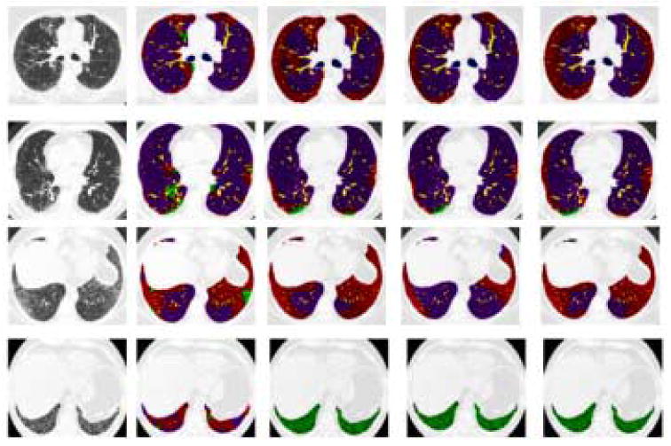
Classified Lungs by Algorithm and Experts. Rows 1-4 depict a transverse slice of Datasets 1-4. Column 1 is the original slice, Column 2 is the Algorithm's classification and Columns 3-5 are the Experts' 1-3 segmentation. Purple is Normal, Red is Reticular, Green is Honeycombing, Yellow is Vessel, and Blue is Airway

5 Conclusion

In conclusion this paper presents a novel method to texture analysis in the classification and quantification of pathology in 3D CT images. The method is computationally efficient and produces results comparable to expert radiologic judgment. Currently, the computation of signatures for a whole lung dataset can be performed in approximately ten minutes on a standard workstation with unoptimized code. We have demonstrated its effectiveness in the classification of normal versus abnormal tissue. Additionally, we have demonstrated that it performs as well as the experts in distinguishing between the pathologies present in lungs with UIP/IPF. We have summarized the challenges in validating a CAD algorithm on detection of diffuse lung pathologies from high-resolution MDCT data. The development of quantitative metrics in medical image processing will allow for the quantification of disease and thus, for objective measures of disease progression.

Specifically, in the case of UIP/IPF, the extent and visual features of this disease visually apparent on chest CT have been shown to be independent prognostic indicators. In combination with clinical and physiologic parameters, a clinical/radiological/physiologic score (CRP score) has been utilized to stage patients with this disease and predict its temporal course, which is typically progressive and leads to death within 5 years of diagnosis [36,37]. Since the CT radiologic findings are strong independent indicators of disease, it is critical to have accurate and reproducible quantification of the extent of disease. As an objective measure, our quantitative methods appear to provide such a capability and thus offer a means for accurately assessing and monitoring the disease progression and/or response to therapy.

References

- 1.Beigelman-Aubry C, Hill C, Guibal A, Savatovsky J, Grenier PA. Multi-Detector row CT and postprocessing techniques in the assessment of diffuse lung disease. Radiographics. 2005;25(6):1639–1652. doi: 10.1148/rg.256055037. [DOI] [PubMed] [Google Scholar]
- 2.Sutton RN, Hall EL. Texture measures for automatic classification of pulmonary disease. IEEE Transactions on Computers. 1972;21(7):667–676. [Google Scholar]
- 3.Kruger RP, Thompson WB, Turner AF. Computer diagnosis of pneumoconiosis. IEEE Transactions on Systems, Man, and Cybernetics. 1974;4:40–49. [Google Scholar]
- 4.Hall EL, William J, Crawford O, Roberts RE. Computer classification of pneumoconiosis from radiographs of coal workers. IEEE Transactions on Biomedical Engineering. 1975;22(6):518–527. doi: 10.1109/tbme.1975.324475. [DOI] [PubMed] [Google Scholar]
- 5.Turner AF, Kruger RP, Thompson WB. Automated computer screening of chest radiographs for pneumoconiosis. Investigative Radiology. 1976;11(4):258–266. doi: 10.1097/00004424-197607000-00002. [DOI] [PubMed] [Google Scholar]
- 6.Tully RJ, Conners RW, Harlow CA, Lodwick GS. Towards computer analysis of pulmonary infiltrites. Investigative Radiology. 1978;13:298–305. doi: 10.1097/00004424-197807000-00005. [DOI] [PubMed] [Google Scholar]
- 7.van Ginneken B, ter Haar Romeny BM, Viergever MA. Computer-aided diagnosis in chest radiography: A survey. IEEE Transactions on Medical Imaging. 2001;20(12):1228–1241. doi: 10.1109/42.974918. [DOI] [PubMed] [Google Scholar]
- 8.Gilman MJ, Richard J, Laurens G, Somogyi JW, Honig EG. CT attenuation values of lung density in sarcoidosis. Journal of Computer Assisted Tomography. 1983;7(3):407–410. doi: 10.1097/00004728-198306000-00003. [DOI] [PubMed] [Google Scholar]
- 9.Müller NL, Staples CA, Miller RR, Abboud RT. Density mask: An objective method to quantitate emphysema using computed tomography. Chest. 1988;94(4):782–787. doi: 10.1378/chest.94.4.782. [DOI] [PubMed] [Google Scholar]
- 10.Rienmüller RK, Behr J, Kalender WA, Schatzl M, Altmann I, Merin M, Beinert T. Standardized quantitative high resolution CT in lung disease. Journal of Computer Assisted Tomography. 1991;15(5):742–749. doi: 10.1097/00004728-199109000-00003. [DOI] [PubMed] [Google Scholar]
- 11.Müller NL, Coxson H. Chronic obstructive pulmonary disease 4: Imaging the lungs in patients with chronic obstructive pulmonary disease. Thorax. 2002;57:982–985. doi: 10.1136/thorax.57.11.982. [DOI] [PMC free article] [PubMed] [Google Scholar]
- 12.Goris ML, Zhu HJ, Blankenberg F, Chan F, Robinson T. An automated approach to quantitative air trapping measurements in mild cystic fibrosis. Chest. 2003;123:1655–1663. doi: 10.1378/chest.123.5.1655. [DOI] [PubMed] [Google Scholar]
- 13.Hartley PG, Galvin JR, Hunninghake GW, Merchant JA, Yagla SJ, Speakman SB, Schwartz DA. High-resolution CT-derived measures of lung density are valid indexes of interstitial lung disease. Journal of Applied Physiology. 1994;76:271–277. doi: 10.1152/jappl.1994.76.1.271. [DOI] [PubMed] [Google Scholar]
- 14.Sluimer I, Schilham A, Prokop M, van Ginneken B. Computer analysis of computed tomography scans of the lung: A survey. IEEE Transactions on Medical Imaging. 2006;25(4):385–405. doi: 10.1109/TMI.2005.862753. [DOI] [PubMed] [Google Scholar]
- 15.Xu Y, McLennan G, Guo J, Hoffman EA. MDCT-Based 3-D texture classification of emphysema and early smoking related lung pathologies. IEEE Transactions on Medical Imaging. 2006;25(4):464–475. doi: 10.1109/TMI.2006.870889. [DOI] [PubMed] [Google Scholar]
- 16.Zaporozhan J, Ley S, Eberhardt R, Weinheimer O, Iliyushenkio S, Herth F, Kauczor HU. Paired inspiratory/expiratory volumetric thin-slice CT scan for emphysema analysis. Chest. 2005;128(5):3212–3220. doi: 10.1378/chest.128.5.3212. [DOI] [PubMed] [Google Scholar]
- 17.Mendonca PR, Padfield DR, Ross JC, Miller JV, Dutta S, Gautham SM. Quantification of emphysema severity by histogram analysis of CT scans. MICCAI. 2005;8(Pt 1):738–44. doi: 10.1007/11566465_91. [DOI] [PubMed] [Google Scholar]
- 18.Rubner Y, Tomasi C, Guibas LJ. The earth mover's distance as a metric for image retrieval. International Journal of Computer Vision. 2000;40(2):99–121. [Google Scholar]
- 19.Varma M, Zisserman A. A statistical approach to texture classification from single images. International Journal of Computer Vision. 2005;62(12):61–81. [Google Scholar]
- 20.Hu S, Hoffman E, Reinhardt J. Automatic lung segmentation for accurate quantitation of volumetric X-ray CT images. IEEE Transactions on Medical Imaging. 2001;20(6):490–498. doi: 10.1109/42.929615. [DOI] [PubMed] [Google Scholar]
- 21.Aykac D, Hoffman EA, McLennan G, Reinhardt JM. Segmentation and analysis of the human airway tree from 3d X-ray CT images. IEEE Transactions on Medical Imaging. 2003;22(8):940–950. doi: 10.1109/TMI.2003.815905. [DOI] [PubMed] [Google Scholar]
- 22.Delorme S, Keller-Reichenbecher MA, Zuna I, Schlegel W, Kaick GV. Usual interstitial pneumonia: quantitative assessment of high-resolution computed tomography findings by computer-assisted texture-based image analysis. Investigative Radiology. 1997;32(9):566–574. doi: 10.1097/00004424-199709000-00009. [DOI] [PubMed] [Google Scholar]
- 23.Hidenori S, Hoffman EA, Sonka M. Automated segmentation of pulmonary vascular tree from 3D CT images. Proc SPIE Medical Imaging. 2004;5369:107–116. [Google Scholar]
- 24.Sato Y, Nakajima S, Atsumi H, Koller T, Gerig G, Yoshida S, Kikinis R. 3D multi-scale line filter for segmentation and visualization of curvilinear structures in medical images. Conference on Computer Vision, Virtual Reality and Robotics in Medicine and Medical Robotics and Computer-Assisted Surgery. 1997:213–222. [Google Scholar]
- 25.Gonzalez RC, Woods RE, Eddins SL. Digital Image Processing Using Matlab. Pearson Prentice Hall; 2004. [Google Scholar]
- 26.Jain A, Murty M, Flynn P. Data clustering: A review. ACM Computing Surveys. 1999;31(3):264–323. [Google Scholar]
- 27.Knopps ZF, Maintz JBA, Viergever MA, Pluim JPW. Normalized mutual information based registration using K-means clustering based histogram binning. Proc SPIE Medical Imaging. 2003;5032:1072–1080. [Google Scholar]
- 28.Bellman R. Dynamic Programming. Princeton, NJ: Princeton Univ. Press; 1957. [Google Scholar]
- 29.Varma M, Zisserman A. Texture classification: are filter banks necessary. IEEE Computer Society Conference on Computer Vision and Pattern Recognition. 2003:691. [Google Scholar]
- 30.Levina E, Bickel P. The earth mover's distance is the Mallows distance: some insights from statistics. IEEE International Conference on Computer Vision. 2001 [Google Scholar]
- 31.Williams GW. Comparing the joint agreement of several raters with another rater. Biometrics. 1976;32:619–627. [PubMed] [Google Scholar]
- 32.Chalana V, Kim Y. A methodology for evaluation of boundary detection algorithms on medical images. IEEE Transactions on Medical Imaging. 1997;16(5):642–652. doi: 10.1109/42.640755. [DOI] [PubMed] [Google Scholar]
- 33.Martin-Fernandez M, Bouix S, Ungar L, McCarley RW, Shenton ME. Two methods for validating brain tissue classifiers. MICCAI. 2005;3749:515–522. doi: 10.1007/11566465_64. [DOI] [PMC free article] [PubMed] [Google Scholar]
- 34.Hanley JA, McNeil BJ. The meaning and use of the area under a receiver operating characteristic (ROC) curve. Radiology. 1982;143:29–36. doi: 10.1148/radiology.143.1.7063747. [DOI] [PubMed] [Google Scholar]
- 35.Warfield SK, Zou KH, Wells WM. Simultaneous truth and performance level estimation (STAPLE. IEEE Transactions in Medical Imaging. 2004;23(7):903–921. doi: 10.1109/TMI.2004.828354. [DOI] [PMC free article] [PubMed] [Google Scholar]
- 36.Talmadge J, King E, Tooze JA, Schwarz MI, Brown KR, Cherniack RM. Predicting survival in idiopathic pulmonary fibrosis. American Journal of Respiratory and Critical Care Medicine. 2001;164:1171–1181. doi: 10.1164/ajrccm.164.7.2003140. [DOI] [PubMed] [Google Scholar]
- 37.Wells AU, Desai SR, Rubens MB, Goh NSL, Cramer D, Nicholson AG, Colby TV, du Bois RM, Hansell DM. Idiopathic pulmonary fibrosis: A composite physiologic index derived from disease extent observed by computed tomography. American Journal of Respiratory and Critical Care Medicine. 2006;167:962–969. doi: 10.1164/rccm.2111053. [DOI] [PubMed] [Google Scholar]