Uses and misuses of progress curve analysis in enzyme kinetics

Abstract

Progress curve analysis is a convenient tool for the characterization of enzyme action: a single reaction mixture provides multiple experimental measured points for continuously varying amounts of substrates and products with exactly the same enzyme and modulator concentrations. The determination of kinetic parameters from the progress curves, however, requires complex mathematical evaluation of the time-course data. Some freely available programs (e.g. FITSIM, DYNAFIT) are widely applied to fit kinetic parameters to user-defined enzymatic mechanisms, but users often overlook the stringent requirements of the analytic procedures for appropriate design of the input experiments. Flaws in the experimental setup result in unreliable parameters with consequent misinterpretation of the biological phenomenon under study. The present commentary suggests some helpful mathematical tools to improve the analytic procedure in order to diagnose major errors in concept and design of kinetic experiments.

1. Introduction

Enzyme activity is characterized in terms of rates [1], but the experimental enzyme assays measure substrate or product concentrations and not directly rates. The derivation of reaction rates from the changing concentrations is always an approximation with implicit error, but it is widely used in the determination of kinetic parameters because of the simplicity of its mathematical description with differential rate equations. Thus, in the simplest case the scheme $E+S\underset{k_{-1}}{\overset{k_1}{\rightleftarrows }}ES\stackrel{k_2}{\to }E+P$ is assumed, where E is enzyme, S is its substrate, P is the measured product, k₁, k₂ and k_-1 are the respective reaction rate constants. With the quasi-steady-state assumption the differential rate equation for this scheme is

$$\frac{dP}{dt}=\frac{k_2.E.(S_0-P)}{K_M+S_0-P}$$ (1)

where the subscript 0 indicates the initial value of concentration, the $K_M=\frac{k_{-1}+k_2}{k_1}$ is the so called Michaelis constant [1]. If P is measured over time, typically a linear increase in P is approximated from the initial phase of the reaction to define the rate $\frac{dP}{dt}$ and using a range of S₀ a simple optimization procedure can identify the K_M and k₂ values in Eq.(1) [2]. This approach offers a simple mathematical evaluation at the expense of imprecision in the linear approximation, which necessarily is reflected in the statistical variability of the parameters [2]. This imprecision can be overcome, if the measured data from the full time course of the reaction (called progress curve) are used and instead of differentiating the experimental data the model equation is integrated. Even for the simplest case given above, however, the mathematical analysis of the progress curves is rather sophisticated. According to [3], following integration Eq.(1) gives

$$t=\frac{1}{k_2.E}P+\frac{K_M}{k_2.E}\ln \frac{S_0}{S_0-P}$$ (2)

The problem of using Eq.(2) for optimization stems from the fact that its inverse function P=P^M (t,K_M,k₂,S₀,E), in which t is the independent variable, has no analytical form for P and thus specially designed mathematical approaches should be used for the identification of the parameters K_M and k₂ [3]. In order to overcome the necessity for mechanism-specific mathematical procedures, versatile programs for progress curve analysis have been developed (FITSIM, DYNAFIT) [4,5], in which numerical integration simulates progress curves according to the user-defined mechanism and following multiple iterations of the model parameters the sum of the squared differences (SSD) between the points of the simulated and experimental curves is minimized. These programs, which are based on sound theoretical grounds, are highly flexible and convenient for various catalytic mechanisms and accordingly their application is tempting even for researchers with little experience in enzyme kinetics. Despite their simplicity the analytic procedures pose certain requirements concerning the experimental design and if these are overlooked the overall analysis can be seriously flawed. The present survey provides an example for misuse of the progress curve analysis and suggests some helpful tools to detect errors in the experimental setup of such kinetic work.

2. Relevance of the reaction rate constants optimized by progress curve analysis

In order to achieve versatility of the application, the available programs operate with reaction rate constants, e.g. in the scheme shown in the Introduction the values of k₁, k_-1 and k₂ are varied in the course of the optimization procedure. This is a sound approach, if the user is aware of the fact that these constants are operational tools in the iterations and the relevance of their optimized values requires expert evaluation, which depends on the concrete experimental setup. For instance, if the experiment does not provide any direct information on the changes of the ES intermediate concentrations (as it stands for the majority of kinetic measurements), the time course of P generation is not sufficient to identify the absolute values of the rate constants. A simple inspection of the catalytic scheme in the Introduction indicates that different ratios of the rate constants for the formation and decomposition of the ES complex can result in the same concentration of the complex with consequent identical time course of P formation, which is actually measured. Thus, following optimization of the rate constants the task of the expert should be to formulate the relevant constant ratios, to which the experimental setup is sensitive.

For illustration of the issue mentioned above we will take an example from the recent literature. Progress curve analysis is applied in a study on the interactions of various mutants of pancreatic secretory trypsin inhibitor and trypsin [6]. The authors of this report worked with the scheme shown in the Introduction and claim that they have identified the k₁, k_-1 and k₂ rate constants for trypsin in the absence of inhibitor (“The k₁, k_-1 and k₂ rate constants were fixed values, which were determined from separate progress curves generated in the absence of inhibitor”). Using these constant values, the authors combine the basic scheme with a reaction of reversible enzyme-inhibitor interaction and try to estimate the rate constants of this superimposed process.

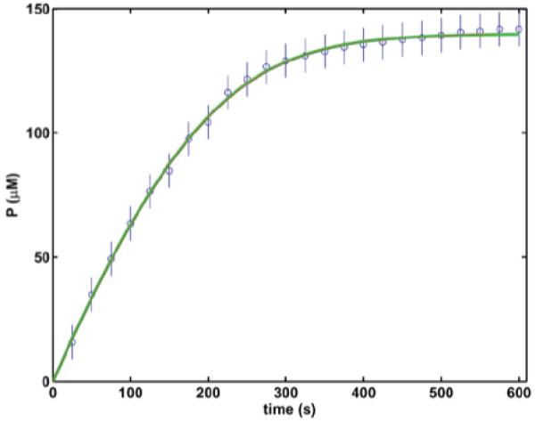
To further analyze the basic scheme, one can use the data of the control curve from Figure 4B of [6] as mean values of experimental progress curves (this is the control curve, in which the final product concentration approaches best the initial substrate concentration). Because the authors do not provide any information about the variance of their assay, one can assume that the deviation of the final P from the initial S in Figures 4A and 4C of [6] indicates the scale of the experimental uncertainties and accordingly we model the error of the experiment with flat standard deviation (SD) at each data point as shown in our Figure 1. Using numerical integration of the differential rate equations for the scheme $E+S\underset{k_{-1}}{\overset{k_1}{\rightleftarrows }}ES\stackrel{k_2}{\to }E+P$, progress curves are simulated with different rate coefficients k₁, k_-1 and k₂. Progress curves gained with three different sets of rate constants are shown in Figure 1. Although there is a six-order of magnitude difference in the k_-1 values (between 0.005 and 1000 s^-1) and an order of magnitude difference in the k₁ values (between 1.35 and 13.4 μM^-1.s^-1), the three simulated progress curves are indistinguishable by visual inspection. It is noteworthy that these three sets of rate constants were gained with the help of a SSD minimization procedure using the Nelder-Mead simplex direct search method [7], in which the optimization criterion was set at the level of 1 relative SD span for the mean normalized SSD (each member of the SSD was normalized by division with the modeled SD for the respective time point and the sum was divided by the number of time points). All three sets of fitted rate constants satisfy this criterion despite the significant differences in their values. Thus, neither the visual, nor the numeric inspection of the simulated processes can discriminate between multiple sets of rate constants, each of which satisfactorily describes the time course of the reaction. This example argues against the validity of the cited claims that the reaction rate constants have been determined and as a direct consequence their further application in enzyme-inhibitor assays is profoundly questionable.

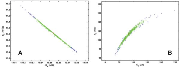
Figure 4.

Michaelis and catalytic constants estimated by Monte Carlo simulation of progress curves. The mean and SD values of P in Figure 1 are used to define the distribution of the source data. The Michaelis constant K_M and the catalytic constant k₂ are optimized as described in the text for Figure 2 in 1000 synthetic cycles. The initial values used in the optimization procedures are K_M=20 mM, k₂=14000 s^-1 for panel A and K_M=200 μM, k₂=200 s^-1 for panel B. The estimated synthetic parameters are shown by symbols in green (for pairs within the 95% minimal-volume region) or blue (for pairs out of this confidence region).

Figure 1.

Progress curve of trypsin catalyzed reaction analyzed by numerical fitting of reaction rate constants. The concentration of released p-nitroaniline in the course of action of 10 nM trypsin on 140 mM N-CBZ-Gly-Pro-Arg-p-nitroanilide substrate is shown as mean (symbols, values taken from the control curve of Fig. 4B of [6]) and SD (bars, values modeled from the final P in the three control curves in Fig. 4 of [6]). Lines represent simulated progress curves for P according to the scheme using the following combinations of reaction rate constants: green, k₁=1.42 μM^-1.s^-1, k_-1=6.78 s^-1, k₂=114 s^-1; red, k₁=1.35 μM^-1.s^-1, k_-1=0.005 s^-1, k₂=113 s^-1; grey, k₁=13.4 μM^-1.s^-1, k_-1=1000 s^-1, k₂=112 s^-1.

3. Relevance of the Michaelis constant optimized by progress curve analysis

If the expert re-evaluation of the optimized rate constants from Figure 1 is performed as discussed in the preceding section, the Michaelis constant $K_M=\frac{k_{-1}+k_2}{k_1}$ can be calculated from the three sets of parameters. The three combinations of rate constants used in Figure 1 yield remarkably similar K_M values: 85.06, 83.71 and 82.98 μM. Does this mean that if once all three rate constants cannot be defined, working with a single substrate concentration progress curve analysis still allows at least reliable determination of K_M and k₂? The answer is definitely ‘no’ in real experiments. The authors of FITSIM emphasize that ‘the number of varied parameters should be equal to, or less than, the number of experimental progress curves entered for correct convergence and well-determined final parameters to be obtained’ [4]. Other authors also warn against using a single time-course for determination of K_M and k₂ [8]. An alternative analysis of the data in Figure 1 supports these recommendations.

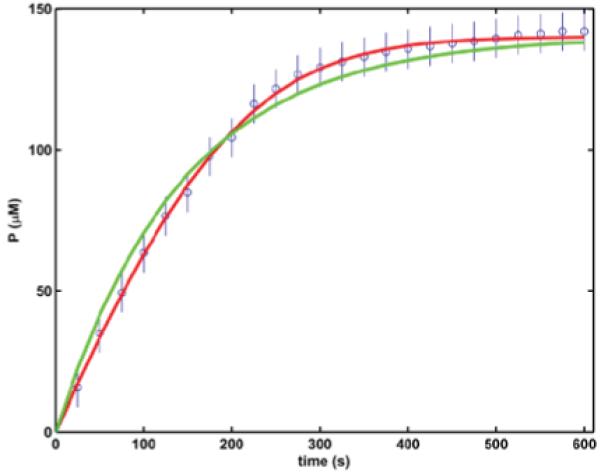
Instead of the rate constants, in the alternative analysis the K_M and k₂ are iterated using the integrated model Eq.(2) and our recently published optimization procedure [3]. As shown in Figure 2, at least two pairs of parameters meet the convergence criterion to simulate the progress curve with a normalized SSD less than 1. The difference in their values spans three orders of magnitude and there is no straightforward indicator for which pair is the better estimate. The lack of singularity stems from the poor experimental design: working with one starting substrate concentration it is very difficult (even impossible) to identify systematic uncertainties [9].

Figure 2.

Progress curve of trypsin catalyzed reaction analyzed by optimization of the Michaelis and the catalytic constants. The data are the same as in Figure 1, but the integrated equation

$$t=\frac{1}{k_2.E}P+\frac{K_M}{k_2.E}\ln \frac{S_0}{S_0-P}$$

is used for fitting the parameters K_M and k₂ as described in [3]. Lines represent simulated progress curves for P using the following combinations of parameters: red, K_M=84.4 μM, k₂=113.3 s^-1; green, K_M=19.9 mM, k₂=14020 s^-1.

4. Monte Carlo simulation as a diagnostic tool in progress curve analysis

When biological processes are formalized in mathematical terms, measured experimental data are used to derive model parameters as general characteristics of the process under study. A legitimate requirement in biological modeling is to provide not only the best estimate of the parameters, but also a statistical measure of their variability. However, even in the case of the simplest models the statistical distribution of the parameters can be described only with complicated and model-specific analytic weighting procedures for conversion of the uncertainties of the measurement into confidence intervals of the parameters. An alternative robust approach for determination of statistical variance of model parameters is the Monte Carlo simulation and its variants [10,11]. The principle of this approach is that the measured data define the distribution of the sampled quantity (e.g. product concentration in different points of the progress curve) and thereafter a computer performs a great number (1000-1500) of virtual experiments: it draws random samples from the modeled distribution of experimental data and estimates the synthetic model parameters on the basis of these quasi-experimental points. The synthetic sets of parameters are flipped around the original model parameters. The mean of the gained 1000-1500 points determines the best guess for the needed model parameters, whereas their distribution, which reflects the uncertainties of the experiment, determines their multidimensional “root” confidence intervals (for further details see [12,13]).

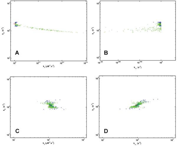
In addition to the typical application of Monte Carlo simulations described above, their inclusion as a routine supplement of progress curve analysis can be of special benefit for screening the adequateness of interpretation of the model parameters. For example, Monte Carlo simulation with the data and the optimization approach of Figure 1 would explicitly show that the experimental setup is not sensitive to the values of the three rate constants. Figure 3 illustrates that with these experimental data the fitting procedure to a model with three parameters converges successfully with ranges of k₁ and k_-1 values spanning orders of magnitude. Using two different sets of initial parameter values, the difference between the lower and upper limit for the 95% confidence interval of k_-1 is 10²³⁰-fold in Figure 3B and 5-fold in Figure 3D, whereas concerning k₁ the same difference is 2-fold in Figure 3A and 6-fold in Figure 3C. Inspection of the variability of the measurement in Figure 1, which lies within the typical limits for biological experiments, supports the conclusion that this large variance of the model parameters cannot be attributed to poor reproducibility of experimental data and is probably due to inadequate modeling. Remarkably the 95% confidence limits of k₂ vary only by 50% of the best estimate value in all cases (Figure 3A-D), which clearly indicates that this rate constant is probably the only one among the model parameters, which can be reliably determined with the applied evaluation procedure. Thus, performing multiple cycles of automated optimization with Monte Carlo simulation eliminates any potential bias originating from the small number of the manually initiated iterations and sheds light on otherwise hidden shortcomings of the user-defined model.

Figure 3.

Reaction rate constants estimated by Monte Carlo simulation of progress curves. The mean and SD values of P in Figure 1 are used to define the distribution of the source data. The reaction rate constants k₁, k_-1 and k₂ are optimized as described in the text for Figure 1 in 1000 synthetic cycles. The initial values used in the optimization procedures are k₁=1 μM^-1.s^-1, k_-1=0.005 s^-1, k₂=0.114 s^-1 for panels A and B; k₁=100 μM^-1.s^-1, k_-1=1045 s^-1, k₂=1077 s^-1 for panels C and D. The estimated synthetic parameters are shown by symbols in green (for pairs within the 95% minimal-volume region) or blue (for pairs out of this confidence region).

Even if the model turns to be adequate, Monte Carlo simulations can help the identification of additional shortcomings in the experimental design, e.g. insufficiency of measured data. This issue is exemplified by Figure 4. Running the optimization with largely different initial values for K_M and k₂ can result in successful convergence with different sets of parameters as shown by the two model curves in Figure 2. Monte Carlo simulation with the same initial conditions (Figure 4) demonstrates that the difference in the two optimized sets of parameters does not stem from experimental uncertainties: the two 1000-member sets of synthetic parameters lie three orders of magnitude apart, whereas the variations within each set are less than 50% of the best estimates of the respective parameter. This is a clear-cut indicator that the model is apparently adequate and the measured data are of good quality, but the experimental design is flawed and does not provide sufficient data for unambiguous determination of the model parameters. This problem can be solved with analysis of additional progress curves measured at different substrate concentrations.

5. Concluding remarks

The technical development since the introduction of progress curve analytic programs like FITSIM and DYNAFIT [4,5] makes possible the everyday application of computer-intensive procedures for a wide audience of researchers in enzyme kinetics. Thus, Monte Carlo simulations can be performed on desktop computers within reasonable timeframe even for complex reaction schemes. In addition to reliable description of the confidence intervals of the model parameters, their implementation as a routine utility in progress curve analysis would automate tasks, which are available as separate optional tests in the widely used analytic programs. For example, a test for the sensitivity of the experimental data to the fitted kinetic parameters can be performed with FITSIM [4], but some of its users skip it [6], which results in unreliable interpretation. A routine Monte Carlo simulation (Figure 3) would warn the user in similar situations that a re-evaluation of the experimental design and the model is warranted. However, it should be emphasized that a computer cannot substitute completely the expertise of the user, e.g. the insufficiency of data illustrated in Figure 4 can be easily missed, if the optimization is not started from largely different initial values of the model parameters, which should be suggested by the expert user. In summary, Monte Carlo simulations can reduce the risk for misuses of progress curve analysis, but do not eliminate the necessity for careful expert inspection of the final analytic output.

References

- [1].Cornish-Bowden A. Fundamentals of Enzyme Kinetics. 3rd ed. Portland Press; London: 2004. [Google Scholar]
- [2].Tenekedjiev K, Kolev K. Introduction to interpretation of stochastic parameters: Computer-intensive procedures for evaluation of data in enzyme kinetics. Biochem. Mol. Biol. Education. 2002;30:414–418. [Google Scholar]
- [3].Tanka-Salamon A, Tenekedjiev K, Machovich R, Kolev K. Suppressed catalytic efficiency of plasmin in the presence of long-chain fatty acids. Identification of kinetic parameters from continuous enzymatic assay with Monte Carlo simulation. FEBS J. 2008;275:1274–1282. doi: 10.1111/j.1742-4658.2008.06288.x. [DOI] [PMC free article] [PubMed] [Google Scholar]
- [4].Zimmerle CT, Frieden C. Analysis of progress curves by simulations generated by numerical integration. Biochem. J. 1989;258:381–387. doi: 10.1042/bj2580381. [DOI] [PMC free article] [PubMed] [Google Scholar]
- [5].Kuzmic P. Program DYNAFIT for the analysis of enzyme kinetic data: application to HIV proteinase. Anal. Biochem. 1996;237:260–273. doi: 10.1006/abio.1996.0238. [DOI] [PubMed] [Google Scholar]
- [6].Király O, Wartmann T, Sahin-Tóth M. Missense mutations in pancreatic secretory trypsin inhibitor (SPINK1) cause intracellular retention and degradation. Gut. 2007;56:1433–1438. doi: 10.1136/gut.2006.115725. [DOI] [PMC free article] [PubMed] [Google Scholar]
- [7].Lagarias J, Reeds J, Wright M, Wright P. Convergence properties of the Nelder-Mead simplex method in low dimensions. SIAM J. Optimiz. 1998;9:112–147. [Google Scholar]
- [8].Duggleby RG. Quantitative analysis of the time courses of enzyme-catalyzed reactions. Methods. 2001;24:168–174. doi: 10.1006/meth.2001.1177. [DOI] [PubMed] [Google Scholar]
- [9].Newman PFJ, Atkins GL, Nimmo IA. The effects of systematic error on the accuracy of Michaelis constants and maximum velocities estimated by using the integrated Michaelis-Menten equation. Biochem. J. 1974;143:779–781. doi: 10.1042/bj1430779. [DOI] [PMC free article] [PubMed] [Google Scholar]
- [10].Straume M, Johnson ML. Monte Carlo method for determining complete confidence probability distributions of estimated model parameters. Methods Enzymol. 1992;210:117–129. doi: 10.1016/0076-6879(92)10009-3. [DOI] [PubMed] [Google Scholar]
- [11].Press WH, Teukolski SA, Vetterling WT, Flannery BP. Numerical Recipes - The Art of Scientific Computing. Cambridge University Press; Cambridge: 1992. pp. 684–690. [Google Scholar]
- [12].Politis DN. Computer-intensive methods in statistical analysis. IEEE Signal Proc. Mag. 1998;15:39–55. [Google Scholar]
- [13].Tenekedjiev K, Nikolova ND, Atanasova E. Modifications of bootstrap simulation applicable in medical and biochemical research. Health Econom. Manag. 2004;2:33–38. in Bulgarian. [Google Scholar]