

Abstract
Background and Aims
Crop pollination by bees and other animals is an essential ecosystem service. Ensuring the maintenance of the service requires a full understanding of the contributions of landscape elements to pollinator populations and crop pollination. Here, the first quantitative model that predicts pollinator abundance on a landscape is described and tested.
Methods
Using information on pollinator nesting resources, floral resources and foraging distances, the model predicts the relative abundance of pollinators within nesting habitats. From these nesting areas, it then predicts relative abundances of pollinators on the farms requiring pollination services. Model outputs are compared with data from coffee in Costa Rica, watermelon and sunflower in California and watermelon in New Jersey–Pennsylvania (NJPA).
Key Results
Results from Costa Rica and California, comparing field estimates of pollinator abundance, richness or services with model estimates, are encouraging, explaining up to 80 % of variance among farms. However, the model did not predict observed pollinator abundances on NJPA, so continued model improvement and testing are necessary. The inability of the model to predict pollinator abundances in the NJPA landscape may be due to not accounting for fine-scale floral and nesting resources within the landscapes surrounding farms, rather than the logic of our model.
Conclusions
The importance of fine-scale resources for pollinator service delivery was supported by sensitivity analyses indicating that the model's predictions depend largely on estimates of nesting and floral resources within crops. Despite the need for more research at the finer-scale, the approach fills an important gap by providing quantitative and mechanistic model from which to evaluate policy decisions and develop land-use plans that promote pollination conservation and service delivery.
Key words: Agriculture, bees, ecosystem services, landscape ecology, model, land use, pollinators
INTRODUCTION
Crop pollination by bees and other animals is an essential ecosystem service that increases the yield, quality, and stability of 75 % of globally important crops (Klein et al., 2007). The global value of this service, while difficult to quantify properly, has recently been estimated at $200 billion worldwide (Gallai et al., 2009). Managed bees, particularly the honey-bee, Apis mellifera, are often an essential input in the production of animal-pollinated crops. Accordingly, they have been the subject of much recent research and policy discussion due to alarming declines in honey-bee numbers in both Europe and North America (Stokstad, 2007).
Wild bees and other insect species also contribute to crop pollination. In fact, for some crops (e.g. blueberry), wild species are more efficient and effective pollinators than honey-bees (Kevan et al., 1990). Diverse wild-bee communities potentially provide both enhanced stability, quality and quantity of pollination services over space and time, compared with single, managed species (Klein et al., 2003; Greenleaf and Kremen 2006; Hoehn et al., 2008; Winfree and Kremen, 2009). Furthermore, if alarming regional declines in honey-bee populations continue (National Research Council of the National Academies, 2006; Stokstad, 2007), wild pollinators may become increasingly important to farmers. Maintaining pollinator habitats and pollinator diversity within agricultural landscapes, therefore, may be essential to ensure food production, quality and security. How much habitat is needed and how it should be distributed within agricultural landscapes is not yet known (but see Kremen et al., 2004; Brosi et al., 2008). Developing a better understanding, through models and field studies, of how landscape structure influences pollinators and the services they provide, is a critical need for ecosystem service management (Kremen et al., 2007).
Here, a model to quantify and map relative pollinator abundances on farms across a landscape is presented. The model focuses on wild pollinators, and bees in particular, because the services they deliver represents an ecosystem service from natural systems (Kremen and Chaplin-Kramer, 2007). Recent studies have found that the availability of nesting substrates (e.g. suitable soils, tree cavities; Potts et al., 2005) as well as floral resources (i.e. both nectar and pollen) in both natural and semi-natural habitats can strongly influence the diversity (Hines and Hendrix, 2005), abundance and productivity of pollinators across a landscape (Tepedino and Stanton, 1981; Potts et al., 2003; Williams and Kremen, 2007). Consequently, many recent studies have shown a decline in the contributions of wild bees to crop pollination as distance to natural habitat increases (e.g. Kremen et al., 2002a, 2004; Klein et al., 2003; Ricketts, 2004; Greenleaf and Kremen, 2006; Morandin and Winston, 2006) but see Winfree et al. (2008). Synthesizing 23 case studies, Ricketts et al. (2008) found a general ‘consensus’ decline in pollinator abundance in crop fields with increasing isolation from natural or semi-natural habitat.
Building from these and many other studies, Kremen et al. (2007) proposed a general framework for understanding how pollination services are delivered across landscapes, and how these services are affected by land use change in agricultural regions (Fig. 1). Here, the ecological components of this general model are developed (indicated in Fig. 1) to predict pollinator abundance and diversity across a landscape. The model uses simple land-cover data and established pollinator behaviour governed by a few key parameters that can be estimated from field data or expert opinion. First, using information on species or guild-specific pollinator nesting resources, floral resources and foraging distances, the model generates an index of the relative abundance of pollinators within nesting habitats (hereafter ‘source abundance’) for each modelled species. Next, once the abundance indices at source habitats are estimated, it predicts an index related to the abundance of each species on the farms requiring pollination services. Below, the model and outline model validation and sensitivity tests are developed first. Then models outputs are compared with data from three landscapes and three crops [watermelon and sunflower in California, coffee in Costa Rica and watermelon in New Jersey and Pennsylvania (NJPA)]. Finally, the predictive ability of the model is discussed and the next steps outlined for its use to estimate the amount and distribution of habitat required for maintaining a given level of pollination services in agricultural landscapes from wild bees.
Fig. 1.

General conceptual model describing pollination services and their delivery across an agricultural landscape. Full framework, reproduced from Kremen et al. (2007). Land use practices (box A) determine the pattern of habitats and management on the landscape (box B). The quality and arrangement of these habitats affect both pollinator and plant communities (boxes C and D). The value of pollination services (box F) depends on the interaction between specific plants (e.g. crops) and their specific pollinators. The pollination model presented in this paper is a simplified version of this full model, capturing the following arrows only: 3a, 3c and 6a.
METHODS
Model description
Pollinators require two basic types of resources to persist on a landscape: nesting substrates and floral resources (Westrich, 1996; Kremen et al., 2007). The model therefore requires estimates of availability of both of these resource types for each land use/cover type in the map. These data can be derived from quantitative field estimates or from expert opinion. Pollinators also move between nesting habitats and foraging habitats (Westrich, 1996; Williams and Kremen, 2007), and their foraging distances, in combination with arrangement of different habitats, affect their individual fitness, population persistence and the level of service they deliver to farms. The present model therefore also requires a typical foraging distance for pollinators. These data can be supplied from quantitative field estimates (e.g. Knight et al., 2005), from proxies such as body size (Gathmann and Tscharntke, 2002; Greenleaf et al., 2007) or from expert opinion.
The ultimate level of pollination service provided to a farm depends on the type of crop, the pollination effectiveness of each modelled species on each crop, the crop's response to animal pollination and the abundance of pollinators at the crop. The model therefore requires data on location of farms of interest within the landscape, the crops grown there, and whether or not each species is a pollinator of that crop. Using these data, the model first estimates relative abundance of each pollinator species in each parcel, based on the available nesting resources in that parcel and the floral resources in surrounding parcels. In calculating floral resources, nearby parcels are given more weight than more distant parcels, based on the species' expected foraging range. The result is a map of relative abundance (0 to 1) for each species in the model across the entire landscape (the source map). Given this pattern of bee abundance, the model then estimates the relative abundance of foraging bees arriving at each agricultural parcel (the pollinator services map). It averages the relative bee abundances in neighbouring parcels, again giving more weight to nearby parcels, based on average foraging ranges. This weighted average is the relative index of abundance for each pollinator on the agricultural parcel. If the crop type at each parcel and its pollinators are known, the model will limit the weighted average only to relevant pollinators. The final index or score is compared against estimates of total pollinator abundance, richness and pollen deposition.
Generating a pollinator source map
The first step of our model is to translate a land-cover map (Fig. 2A) into a nesting suitability map and a floral resource availability map. Then based on the amount and location of nesting and floral resources, the pollinator source abundance map is calculated. While species are referred to throughout, this could also be applied to guilds.
Fig. 2.

Example results of the model for watermelon in Yolo County, California. The model uses land-cover data (A) as input and converts into nesting habitat (B) and floral resources (C). From this, it generates a pollinator abundance map (D) that describes the abundance of pollinators on the landscape. Based on the abundance map, the model generates a pollinator service map on potential agricultural parcels (E).
Nesting suitability
The first step in calculating the pollinator source score at each parcel is identifying compatible nesting habitat in the landscape given by the proportion of parcel x that is covered by land cover j,pjx. We also account for species (or guild) differences in habitat suitability so that the proportion of suitable nesting habitat in a parcel x for pollinator species s as a function land cover j, HNsx is:
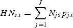 |
1 |
where Njs ∈ [0,1] represents compatibility of land cover j for nesting by species s. A Njs suitability value of 1 would indicate that land cover j provides habitat suitable for nesting (e.g. forest habitat in Table S2 in Supplementary Data, available online) while a score of 0·2 would indicate that effectively only 20 % of a parcel's area covered by land cover j provides suitable nesting habitat (e.g. coffee/pasture habitat).
Some land cover classes can provide habitat suitable for multiple nesting types. For example, in California, oak woodland habitat was scored as providing good habitat for wood-nesting, ground-nesting and cavity-nesting bees; in contrast, agricultural habitat was scored as providing lower quality habitat for ground-nesting bees, and no habitat for wood or cavity nesters.
For bee species or groups that span nesting types (e.g. a few groups such as Ashmiediella nest in the ground and in hollow stems) the nesting type was assigned to the habitat type that maximized its suitability for that bee species. In other words, if there are I nesting types, then Njs = max[NSsiNji, … , NSsINjI], where NSsi is the nesting suitability of nesting type i for species s and Nji is the suitability of land cover j for nesting type i. This analysis provides a map of nesting suitability (Fig. 2B). A nesting suitability score of 1 would indicate that the entire area of the parcel provides habitat suitable for nesting (e.g. forest habitat for a wood-nesting species) while a score of 0·2 would indicate 20 % of the parcel's area provides suitable nesting habitat (e.g. coffee/pasture habitat).
Floral resource
The proportion of suitable foraging habitat for pollinator species s nesting in parcel x given by HFsx ∈ [0,1] is calculated. It is assumed that foraging frequency in parcel x declines exponentially with distance (Cresswell et al., 2000), and that pollinators forage in all directions with equal probability. Therefore, parcels farther away from nest parcel x contribute less to total resource availability than parcels nearby. Floral resource production is also allowed to vary among K seasons. Data or expert opinion were used to assess the flight period and account for variation among pollinators in their K flight seasons, e.g. some are present in summer only, while others are present in multiple seasons. The overall floral resources available are calculated as a weighted sum across K seasons where the weight (wsk) ∈ [0,1] represents the relative importance of floral production in season k for species s (weights are in Table S4 for California and Table S6 for NJPA in Supplementary Data, available online). For the present analysis, the weights are based on expert opinion. Each wsk value is constrained such that
 |
1a |
This leads to the following prediction for the potential floral resources available to species s parcel x across K seasons, HF%:
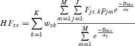 |
2 |
where pjm is the proportion of parcel m in land cover j, Dmx is the Euclidean distance between parcels m and x, αs is the typical foraging distance for species s (Greenleaf et al., 2007) and Fjs,k ∈ [0,1] represents suitability for foraging of land cover j for species s during season k (e.g Table S3 in Supplementary Data, available online). The use of Fjs,k permits attributing different resource levels to the same land-cover type for different bee species or guilds by season – for example, in California, riparian habitat produces important early-spring resources but many pollinator species are not yet flying at this time. By contrast, riparian habitat produces almost no summer resources. The numerator is the amount of distance-weighted resource summed across all M parcels. The denominator represents the maximum amount of forage in the landscape if all parcels had maximum available forage. This equation generates a distance weighted proportion of habitat providing floral resources within foraging range, normalized by the maximum total forage available within that range (Winfree et al., 2005). Using the normalized proportion controls for differences among pollinators that vary in their foraging radii, and allows total pollinator abundances to be estimated in subsequent model steps. This results in a pollinator floral resource map (Fig. 2C).
Pollinator source map
Since pollinator abundance is limited by both nesting and floral resources, the pollinator score on parcel x is simply the product of foraging and nesting such that Psx = HFsxHNsx.This score represents the location and relative abundance of pollinators available for crop pollination from parcel m and results in the source map.
Pollinator service map
Pollinators leave their nesting sites to forage in surrounding parcels, so farms surrounded by a higher abundance of nesting pollinators should experience higher abundances of pollinating visitors to their crops. The relative services provided to farms are calculated as the proportion of habitat from which pollinators arrive. To obtain the relative abundance of pollinators likely to travel from nest parcel m to forage on a crop in agricultural parcel o, we use the foraging framework described in eqn (2):
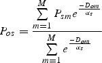 |
3 |
where Psm represents the relative abundance score of pollinator s on map unit m, Dom is distance between map unit m and farm o and αs is the average foraging distance of species s. Equation 3 is the distance-weighted proportion of M parcels that are occupied by foraging pollinators (Winfree et al., 2005). This score represents the relative abundance score of pollinators visiting each agricultural parcel and results in the pollinator services map (Fig. 2E).
To calculate the total pollinator score for farm o over all pollinators, Po, the normalized pollinator score is calculated for all pollinator guilds or species, such that:
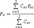 |
4a |
where Cos is 1 if the crop on farm o requires pollinator s, and 0 otherwise. This unweighted summation assumes that all pollinators are equally abundant. However, if some pollinators have higher background abundance than others, then a weighted average may be more appropriate such that:
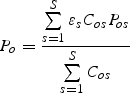 |
4b |
where εs represents the abundance of pollinator s in the landscape, relative to other pollinator species or guilds. The weights for each species can be determined by expert opinion or with empirical observations.
Model validation
To validate the model, its spatially explicit pollinator index is compared against total observed abundance, richness and estimates of pollen deposition in agricultural parcels of crops in three landscapes: coffee in Costa Rica, watermelon and sunflowers in California, USA and watermelon in NJPA, USA. In all cases, model parameters were derived independently of field validation data (e.g. estimates of typical foraging ranges, α), were derived from bee body size; floral availability by season and by bee species was estimated through expert assessment based on various studies other than those providing the validation data.
While it would be preferable to use quantitative, statistically derived estimates for all parameters, gathering these data is often difficult and expert opinion can be used to fill data gaps. Expert opinion has been applied and incorporated into predictive models in a number of fields such as nuclear engineering, aerospace, various types of forecasting (e.g. economic and meteorological, and snow avalanches, military intelligence, seismic risk and environmental risk from toxic chemicals; Clemen and Winkler, 1999). In a review of the use of expert opinion in lieu of statistical estimates, Keeney and von Winterfeldt (1989) stated that, ‘expert assessments are meant to be a complement to and motivation for [future] scientific studies and analysis, not as a substitute for either’. The authors have extensive experience in each of the three landscapes (Kremen, Greenleaf and Williams in California, Ricketts in Costa Rica and Kremen, Williams and Winfree in NJPA), so the estimates presented were derived through short discussions to reach consensus.
Costa Rica
The model was applied to an agricultural landscape in the Valle del General, Costa Rica, one of that country's major agriculture regions. The landscape is dominated by coffee farms, sugar cane, and cattle pasture, all of which surround hundreds of remnants of tropical/premontane moist forest (Janzen, 1983). Studies were conducted on 12 field sites on a large coffee farm (approx. 1100 ha) in the centre of this landscape.
High-resolution (1 m) aerial photographs, were classified into six major classes of land cover and resampled to 30-m spatial resolution, providing the proportion of each class within the 30-m parcel. These classes were then assigned values of nesting and floral resources (assuming a single flowering season) based on expert opinion (Table S1 in Supplementary Data, available online), informed by field work in the area (Ricketts, 2004; Brosi et al., 2008). Values were assigned on a relative scale, with 1 representing the maximum resources provided by any land-use type in the system, and 0·5 representing a land-use type that provides approximately half as many resources.
The most common visitors to coffee in this region are 11 species of native stingless bees (Meliponini) and the introduced, feral honey-bee, Apis mellifera. For the model, these 12 species were assigned to two nesting guilds based on expert opinion (Table S2 in Supplementary Data, available online). Lacking information on seasonality, a single flight season was assumed for all species. To estimate typical foraging ranges for each species (Table S2), inter-tegular spans were measured for ten museum specimens per species, and the statistical relationship presented by Greenleaf et al. (2007) was used.
During the flowering seasons of 2001 and 2002, Ricketts (2004) measured bee activity, pollen deposition and pollen limitation in 12 sites, varying from 10 m to 1600 m from the nearest major forest patch. These observations were compared against the model's predictions. The results were analysed with and without introduced honey-bees included because honey-bees interact with the landscape quite differently from native species; they are more generalized nesters, using a variety of substrates in agricultural areas, and have longer foraging ranges.
California
We applied the model to an agricultural landscape in the Central Valley of California, USA, where farms vary considerably in their distance to large tracts of natural habitat (oak woodland, chaparral scrub and riparian deciduous forest). Studies were conducted on watermelon (Kremen et al., 2002b, 2004) and sunflower (Greenleaf and Kremen, 2006) across this landscape.
The land-cover data were simplified from a 13-class supervised classification of Landsat TM data at 30 × 30 m resolution (described in detail in Kremen et al., 2004) into six classes. These classes were then assigned values of nesting and floral resources based on expert-opinion values (Table S3 in Supplementary Data, available online), informed by studies of bee–plant networks (Kremen et al., 2002a; Williams and Kremen, 2007) and bee-nesting densities (Kim et al., 2006) in the same landscape.
During the flowering season of 2001, bee visits were recorded at 12 watermelon sites and 11 sunflower sites. In 2002, bee visits were recorded at six additional sunflower sites (Greenleaf and Kremen, 2006). Total median pollen deposition was estimated for the watermelon data from separate work determining species-specific pollen deposition per visit (Kremen et al., 2002a). Each bee species in the study was characterized by its nesting habit based on expert opinion and the length of its flight period, based on over 12 000 bee specimens collected from 1999 to 2004 by pan-trapping and netting at flowers in this landscape (Table S4 in Supplementary Data; C. Kremen and R. W. Thorp, unpubl. res.; N. Williams, C. Kremen and R. W. Thorp, unpubl. res.). Typical foraging distances were calculated from measurements of inter-tegular span, using the regression in Greenleaf et al. (2007). For nearly all bee species, at least five individuals were measured but for a few species, only one measurement was used. Data on Apis mellifera, which are managed for pollination in this landscape, were removed prior to analysis for both sunflower and watermelon.
New Jersey and Pennsylvania
The model was applied to data collected at 23 farms within a 90 × 60 km area of central New Jersey and east-central Pennsylvania, USA. Land-cover data were based on 0·3-m-resolution aerial photographs taken in 2002 (New Jersey) and 2000 (Pennsylvania), and subsequently classified to six habitat classes (agriculture, suburban/urban development, woodland, open semi-natural grasslands, water, and other) at 30 × 30 m resolution. The New Jersey/Pennsylvania system spans a strong gradient in remaining native vegetation (deciduous woodland) cover at the landscape scale: the proportion of woodland at a 2 km radius around the study farm ranges from 8 % to 60 % (Winfree et al., 2008). However, in contrast to the Californian and Costa Rican systems, the remaining patches of forest are dispersed throughout the entire system, rather than forming a uni-directional gradient, such that no farm field in the study was >350 m from the nearest forest patch (Winfree et al., 2008).
Land-cover types were assigned nesting and floral resource availability values (Table S5 in Supplementary data available online) based on our previous studies of pollinator habitat use in this system (Winfree et al., 2007, 2008; Williams et al., unpubl. res.; Mandelik, Winfree and Kremen, unpubl. res.; Williams, Winfree and Kremen, unpubl. res.).Values were assigned on a relative scale, with 1 representing the maximum resources provided by any land-use type in the present system, and 0·5 representing a land-use type that provides half as many resources.
Aggregate native bee abundance on watermelon flowers was measured at 23 sites in 2005, using timed observation periods such that data were recorded in units of bee visits flower−1 time−1 (Winfree et al., 2007). Species richness was measured using the specimens collected from watermelon flowers at the end of the sampling period and subsequently identified to the species level. Information on nesting specialization and seasonality of the bees in the present system was compiled (Table S6 in Supplementary data available online) from the published literature (Hurd, 1979; Michener, 2000 ), from extensive personal observations (J. Ascher, American Museum of Natural History; T. Griswold, Utah State University), and for the seasonality data, from over 9000 museum specimens recorded by date and species. Wood-nesting bees were defined as those species obligatorily nesting in rotting wood, or in cavities in wood or twigs. Species nesting in soft-pithed stems were considered stem-nesting. Typical foraging distances were calculated from measurements of inter-tegular span (mean of five measurements per species, range 1–12), using the regression in Greenleaf et al. (2007).
Because data were collected on two separate days at each farm in NJPA, the data were analysed using ‘robust cluster’ regression (Stata version 7·0; Stata Corp., College Station, TX, USA). Robust clustering is a bootstrap procedure for sampling from data that are not independent within a cluster (sample dates within a farm) but that are independent across clusters (across farms).
Sensitivity analysis
Biological uncertainty exists, whether one derives parameter estimates from expert opinion or through formal study, so it is important to incorporate sensitivity analyses into model analyses to determine how uncertainty might influence interpretation of model results. It is particularly useful when models are used to guide the choice of a conservation management action. In this context, sometimes the magnitude of uncertainty may not influence the choice action and it is important to determine whether uncertainty inhibits confident decision making, thereby requiring additional study, or whether decisions are robust to uncertainty.
A sensitivity analysis is illustrated with the Costa Rican data to determine the extent to which the results depend on the precision and accuracy of the parameter estimates. In the present case, of interest is how uncertainty regarding expert estimates of nesting suitability, floral resource availability and statistically derived bee-dispersal distance influence the predicted pollinator abundance scores. If predicted values are found to be most sensitive at specific values, then further research is required to reduce this uncertainty before the model can be used by land managers with confidence.
The model predicts a parcel's pollinator abundance relative to other parcels on a landscape, so the sensitivity analysis focuses on these relative scores. Let  represent the normalized pollinator score on agricultural parcel o (from eqn 3 or 4) based on the original parameter estimates such that:
| 5 |
where Pmin and Pmax are the minimum and maximum pollinator service scores for all farms on the landscape. Let  represent the analogous normalized score on agricultural parcel o resulting from modified parameter combination c, and let
  be the average change in normalized scores from combination c such that:
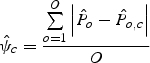 |
6 |
where O is the number of farms in the analysis. Because the model predicts relative rather than absolute pollinator abundance, the utility of the sensitivity analysis is currently limited to management of a single landscape, i.e. within Costa Rica.
Regression analysis is used to determine sensitivity, similar to the logistic regression approach used by McCarthy et al. (1995) in population viability analyses. The goal is to calculate how variation in each parameter affects estimates of a parcels' pollinator abundance, independent of all other parameters in the model. Given the number of parameters, exploring every combination of them is impractical. Instead, a sample of parameter combinations is created by selecting parameter values randomly from a uniform distribution, each within its range of uncertainty and then generating an estimated pollinator score  for each parcel.
To generate parameter combinations, a minimum and maximum were set for the range of parameter values and a random number drawn from a uniform distribution with this range (Table 2). For nesting suitability in Costa Rica the range was set based on the nesting suitability by land-cover scores ±0·1. For floral resources by land cover, the range was set based on the estimate ±0·1, with a maximum of 1 and minimum of 0. The bee dispersal estimates were based on the average from at least ten estimates so we drew a random number from a uniform distribution bounded by the minimum and maximum of those ten plus estimates to generate dispersal distances.
Table 2.
Results of sensitivity analysis for Costa Rican study
| Parameter | Estimate | Max | Min | δ (slope) | s.e.δ | Standardized regression coefficient (t-value) |
|---|---|---|---|---|---|---|
| Forage resource availability (Fj) | ||||||
| Forest | 1 | 1 | 0·9 | 4·550 | 1·303 | 3·493* |
| Coffee | 0·5 | 0·6 | 0·4 | 7·758 | 0·666 | 11·643* |
| Cane | 0 | 0·1 | 0 | 0·027 | 1·356 | 0·020 |
| Pasture/grass | 0·2 | 0·3 | 0·1 | 0·144 | 0·652 | 0·221 |
| Scrub | 0·3 | 0·4 | 0·2 | 0·553 | 0·657 | 0·842 |
| Bare | 0·1 | 0·2 | 0 | 0·300 | 0·663 | 0·453 |
| Built | 0·3 | 0·4 | 0·2 | 0·450 | 0·676 | 0·666 |
| Apis nesting suitability (Nj) | ||||||
| Forest | 1 | 1 | 0·9 | 0·046 | 1·300 | 0·035 |
| Coffee | 0·2 | 0·3 | 0·1 | 0·975 | 0·648 | 1·505 |
| Cane | 0 | 0·1 | 0 | 1·950 | 1·292 | 1·509 |
| Pasture/grass | 0·2 | 0·3 | 0·1 | 0·535 | 0·664 | 0·805 |
| Scrub | 0·3 | 0·4 | 0·2 | 0·784 | 0·674 | 1·162 |
| Bare | 0 | 0·1 | 0 | 2·896 | 1·302 | 2·224* |
| Built | 0·2 | 0·3 | 0·1 | 0·739 | 0·672 | 1·101 |
| Native nesting suitability (Nj) | ||||||
| Forest | 1 | 1 | 0·9 | 3·381 | 1·287 | 2·626* |
| Coffee | 0·1 | 0·2 | 0 | 0·067 | 0·650 | 0·102 |
| Cane | 0 | 0·1 | 0 | 0·382 | 1·318 | 0·290 |
| Pasture/grass | 0·1 | 0·2 | 0 | 0·259 | 0·683 | 0·379 |
| Scrub | 0·2 | 0·3 | 0·1 | 0·458 | 0·658 | 0·696 |
| Bare | 0·1 | 0·2 | 0 | 0·247 | 0·656 | 0·376 |
| Built | 0·1 | 0·2 | 0 | 0·640 | 0·659 | 0·972 |
| Foraging (metres) for each species (αs) | ||||||
| Apis mellifera | 663 | 776 | 562 | 0·001 | 0·001 | 1·467 |
| Huge Black 2002 | 214 | 239 | 191 | 0·007 | 0·003 | 2·376* |
| Melipona fasciata | 578 | 634 | 525 | 0·001 | 0·001 | 0·653 |
| Nannotrigona mellaria | 70 | 79 | 61 | 0·008 | 0·008 | 1·037 |
| Partamona cupira/Trigona fussipennis/Trigona corvina | 87 | 110 | 69 | 0·007 | 0·003 | 2·134* |
| Plebeia jatiformis | 28 | 30 | 25 | 0·027 | 0·024 | 1·131 |
| Plebia frontalis | 34 | 36 | 33 | 0·005 | 0·051 | 0·096 |
| Trigona (Tetragona) clavipes | 55 | 63 | 48 | 0·004 | 0·009 | 0·490 |
| Trigona (Tetragonisca) angustula | 22 | 24 | 20 | 0·013 | 0·029 | 0·453 |
| Trigona dorsalis | 60 | 66 | 54 | 0·006 | 0·011 | 0·544 |
| Trigona fulviventris | 77 | 82 | 73 | 0·046 | 0·015 | 3·158* |
| Trigonisca sp. | 21 | 23 | 20 | 0·043 | 0·051 | 0·829 |
The strength of the model's sensitivity is given by the standardized regression coefficients in the final column. These coefficients result from a multiple regression of the parameter value combinations on the average change in normalized pollination score,  .
.
* P < 0·05.
Table 1.
Descriptions of all parameters used in the model
| Parameter | Description |
|---|---|
| HN | Habitat suitability for nesting |
| HF | Habitat suitability for foraging |
| J | Number of land-cover types (each indexed by j) |
| Nj | Compatibility of habitat j for nesting |
| Fj | Compatibility of habitat j for foraging |
| M | Number of parcels in landscape (indexed by m) |
| D | Distance between parcels |
| α | Expected pollinator foraging distance |
| P | Pollinator abundance score |
| O | Number of farms (indexed by o) |
| x | Pollinator source parcel |
| S | Number of species (indexed by s) |
| I | Number of nesting types (indexed by i) |
| w | Weight describing importance of floral season for pollinator |
| K | Number of floral seasons (indexed by k) |
| C | Crops pollinator requirement |
| ε | Relative abundance of pollinator in landscape |
| ψ | Farms' average change in normalized scores (used for sensitivity analysis) |
By iterating this parameter draw process 1000 times, and then regressing the change in scores,  , against randomly varying parameters, sensitivity to each parameter was estimated while accounting for variation in the others. This linear regression method is an alternative to one in which there are a few discrete values for each parameter and a full-factorial experiment is run and analysed with an ANOVA. The drawback of this ANOVA approach is that there can be gaps in the parameter value combinations and not all parameter combinations can be assessed.
The sensitivity of each predictor variable is indicated by its standardized regression coefficient (t-value), calculated from the best fit of a multiple linear regression model: = δ0 + δ1x1 + … + δnxn, where xn are predictor variables (foraging distance, nesting suitability values, etc) and δn are the regression coefficients. The standardized regression coefficient is the t-value, the regression coefficient (slope of a line) divided by its standard error (δn/s.e.n; Cross and Beissinger, 2001). This is a unitless quantity that allows one to compare directly the sensitivity among parameters. Thus, parameters with the largest t-values indicate greatest sensitivity of the model to that parameter. Since the parameter combinations were created randomly, it also accounts for potential interactions among model parameters (Cross and Beissinger, 2001). The standard error for one model parameter is caused by the dependence of
  on other parameters and the significance of the slope is calculated using a two-tailed t-distribution (a t-value greater than 1·9 or less than –1·9 is significant at P < 0·05).
RESULTS
Model validation
In the California landscape, the model predicted at least 55 % of the variance among farms in observed aggregate bee abundance for watermelon and both years sunflowers were sampled (Fig. 3A). Similarly, the model predicted at least 63 % of the variance in richness of native bees on watermelon and sunflower (Fig. 3D). Model predictions were also strongly related to estimated pollen deposition on watermelon from native bees (Fig. 3G; R2 = 0·56), a more direct measure of pollination services (Kremen et al., 2002a, 2004; Ricketts, 2004; Winfree et al., 2007).
Fig. 3.

Comparison of predicted and observed pollination scores at three study sites. In each site the model's predicted abundance we compared with pollinator abundance (A, California; B, Costa Rica; C, NJPA), native bee species richness (D, California; E, Costa Rica; F, NJPA), and pollen deposition (G, watermelon only in California; H, Costa Rica; I, NJPA). Note that vertical scales vary between graphs.
For the Costa Rican landscape, the model predicted 80 % of the variance in observed aggregate bee abundance without honey-bees (Fig. 3B) and 62 % of native bee richness (Fig 3E). The model's predictions for landscape provision of pollinators were less strongly related to field measurements of pollen deposition on coffee stigmas (Fig. 3H; R2 = 0·20).
In New Jersey, the model did not provide a good a fit to observed data on either aggregate abundance (F = 0·98, R2 = 0·04, Fig. 3C), richness (F = 0·40, R2 = 0·01; Fig. 3F) or pollen deposition (F = 0·23, R2 = 0·01, Fig. 3I).
Sensitivity analysis
The sensitivity analysis was conducted solely on the Costa Rica data set (Table 2 because it has a simpler data structure (fewer nesting and floral resource parameters). The results indicate that a farm's normalized pollinator score,  , is most sensitive to foraging resources present in coffee habitat (t-value = 11·65; P < 0·05).
  is also sensitive to uncertainty in foraging distance for a few species with relatively moderate foraging ranges (e.g. 70–250 m), but not to species with smaller or greater estimated foraging ranges. Finally, uncertainty in estimates for nesting and floral resources in forest habitat also affected relative pollinator service (nesting: t-value = 2·626, P < 0·05; floral: t-value = 3·493, P < 0·05).
DISCUSSION
By formalizing the conceptual presentation of mobile agent-based ecosystem services (Kremen et al., 2007) and integrating the knowledge from a large body of work, the model provides an important step in evaluating the landscape contributions to pollinator populations and crop pollination. It represents the first spatially-explicit model of landscapes for their capacity to support bees and the match between empirical and modelling results strongly supports the modelling framework. The model accurately predicted the relative abundances and richness of native pollinators in two of three landscapes, capturing a minimum of 55 % of the observed variance among farms for pollinator abundance and richness on sunflowers and watermelon in California and on coffee in Costa Rica (Fig. 3). While the model did not predict pollinator abundance and richness in the NJPA data set, it may be due to low variance in this system, or to the resolution of land-cover data (relative to the scale of the ecological phenomenon in this landscape; see below) rather than faulty model assumptions. The model is relatively simple and designed to be used anywhere where sufficient land-cover data exist along with the ability to code them in terms of floral and nesting resource availability. While land-cover data for most places are widely available, the knowledge necessary to code land-use types and estimate pollinator foraging ranges and seasonality may vary; therefore we have designed a model that is flexible. For example, the model of pollinator communities in California accounted for four nesting types and three seasons of floral resources, while the model of Costa Rica used only two nesting types and only one season, because the knowledge base to resolve nesting and seasonal guilds more finely was not available.
In future work, it is planned to develop further the model as a guide to landscape-level management for pollinators. First, this model will be applied to a much larger set of crop studies conducted at the landscape scale (viz. studies in Ricketts et al., 2008). Secondly, a landscape metric has been used as a proxy for abundance, so the larger set of studies can be used to derive and parameterize a more explicit functional relationship between this landscape metric (floral and nesting resources) and abundance are warranted. If one assumes a liner relationship (Type I) between the metric and abundance, the model may underestimate abundance at the edges, while a saturating relationship (Type II or III) between the metric and abundance may be more appropriate. Thirdly, using statistical techniques, the landscape-level outputs of the model (pollinator relative abundance) will be related to the observed measure of pollination services in each study (e.g. pollen deposition, pollen limitation) to attempt to develop a direct relationship between landscape and yield effects via pollinator abundances. Finally, by manipulating modelled landscapes (e.g. by increasing floral or nesting resources in different spatial configurations), the effects on pollinator abundance, richness and service delivery can be estimated across a range of changes in resources, and generalities looked for across landscapes in the density and arrangement of resources needed to protect pollinators and/or provide adequate pollination services. This modelling exercise would inform efforts to preserve existing habitats within degraded landscapes and also guide spatial planning of priorities for habitat restoration. Similar to the sensitivity analysis of model parameters, analyses exploring the sensitivity of modelled pollination services to resource patchiness at different grain sizes or to different landscape configurations are also envisioned.
The model was unable to predict pollinator abundances in the New Jersey landscape. It is hypothesized that this may be due to the availability of fine-scale floral and nesting resources on and surrounding the farms, which was not captured in the land-cover data. In order to standardize the methods across the data sets included in this study, the same 30-m resolution for the land cover input data was used for all three study systems. In deriving 30-m resolution for Costa Rica and California, it was possible to account for proportions of habitat within each parcel, e.g. for Costa Rica the proportion of each land-cover class within the 30-m parcel was included. But finer-scale data were not available at the time of the analysis so the NJPA parcel had only one land-cover class per 30-m parcel. Furthermore, the NJPA landscapes had greater habitat heterogeneity to begin with, so the simplification to 30-m pixels probably entailed a greater loss of detail in this system than in others. The CA and Costa Rican landscapes have larger grain sizes and are characterized by large expanses of agriculture contrasted with continuous blocks of natural habitat. In contrast, in NJPA, grain sizes are smaller with the agricultural, natural and other habitat types being inter-digitated at a small spatial scale. Furthermore, habitat heterogeneity is high even within a habitat type; for example, many agricultural fields contain weedy fallow areas that would not be separately identified in the land-cover data. In sum, although bees are known to respond to resource availability at scales smaller than the 30-m parcel size (Morandin and Winston, 2006; Albrecht et al., 2007; Kohler et al., 2007), the simplification to a 30-m resolution may not matter for landscapes where there is little heterogeneity at this scale, whereas the same resolution may result in inaccuracies in landscapes with greater heterogeneity at relatively smaller scales.
Two other results support this hypothesis for the model's poor fit in the NJPA landscape. First, the sensitivity analysis of the Costa Rica landscape indicates model predictions are sensitive to floral resources provided within coffee or crop habitat (Table 2), i.e. to resources distributed at a small scale. Secondly, in the NJPA system and using the same land-cover data, it has not been possible to detect any relationship between land cover variables and pollinator abundance, richness or services (Winfree et al., 2007, 2008). These results contrast with the majority of other study systems (Ricketts et al., 2008), and again suggests that the land-cover data in this system does not capture the relevant variables at the appropriate scale.
An alternative explanation for the poor fit is that among NJPA farms there simply may not be enough variation to explain in their pollinator communities, in their surrounding landscapes or both. If this were the case, comparisons of among-farm variation in the model prediction and observed data would reveal higher variation in Costa Rica and California compared with NJPA. A post hoc comparison of the abundance, richness and pollen deposition, as well as the landscape model's prediction, was performed using the variation in these observed variables divided by the mean squared. This is a unitless quantity, often called the opportunity for selection (Arnold and Wade, 1984), and removes the expected scaling that occurs between the mean and variance of a distribution, thus allowing comparisons among quantities that may differ in their units or mean values.
The post hoc comparison reveals that indeed Costa Rica and California have much higher standardized variances in both the observed and predicted values and that limited variation in the landscape surrounding NJPA farms may explain the model's poor fit (Fig. 4). The NJPA farms show much lower variation for all three observed pollination measures and the pollinator service scores provided by the landscape analysis is consistent with the observation of little variation (Fig. 4A). Furthermore, the variance in the observed variables explained by the model tends to increase with increasing variability in the landscape (Fig. 4B) lending support to the idea there is too little variation in the NJPA landscape to pick a strong effect of the landscape. We suggest using the variance-to-mean2 ratio in other studies for future comparisons.
Fig. 4.

A post hoc cross-site comparison of variation in model prediction and observed pollinator abundance, richness and pollen deposition. There is much greater variation across farms with the studies in California and Costa Rica compared with NJPA (A). This may explain why the model does a better job explaining pollinator communities and pollination in California and Costa Rica when compared with NJPA (B).
Despite the promising results in matching data to predictions in two of three landscapes, there are structural limitations of the model. First, it is limited to predicting relative pollinator abundance as a function of resources related to land cover, which is only one of many potential contributors to pollinator population and pollination services, e.g. pesticides. Also, while quantitative, it cannot project pollinator abundance over time, but rather assumes population stasis given a particular landscape configuration. In other words, the model does not provide an estimate of pollinator population viability or predict pollinator temporal dynamics or interaction of time and space through metapopulation dynamics. As such, it does not incorporate stochastic events, which may influence both long-term pollinator population dynamics and, ultimately, crop yield. With more information, one could expand the model to include these factors, in which case, the model presented here would simply be one input to account for resource availability while other inputs would account for other factors, e.g. weather, pesticides, etc.
Predicting crop yield from the landscape pattern is a final goal, and more research is clearly needed in this area (Kremen, 2005; Morandin and Winston, 2006; Kremen et al., 2007). Translating from pollinator abundance to pollinator influence on crop yield will be limited in many cases by four major gaps in our understanding of pollinator-yield effects. The first three of these are related to the plant breeding system and only the last relates to the plant–pollinator interaction. First, the functional form of the relationship between increased number or quality of pollen grains deposited and yield is often not known. Secondly, this functional form is likely to vary significantly among crop varieties and species as some species may rely more or less on outcross pollen. Thirdly, this functional form may vary under different conditions of resource limitation (e.g. water, nutrients). Finally, the relationship between pollinator abundance and the amount and quality of pollen delivered is influenced by pollinator foraging behaviour, across scales from within the flower, to across flower patches and to foraging decisions over the entire landscape (Klein et al., 2007; Kremen et al., 2007; Ricketts et al., 2008).
Once the relationship between pollinator abundance and crop yield is parameterized (i.e. the input–output relationships are understood), it can be used to predict the economic value of pollination or any other input, based on their relative contributions to crop yield. Using production functions in this way will result in an estimate of the economic value of pollinators at each farm. It is most likely of interest, however, to estimate the value of the habitats in the landscape that support these pollinators. For this, the ecological models described here can be used to attribute economic value realized on farms back to the pollinator-supporting habitats. Once this is done, spatially-explicit, optimization techniques and heuristics already exist (Polasky et al., 2005, 2008) and provide a decision structure with which to evaluate land-use plans. When combined with decision analysis, the model can be used to evaluate alternate land-use plans designed to promote pollinator services and maximize economic return from the crop.
While the economic value of pollinators for agricultural production is important to determine, we recognize that the motivation to estimate each bee species' monetary value is simply a strategy to ensure their conservation. The quantitative model presented here fills an important gap in conservation planning. Incorporating landscape models into land-use planning for multi-species conservation is an ongoing area of research but most of these models exclude pollinators focus solely on vertebrates (birds, mammals and herps) and those that have included pollinators do not incorporate much biological detail (Chan et al., 2006). Estimating the social value of pollinators (financial or otherwise) is not a scientific exercise (Gregory et al., 2006), but the scientific modelling framework developed here can be applied to inform management of landscapes where pollinator conservation is a fundamental objective, rather than the means to an economic end.
SUPPLEMENTARY DATA
Supplementary data is available online at www.aob.oxfordjournals.org/ and consists of the following tables. Table S1: Floral resource and nesting suitability values for land-use land cover in Costa Rica. Table S2: Species foraging distances and nesting suitability values for Costa Rica. Table S3: Nesting suitability and floral resource values for land cover in California. Table S4: Species and guilds' expected foraging distance, nesting suitability estimates for species visiting watermelon and/or sunflower in California. Table S5: Nesting suitability and floral resource values for land cover in New Jersey and Pennsylvania. Table S6: Species and guilds' expected foraging distance, nesting suitability estimates for species visiting watermelon in New Jersey and Pennsylvania.
ACKNOWLEDGEMENTS
This work was facilitated by McDonnell Foundation 21st Century and University of California Chancellor's Partnership awards to C.K., and by two National Center for Ecological Analysis and Synthesis working groups (Restoring an ecosystem service to degraded landscapes: native bees and crop pollination; PI's C.K. and N.M.W. Natural Capital Project) supported by NSF (grant no. DEB-00-72909), the University of California at Santa Barbara, and the State of California. Kirsten Almberg helped with figures and Jaime Florez provided measurements of inter-tegular spans for Costa Rican bees. Peter Kareiva, Erik Nelson, Berry Brosi and Kai Chan all provided input in early development of the model.
LITERATURE CITED
- Albrecht M, Duelli P, Müller C, Kleijn D, Schmid B. The Swiss agri-environment scheme enhances pollinator diversity and plant reproductive success in nearby intensively managed farmland. Journal of Applied Ecology. 2007;44:813–822. [Google Scholar]
- Arnold SJ, Wade MJ. On the measurement of sexual and natural selection: theory. Evolution. 1984;38:709–719. doi: 10.1111/j.1558-5646.1984.tb00344.x. [DOI] [PubMed] [Google Scholar]
- Brosi BJ, Daily GC, Shih TM, Oviedo F, Duràn G. The effects of forest fragmentation on bee communities in tropical countryside. Journal of Applied Ecology. 2008;45:773–783. [Google Scholar]
- Chan KMA, Shaw MR, Cameron DR, Underwood EC, Daily GC. Conservation planning for ecosystem services. PLoS Biology. 2006;4:e379. doi: 10.1371/journal.pbio.0040379. [DOI] [PMC free article] [PubMed] [Google Scholar]
- Clemen RT, Winkler RL. Combining probability distributions from experts in risk analysis. Risk Analysis. 1999;19:187–203. doi: 10.1111/0272-4332.202015. [DOI] [PubMed] [Google Scholar]
- Cresswell JE, Osborne JL, Goulson D. An economic model of the limits to foraging range in central place foragers with numerical solutions for bumblebees. Ecological Entomology. 2000;25:249–255. [Google Scholar]
- Cross PC, Beissinger SR. Using logistic regression to analyze the sensitivity of PVA models: a comparison of methods based on African wild dog models. Conservation Biology. 2001;15:1335–1346. [Google Scholar]
- Gallai N, Vaissière BE, Potts SG, Salles J. Assessing the monetary value of global crop pollination services. In: Kareiva P, Daily G, Ricketts T, Tallis H, Polasky S, editors. The theory and practice of ecosystem service valuation in conservation. Oxford: Oxford University Press (in press); 2009. [Google Scholar]
- Gathmann A, Tscharntke T. Foraging ranges of solitary bees. Journal of Animal Ecology. 2002;71:757–764. [Google Scholar]
- Greenleaf SS, Kremen C. Wild bee species increase tomato production and respond differently to surrounding land use in Northern California. Biological Conservation. 2006;133:81–87. [Google Scholar]
- Greenleaf S, Williams N, Winfree R, Kremen C. Bee foraging ranges and their relationship to body size. Oecologia. 2007;153:589–596. doi: 10.1007/s00442-007-0752-9. [DOI] [PubMed] [Google Scholar]
- Gregory R, Failing L, Ohlson D, McDaniels TL. Some pitfalls of an overemphasis on science in environmental risk management decisions. Journal of Risk Research. 2006;9:717–735. [Google Scholar]
- Hines HM, Hendrix SD. Bumble bee (Hymenoptera: Apidae) diversity and abundance in tallgrass prairie patches: effects of local and landscape floral resources. Environmental Entomology. 2005;34:1477–1484. [Google Scholar]
- Hoehn P, Tscharntke T, Tylianakis JM, Steffan-Dewenter I. Functional group diversity of bee pollinators increases crop yield. Proceedings of the Royal Society B: Biological Sciences. 2008;275:2283–2291. doi: 10.1098/rspb.2008.0405. [DOI] [PMC free article] [PubMed] [Google Scholar]
- Hurd PDJ. Superfamily Apoidea. In: Krombein KV, Hurd PDJ, Smith DR, Burks BD, editors. Catalog of Hymenoptera in America North of Mexico. Washington, DC: Smithsonian Institution Press; 1979. [Google Scholar]
- Janzen D. Costa Rican natural history. Chicago, IL: University of Chicago Press; 1983. [Google Scholar]
- Keeney RL, von Winterfeldt D. On the uses of expert judgment on complex technical problems. IEEE Transactions on Engineering Management. 1989;36:83–86. [Google Scholar]
- Kevan PG, Clark EA, Thomas VG. Insect pollinators and sustainable agriculture. American Journal of Alternative Agriculture. 1990;5:12–22. [Google Scholar]
- Kim J, Williams N, Kremen C. Effects of cultivation and proximity to natural habitat on ground-nesting native bees in California sunflower fields. Journal of the Kansas Entomological Society. 2006;79:309–320. [Google Scholar]
- Klein AM, Steffan-Dewenter I, Tscharntke T. Fruit set of highland coffee increases with the diversity of pollinating bees. Proceedings of the Royal Society of London Series B: Biological Sciences. 2003;270:955–961. doi: 10.1098/rspb.2002.2306. [DOI] [PMC free article] [PubMed] [Google Scholar]
- Klein A-M, Vaissiére BE, Cane JH, et al. Importance of pollinators in changing landscapes for world crops. Proceedings of the Royal Society of London Series B: Biological Sciences. 2007;274:303–313. doi: 10.1098/rspb.2006.3721. [DOI] [PMC free article] [PubMed] [Google Scholar]
- Knight ME, Martin AP, Bishop S, et al. An interspecific comparison of foraging range and nest density of four bumblebee (Bombus) species. Molecular Ecology. 2005;14:1811–1820. doi: 10.1111/j.1365-294X.2005.02540.x. [DOI] [PubMed] [Google Scholar]
- Kohler F, Verhulst J, Knop E, Herzog F, Kleijn D. Indirect effects of grassland extensification schemes on pollinators in two contrasting European countries. Biological Conservation. 2007;135:302–307. [Google Scholar]
- Kremen C. Managing ecosystem services: what do we need to know about their ecology? Ecology Letters. 2005;8:468–479. doi: 10.1111/j.1461-0248.2005.00751.x. [DOI] [PubMed] [Google Scholar]
- Kremen C, Chaplin-Kramer R. Insects as providers of ecosystem services: crop pollination and pest control. In: Stewart AJA, New TR, Lewis OT, editors. Insect conservation biology: Proceedings of the Royal Entomological Society's 23rd Symposium. Wallingford: CABI Publishing; 2007. [Google Scholar]
- Kremen C, Bugg RL, Nicola N, Smith SA, Thorp RW, Williams NM. Native bees, native plants and crop pollination in California. Fremontia. 2002a;30:41–49. [Google Scholar]
- Kremen C, Williams NM, Thorp R. W. Crop pollination from native bees at risk from agricultural intensification. Proceedings of the National Academy of Sciences of the USA. 2002b;99:16812–16816. doi: 10.1073/pnas.262413599. [DOI] [PMC free article] [PubMed] [Google Scholar]
- Kremen C, Williams NM, Bugg RL, Fay JP, Thorp RW. The area requirements of an ecosystem service: crop pollination by native bee communities in California. Ecology Letters. 2004;7:1109–1119. [Google Scholar]
- Kremen C, Williams NM, Aizen MA, et al. Pollination and other ecosystem services produced by mobile organisms: a conceptual framework for the effects of land-use change. Ecology Letters. 2007;10:299–314. doi: 10.1111/j.1461-0248.2007.01018.x. [DOI] [PubMed] [Google Scholar]
- McCarthy MA, Burgman MA, Ferson S. Sensitivity analysis for models of population viability. Biological Conservation. 1995;73:93–100. [Google Scholar]
- Michener C. The bees of the world. Baltimore, MD: Johns Hopkins University Press; 2000. [Google Scholar]
- Morandin LA, Winston M. L. Pollinators provide economic incentive to preserve natural land in agroecosystems. Agriculture, Ecosystems & Environment. 2006;116:289–292. [Google Scholar]
- National Research Council of the National Academies. Status of pollinators in North America. Washington, DC: National Academy Press; 2006. [Google Scholar]
- Polasky S, Nelson E, Lonsdorf EV, Fackler P, Starfield T. Conserving species in a working landscape: efficient land use with biological and economic objectives. Ecological Applications. 2005;15:1387–1401. [Google Scholar]
- Polasky S, Nelson E, Camm J, et al. Where to put things? Spatial land management to sustain biodiversity and economic returns. Biological Conservation. 2008;141:1505–1524. [Google Scholar]
- Potts SG, Vulliamy B, Dafni A, Ne'eman G, Willmer PG. Linking bees and flowers: how do floral communities structure pollinator communities? Ecology. 2003;84:2628–2642. [Google Scholar]
- Potts SG, Vulliamy B, Roberts S, et al. Role of nesting resources in organising diverse bee communities in a Mediterranean landscape. Ecological Entomology. 2005;30:78–85. [Google Scholar]
- Ricketts TH. Tropical forest fragments enhance pollinator activity in nearby coffee crops. Conservation Biology. 2004;18:1262–1271. [Google Scholar]
- Ricketts TH, Regetz J, Steffan-Dewenter I, et al. Landscape effects on crop pollination services: are there general patterns? Ecology Letters. 2008;11:499–515. doi: 10.1111/j.1461-0248.2008.01157.x. [DOI] [PubMed] [Google Scholar]
- Stokstad E. The case of the empty hives. Science. 2007;316:970–972. doi: 10.1126/science.316.5827.970. [DOI] [PubMed] [Google Scholar]
- Tepedino VJ, Stanton NL. Diversity and competition in bee-plant communities on short-grass prairie. Oikos. 1981;36:35–44. [Google Scholar]
- Westrich P. Habitat requirements of central European bees and the problems of partial habitats. In: Matheson A, Buchmann SL, O'Toole C, Westrich P, Williams IH, editors. The conservation of bees. London: Academic Press; 1996. pp. 1–16. [Google Scholar]
- Williams N, Kremen C. Floral resource distribution among habitats determines productivity of a solitary bee, Osmia lignaria, in a mosaic agricultural landscape. Ecological Applications. 2007;17:910–921. doi: 10.1890/06-0269. [DOI] [PubMed] [Google Scholar]
- Winfree R, Kremen C. Are ecosystem services stabilized by differences among species? A test using crop pollination. Proceedings of the Royal Society of London. 2009;276:229–237. doi: 10.1098/rspb.2008.0709. [DOI] [PMC free article] [PubMed] [Google Scholar]
- Winfree R, Dushoff J, Crone E, et al. Testing simple indices of habitat proximity. American Naturalist. 2005;165:707–717. doi: 10.1086/430009. [DOI] [PubMed] [Google Scholar]
- Winfree R, Williams NM, Dushoff J, Kremen C. Native bees provide insurance against ongoing honey bee losses. Ecology Letters. 2007;10:1105–1113. doi: 10.1111/j.1461-0248.2007.01110.x. [DOI] [PubMed] [Google Scholar]
- Winfree R, Williams NM, Gaines H, Ascher JS, Kremen C. Wild bee pollinators provide the majority of crop visitation across land-use gradients in New Jersey and Pennsylvania, USA. Journal of Applied Ecology. 2008;45:793–802. [Google Scholar]