A New Approach to the Quantification of Degree of Reciprocity in Distylous (sensu lato) Plant Populations

Abstract

Background and Aims

Although evolution of sexual polymorphism has been traditionally analysed using discrete characters, most of these polymorphisms are continuous. This is the case of heterostyly. Heterostyly is a floral polymorphism successfully used as a model to study the evolution of the sexual systems in plants. It involves the reciprocal positioning of anthers and stigmas in flowers of different plants within the same population. Studies of the functioning of heterostyly require the quantification of the degree of reciprocity between morphs of heterostylous species. Some reciprocity indices have been proposed previously, but they show significant limitations that need to be dealt with. This paper analyses these existing indices, and proposes a new index that aims to avoid their main problems (e.g. takes into account population variability and offers a single value per population).

Methods

The new index is based on the comparison of the position of every single sexual organ in the population with each and every organ of the opposite sex. To carry out all the calculations, a macro was programmed with MS^®Visual Basic in MS^® Excel. The behaviour of the index is tested using hypothetical data to simulate different situations of dimorphic populations; the index is also tested with some actual populations of different species of the genus Lithodora.

Results and Conclusions

The index of reciprocity proposed here is a sound alternative to previous indices: it compares stigma–stamen height gaps for all potential crosses in the population, it comprises stigma–stamen distance as well as dispersion, it is not skewed by the more frequent sex, and it can be meaningfully compared between populations and species. It has produced solid results for both hypothetical and natural populations.

INTRODUCTION

The study of flower polymorphisms has attracted biologists for years because they are model systems to investigate general questions concerning the evolutionary biology of sex. Among these polymorphisms, heterostyly has been proved to be one of the most explanatory (e.g. see Barrett, 1992; Lloyd and Webb, 1992a; Barrett and Hodgins, 2006). Heterostyly is a genetic polymorphism such that plant populations are composed of two (distyly) or three (tristyly) morphs that differ reciprocally in the heights of stigmas and anthers (Barrett, 1992). Traditionally, reciprocal herkogamy between morphs has been considered as the necessary and sufficient condition to characterize a plant as heterostylous (Ganders, 1979; Lloyd and Webb, 1992a; Barrett, 2002). However, further differences between the various morphs may include incompatibility reactions and ancillary characters (for a review, see Dulberger, 1992). Perfect reciprocal herkogamy in a population is achieved when the anthers of one morph are positioned at the same level as the stigmas of the other. Ideally, this should be true for each anther and stigma of all flowers in the population, but actually different degrees of reciprocal herkogamy between morphs can be found in natural populations of heterostylous species.

Since Darwin (1877) and Hildebrand (1864) started to study the evolutionary pathways of this polymorphism, some hypotheses have been proposed to explain the evolution of heterostyly (Baker, 1966; Charlesworth and Charlesworth, 1979; Ganders, 1979; Lloyd and Webb, 1992a, b; Richards, 1998). In all these models, transitions among different degrees of reciprocity along the evolutionary pathway leading to heterostyly are present; for example, starting either from a situation of herkogamy (Lloyd and Webb, 1992a, b) or homostyly (Charlesworth and Charlesworth, 1979), reciprocal herkogamy increases at any step of a given evolutionary sequence leading to heterostyly. Avoidance of self-pollination and promotion of intermorph pollination are the major selective forces responsible for the reciprocity of position of the sexual organs (Darwin, 1877; Lloyd and Webb, 1992b). Thus morphological adjustment of reciprocity of sexual traits among floral morphs has an enormous relevance in the stability of heterostyly since the proportion of legitimate pollen deposited by pollinators on appropriate stigmas of herkogamous flowers should be greater as they become more reciprocal (see Lau and Bosque, 2003). In this sense, shifts from tristyly to distyly in Oxalis alpina come along with differences in reciprocal herkogamy due to the relocation of mid-level anthers to maximize legitimate crosses after the loss of mid-stigmas (Weller, 1992). The same happens in Pemphis acidula (Lewis and Rao, 1971) (for Decodon verticillatus, see also Eckert and Mavraganis, 1996).

Most works on evolution of heterostyly have considered this character as discrete, but some others acknowledge reciprocal herkogamy as a quantitative character (e.g. Lloyd et al., 1990; Richards and Koptur, 1993; Eckert and Barrett, 1994) proposing indices to get a quantification of reciprocal herkogamy (i.e. reciprocity sensu Richards and Koptur, 1993). Some of those indices also take into account precision in the organ levels (Eckert and Barrett, 1994) since accuracy in pollination, and more concretely in disassortative crosses, would decrease if the organ height of one morph is out of line with the other. Up to the present, the indices have been used to confirm the heterostylous status of certain species or populations by comparing them with other reference species (Thompson et al., 1996; Massinga et al., 2005). From our point of view, a reciprocity index is also useful to trace the evolutionary steps leading to heterostyly along known phylogenetical reconstructions; to be correlated with population fitness measures in order to test if the most reciprocal populations are more successful than the less reciprocal, or just to decide if a given population is heterostylous or style dimorphic and to what extent. As an example of its importance, several studies have established that high rate of disassortative (between morphs) crosses are needed to maintain the proportion of morphs in the population (Barrett, 1990; Baker et al., 2000; Arroyo et al., 2002; Thompson et al., 2003). Although it also depends on the behaviour of pollinators (Pérez et al., 2007), such disassortative crosses are more likely to occur in highly reciprocal populations (Lau and Bosque, 2003).

Analysing previous indices

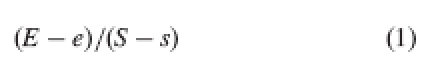
Eckert and Barrett (1994) proposed a simple index to quantify overall population reciprocity, but, as they themselves state, this index shows some limitations. The main limitation derives from the fact that the index is based on the comparison of the distances between organs of the same sex in the different morphs; therefore, as they state, the index measures ‘equality of inter-organ distances rather than true reciprocity’. In other words, a population in which the distance between morph-L and morph-S anthers is the same as the distance between morph-L and morph-S stigmas will be classed as perfectly reciprocal, even if no pair of flowers has any matching stigma or anther heights. Another drawback is that the index is calculated from a single height value (a mean or a single datum) for each organ level and sex:

1

where E is stamen height at level L (long), i.e. in flowers of morph-A plants; S is stigma height at level L, i.e. in flowers of morph-B plants; e is stamen height at level S (short), i.e. in flowers of morph-A plants; and s is stigma height at level S, i.e. in flowers of morph-B plants.

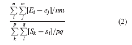
Perfect reciprocity as measured by this index has a value of one. As noted, though, the index is calculated from single height values (not specified by the authors), and thus takes no account of within-population variability. A more accurate approach would be to consider each single comparison between each stamen and all stamens of the other morph, and the same for stigmas. The average of the absolute values of all of these one-to-one comparisons would be a more accurate indicator of reciprocity in the population:

2

where n is the number of stamens at level L; p is the number of stigmas at level L; m is the number of stamens at level S; and q, the number of stigmas at level S (see Table 1 for list of abbreviations).

Table 1.

Abbreviations used in equations

E	Stamen height at level L (long), i.e. in flowers of morph-A plants
S	Stigma height at level L, i.e. in flowers of morph-B plants
e	Stamen height at level S (short), i.e. in flowers of morph-A plants
s	Stigma height at level S, i.e. in flowers of morph-B plants
n	Total number of all single stamens (i) at level L
p	Total number of all single stigmas (k) at level L
m	Total number of all single stamens (j) at level S
q	Total number of all single stigmas (l) at level S
P	Precision
CVL	Coefficient of variation at level L
CVS	Coefficient of variation at level S
R	Relative reciprocity at a given level (Richards and Koptur, 1993)
R	Mean relative reciprocity at a given level (modified from Richards and Koptur, 1993)
ra	Mean relative reciprocity at level a (as proposed here)
X	Average of heights of all organs (stigmas and stamens) in the population
r	Overall reciprocity of the population
rL	Relative reciprocity at level L
rS	Relative reciprocity at level S
sdra	Standard deviation of the height gaps at level a
sdrL	Standard deviation of height gaps at level L
sdrS	Standard deviation of height gaps at level S

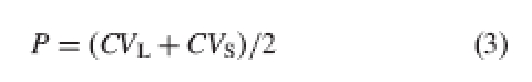
In fact, Eckert and Barrett (1994) themselves acknowledged the need to take into account the dispersion of height values around the mean. To this end, they propose a measure of precision obtained as the average of the coefficients of variation in the heights of both organs (stamens and styles) at the different levels, as follows (adapted for a distylous population):

3

where P is precision, CV_L is the coefficient of variation at level L, and CV_S is the coefficient of variation at level S.

This is a clear advance, but still has a major drawback: the CV value at each level will be skewed towards the most numerous of the sexes (stamens), i.e. it will not be a measure of the dispersion of ‘possible crosses’, but mainly of the dispersion of the stamens. Furthermore, we consider that it would be useful to have a single index that integrates both components (quantification of reciprocal herkogamy and precision, see below).

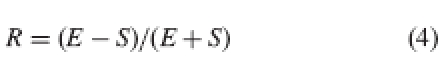
Another approach is that proposed by Richards and Koptur (1993), who define relative reciprocity (at a given level) as the distance between stigmas and stamens at that level relative to the total height of stigmas plus stamens at that level:

4

where R is relative reciprocity at a given level, E is stamen height at that level and S is stigma height at that level.

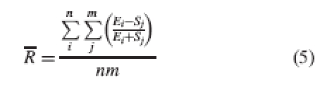
Values vary between 1 and –1, with zero indicating perfect reciprocity. In the case of distylous species, the results for each level can be plotted on an x–y graph, allowing visual comparison between populations and species. Another advantage of this index is that it measures true reciprocity: R will be zero only when (E – S) is zero, that is to say, when anther height equals stigma height at that level. This is not the case with the index of Eckert and Barrett (1994). The possibility of visual comparison offered by this index is especially useful for comparing populations, but also has some drawbacks. First, like Eckert and Barrett's, this index uses a single representative value for each sex and level. It would be more accurate to compare each organ in the population with all possible crosses in order to avoid inaccuracy when means or representative single values are used to represent populations with skewed distributions and/or outliers; then average all those comparisons to obtain a relative reciprocity index as follows:

5

where R is the mean relative reciprocity at a given level, E is stamen height at that level; n is number of stamens at that level, S is stigma height at that level and m is number of stigmas at that level.

Secondly, although this index is visually informative, since the denominator of reference for each level is different (E + S for that level), the relative reciprocity indices obtained are not comparable between levels within the same population: even if the distance between stigma and stamen heights is the same at both levels, relative reciprocity for the long level will always be lower simply because E + S is higher at that level.

Thirdly, as with Eckert and Barrett's, this index fails to address the problem of data dispersion (precision) and does not provide a single integrated measure of reciprocity.

A reliable index of reciprocity is therefore needed in the studies of the evolution of heterostyly. The aim in this paper is to propose an alternative index that (a) offers a single quantitative value that can be used to compare species and populations, and (b) that takes into account both reciprocity (difference between mean stigma and stamen heights) and precision (dispersion of the single value around those means). In a system with differences in only one dimension as the ‘classic’ heterostyly is (but see Armbruster et al., 2006), the only variable with biological meaning (i.e. relevant to determine the fitness) is the height at which pollinators will contact the reciprocal sexual organs. That is the measure that our index pretends to deal with, which at populational level is obviously determined both by the difference between mean stigma and stamen heights as well as by their dispersion.

Our index was tested with hypothetical (simulated) data as well as with empirical data of some species of the Mediterranean genus Lithodora.

MATERIALS AND METHODS

Our index was tested and compared with the index of Eckert and Barrett's (1994) and a modified version of it (adapted to be applied to distylous instead of tristylous species, as in eqn (1) using mean values, and modified to consider all individual comparisons as in eqn (2) instead of single values) with two different approaches.

First, some hypothetical populations of style-dimorphic or distylous flowering plants were constructed, using the random number generator of Microsoft Excel to produce individual values, given prespecified population mean stigma and stamen heights at each organ level, and standard deviation around each of those means. Ranges of the data were similar to ranges found in natural populations (e.g. see the data on Lithodora below). All populations were isoplethic (i.e. same number of individuals per morph), consisting of 50 individuals per morph. Three series of hypothetical populations were constructed, as detailed in Results. Additionally, 70 hypothetical populations were constructed by varying the stigma–stamen distance at each level (between 0 and 6), as well as the dispersion around those values (s.d. = 0·25–2·5) in order to analyse the behaviour of the index and its dependence on each of those two factors with a regression analysis (preformed with the SPSS 14·0 statistical package).

Secondly, the indices were tested with actual data from five Lithodora populations. The genus Lithodora Griseb. belongs to the Boraginaceae family. It is a Mediterranean perennial shrub with flowers on top of the foliate branches. Flowers have a five-part calyx, slightly acrescent. Like most of the heterostylous plants, it is adapted for pollination by long-tongued pollinators and possesses actinomorphic, tubular flowers. Corolla can be blue, purple or white. The following species and populations were sampled: Lithodora diffusa (Lag.) I.M. Johnston at Punta Lucero (north Spain, 43°20′N 3°6′W, June 2005); L. prostrata (Loisel.) Griseb. subsp. prostrata at A Barrela (north-west Spain, 42°32′N 7°49′W; April 2005); L. oleifolia (Lapeyr.) Griseb. at Monars (north-east Spain, 42°19′N 2°31′W; April 2005) and Sant Aniol (north-east Spain, 42°5′N 2°35′W; April 2006); L. fruticosa (L.) I.M. Johnston at Sepúlveda (central Spain, 41°17′N 3°44′W; April 2005), and L. moroccana I.M. Johnston at Bou Ahmed (north-east Morocco, 35°5′N 5°16′W; March 2004).

One opened flower per plant was collected in 100 individuals (when available) at each population. Flowers were preserved in 70 % ethanol until dissected and photographed in the laboratory. Measures were taken from the photographs with the image analyser software analySIS 5·0. Floral characters measured were style and all five stamen length; measures were taken from the bottom of the corolla tube up to the stigmatic surface and the mid-point of every anther.

To facilitate calculation of the indices of reciprocity, a macro was programmed with Microsoft Visual Basic in Excel (available on request), containing algorithms to calculate the index that we propose and the version of Eckert and Barrett (1994).

RESULTS AND DISCUSSION

Based on the relative reciprocity index of Richards and Koptur (1993), a new index is proposed as follows.

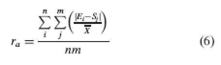
Step 1. To obtain a more accurate index of reciprocity, the first step is to average the height gaps (stigma–anther distances) of all possible crosses at each level in the population, instead of comparing the average heights for each sex at each level:

6

where r_a is mean relative reciprocity at level a, and X, average of heights of all organs (stigmas and stamens) in the population (to avoid over-representation of stamens, this value is calculated as the average of the stamens mean and the stigmas mean).

Note that the absolute value of the difference between E_i and S_j value is used, so the index will assess the average height gap independently of the sign of each individual gap. The denominator of the index of Richards and Koptur (1993) is replaced by a value that is common to all the population; therefore the relative indices obtained can be meaningfully compared among levels within the population, unlike the original index of Richards and Koptur (1993). However, as in these authors' original index, the closer to zero, the greater the reciprocity is for each level. These partial results can be plotted on an x–y graph as for those of Richards and Koptur.

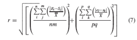
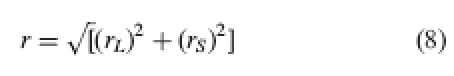
Step 2. A measure of overall reciprocity in a distylous population can be calculated as the Euclidian distance from zero of the population's location in the bivariate space defined by the two relative reciprocity indices:

7

or

8

where r is overall reciprocity of the population, r_L, relative reciprocity at level L, and r_S, relative reciprocity at level S.

The use of Euclidian distance is appropriate here because relative reciprocity indices at the two levels are comparable, as noted above.

Step 3. In a third step, the average standard deviation of the height gaps among organs at each level is included in the formula, so the final index is corrected by the dispersion of the data. The standard deviation at each level is calculated as follows:

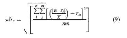9

where sdr_a is the standard deviation of the height gaps at level a.

Using the standard deviation of the height gaps instead of some absolute measure of dispersion of the organ lengths, prevents skew due to the greater abundance of stamens than stigmas. Given the standard deviations for each level, the average standard deviation is calculated as follows:

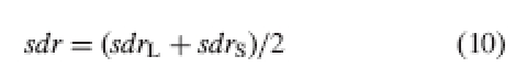10

where sdr_L is the standard deviation of height gaps at level L and sdr_S is the standard deviation of height gaps at level S.

Finally, the previous value from eqn (8) (r) is multiplied by the mean standard deviation (sdr) to calculate the final reciprocity value; the greater the dispersion of the data (sdr), the higher the value of the index (i.e. the lower the reciprocity). Thus, our final overall reciprocity index (R) for the population is:

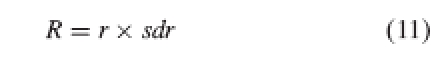11

where r is the reciprocity of the population as per eqn (8) and sdr is the mean standard deviation of height gaps, as per eqn (10).

With perfect reciprocity (i.e. all L-level stigmas and L-level stamens at exact same height, and all S-level stigmas and S-level stamens likewise at exactly same height), the value of the index is zero. Values depart from zero when reciprocity is not perfect, and are modulated by the average standard deviation of height gaps, so the greater the dispersion, the greater the departure from zero.

Testing the index: hypothetical cases

To test the behaviour of our reciprocity index, some hypothetical populations (see Materials and Methods) were constructed. Different situations were simulated, pre-specifying different means and standard deviations of stigma_L, stamen_L, stigma_S and stamen_S height, and then calculating the reciprocity index. For comparison, the index of Eckert and Barrett (1994) (after eqns 1 and 2) was also calculated using the same data. This index was chosen for comparison (a) because it has been the most widely used in previous studies of heterostyly, and (b) because it gives a single population value (unlike Richards and Koptur's index, with which our index cannot be compared). Nonetheless, note that these authors consider precision separately, so that the two indices are expected to perform differently.

Specifically, the indices were tested in the following simulated situations.

Case 1. This case was for comparison of five populations, all with equal mean heights of stigma_L and stamen_L, stigma_S and stamen_S, but with different levels of dispersion (Fig. 1).

Fig. 1.

(A) Values of the proposed index (closed circles) and Eckert and Barrett's index (squares) of reciprocity for five hypothetical populations with increasing dispersion of the data (for those of Eckert and Barrett: closed squares, unmodified index from mean values after eqn 1; open squares, modified values considering pairwise comparisons after eqn 2; see text). (B) Scatterplots of stigma (open circles) and anther heights (closed circles) of the five populations [mean stigmaL, stamenL, stigmaS and stamenS heights the same in all populations; and in all populations mean stigmaL = mean stamenL and mean stigmaS = mean stamenS; standard deviations (within each subgroup) 0·5, 1·0, 1·5, 2·0 and 2·5, respectively].

Since our index includes data dispersion in its formulation, it is evidently able to detect differences in dispersion, while the index of Eckert and Barrett (1994) cannot. When dispersion is the only variable modified, the increase in our index seems to be moderate when compared with other sources of variation (see next situation).

Case 2. Next the indices as applied to another five hypothetical populations were compared, this time with the same standard deviations but different mean height-gap patterns, ranging from heterostyly to stylar dimorphism (Fig. 2).

Fig. 2.

(A) Representation of the values of the indices of reciprocity for five hypothetical populations with increasing mean style–stigma distance in both morphs (symbols as for Fig. 1). (B) Scatterplots of stigma (open circles) and anther heights (closed circles) in the five populations. The difference between mean stigma height and mean stamen height (in each subgroup) increases from the left (gaps 0, 2, 4, 4, 6, respectively; see text for an explanation of population 4); standard deviation is 1·5 in all subgroups.

In this population series, both indices are sensitive to the increase in mean height gaps (stigma_L–stamen_L and stigma_S–stamen_S) as long as the gaps at the two levels are equivalent, i.e. while the stigma-over-stamen difference at one level is the same as the stamen-over-stigma difference at the other level. However, when anthers are above stigmas at both levels (as in hypothetical population 4 in Fig. 2), or vice versa (not shown), the index of Eckert and Barrett (1994) is unable to detect the lack of reciprocity, since it compares inter-organ distances rather than true reciprocity. This is especially clear when computed from pairwise comparisons after Formula 2. Some instances of this behaviour in heterostylous populations have, in fact, been found by Richards and Koptur (1993) (e.g. in Guettarda scabra, Palicourea fendleri and Palicourea petiolaris), and it has been seen in some populations of Lithodora diffusa.

Case 3. The indices were compared as applied to four hypothetical populations with the same standard deviations and the same mean height gap at one level, but different mean height gaps at the other level (Fig. 3).

Fig. 3.

(A) Representation of the indices of reciprocity for four hypothetical populations with increasing mean style–stigma distance in just one morph (symbols as for Fig.1). (B) Scatterplots of stigma (open circles) and anther heights (closed circles) in the four populations. The difference between mean stigmaL height and mean stamenL height is the same in all four populations, but the difference between mean stigmaS height and mean stamenS height increases from the left (0, 2, 4 and 6 in populations 1–4, respectively). The standard deviation is 1·5 in all subgroups.

In this population series both indices detect the increase in height gap at one level only, with reciprocity values about half of those obtained for populations with equivalent-magnitude height gaps at both levels (compare Figs 2 and 3). Notice that the unmodified index of Eckert and Barrett (1994) (from mean values, after Formula 1) detects poorly the decrease of reciprocity.

Finally, to get a general pattern of the variation of the index when varying mean stigma–stamen distances and the dispersion of the single data around those means, 70 hypothetical populations with increasing mean height gaps and standard deviations were constructed. The results can be plotted as a two-dimensional space of decreasing reciprocity (Fig. 4). It is important to stress that both factors (mean height distance and dispersion) contribute similarly to the final value of the index [regression standardized coefficients 0·65 and 0·69 for mean height distance and dispersion (sd), respectively; r² = 0·9, P < 0·001].

Fig. 4.

Two-dimensional space defined by the values on the index proposed, varying according to different mean stigma and stamen distances and different dispersion values (Sd). Small irregularities of the topography are due to the random origination of data.

Testing the index on natural populations of Lithodora

The species of the genus Lithodora vary between style dimorphic (L. prostrata and L. fruticosa) and distylous (L. oleifolia, L. diffusa or L. moroccana) (Fig. 5). In both cases, there is also considerable variability in the dispersion of both stamen (L. prostrata or L. oleifolia at Sant Aniol) and style heights (L. oleifolia at Sant Aniol). The cases selected here reflect a number of the situations proposed in the hypothetical examples. There is a clear difference between distylous and dimorphic populations for both indices, with values constantly under 0·05 (our index) or above 0·5 (Eckert and Barrett's index). Within those groups the indices clearly diverge. For the distylous populations the following differences were noted. (a) Between the two populations of L. oleifolia, the most reciprocal population according to the index of Eckert and Barrett (1994) is L. oleifolia at Sant Aniol, while for our index it is not. Considering the height distribution of stamens and stigmas in that population (Fig. 5B), the reciprocity cannot be higher than L. oleifolia at Monars: height distribution of stigmas is continuous in Sant Aniol, while clearly dimorphic in Monars; moreover, the dispersion of stamens as well as of stigmas is lower (more precise) in Monars. (b) The value of the index of Eckert and Barrett (1994) for L. diffusa is higher (more reciprocal) than that of L. moroccana or L. oleifolia at Monars. This is clearly an overestimation of that index for the same reason already mentioned for hypothetical population no. 4 in Fig. 2, i.e. in this population mean anther height is consistently higher than the mean of their target stigmas (organ level L: mean stigma height 9·98 mm, mean anther height 10·06 mm; organ level S: mean stigma height 5·70 mm; mean anther height 7·06 mm).

Fig. 5.

(A) Representation of the indices of reciprocity for six natural populations of different species of the genus Lithodora, arranged by increasing values of our index of reciprocity (symbols as for Fig. 1). (B) Scatterplots of stigma (open circles) and anther heights (closed circles) in the six populations. Populations of L. oleifolia correspond to Sant Aniol (L. oleifolia SA) and Monars (L. oleifolia MO) (see Materials and methods).

As for the dimorphic populations, L. prostrata is less reciprocal than L. fruticosa according to the index proposed here, but not for Eckert and Barrett's. This is an obvious consequence of considering the dispersion of the data (our index) or not (Eckert and Barrett 1994) (Fig. 5B).

CONCLUSIONS

The index of reciprocity presented here has several advantages over existing indices, which result in a more accurate characterization of reciprocity both in hypothetical populations and in real ones. First, it compares stigma–stamen height gaps for all potential crosses in the population, rather than simply mean values, avoiding the problems arising when means are used to represent populations with skewed distributions and/or outliers. Secondly, it comprises both stigma–stamen height distance at each level and precision (i.e. dispersion of the data in the population) in a single value that can be easily compared among populations or species, and that can also be correlated with fitness variables (see Hodgins and Barrett, 2006). Thirdly, it considers real reciprocity as opposed to equality of inter-organ levels. Fourthly, since the raw data are one-to-one organ comparisons, the index is not skewed by the more frequent sex. Fifthly, by using the same denominator for quantifying height gap at each level, the relative reciprocity indices obtained for each level can be meaningfully compared among populations and species.

The first three points are especially interesting, since marked within-population and even within-flower variation in stamen height at anthesis have been observed in some style polymorphic populations of the genera Lithodora, Narcissus and Nivenia, implying that reciprocity needs to be assessed at the population level; so considering a single value as representative of stamen length can be misleading. Thus, it is important to consider individual comparisons instead of means, and also to consider the dispersion of height-gap values, which in our view is often greater than is widely considered. Our index satisfies these criteria; since it includes data dispersion in its calculation, greater dispersion leads to higher values of the index (indicative of lower reciprocity), as shown in Fig. 1.

One minor objection that can be posed to our index is that it integrates ‘reciprocity’ and ‘precision’ (sensu Eckert and Barrett, 1994), which could lead to any loss of information on the individual behaviour of these variables. In our opinion, this possible drawback is greatly compensated by the prospect of being able to easily compare populations and species with a single value. One of the main possible applications of this index is to be related to phylogenetical reconstructions to study the evolution of heterostyly. As an example, some populations of the genus Lithodora have been used, obtaining an ordination of them according to reciprocity: when a phylogeny is available, the conclusions on the evolution of the polymorphism would vary greatly depending on the measure of reciprocity selected.

LITERATURE CITED

- Armbruster WS, Perez-Barrales R, Arroyo J, Edwards ME, Vargas P. Three-dimensional reciprocity of floral morphs in wild flax (Linum suffruticosum): a new twist on heterostyly. New Phytologist. 2006;171:581–590. doi: 10.1111/j.1469-8137.2006.01749.x. [DOI] [PubMed] [Google Scholar]
- Arroyo J, Barrett SCH, Hidalgo R, Cole W. Evolutionary maintenance of stigma-height dimorphism in Narcissus papyraceus (Amaryllidaceae) American Journal of Botany. 2002;89:1242–1249. doi: 10.3732/ajb.89.8.1242. [DOI] [PubMed] [Google Scholar]
- Baker A, Thompson JD, Barrett SCH. Evolution and maintenance of stigma-height dimorphism in Narcissus. II. Fitness comparisons between style morphs. Heredity. 2000;84:516–526. doi: 10.1046/j.1365-2540.2000.00686.x. [DOI] [PubMed] [Google Scholar]
- Baker HG. The evolution, functioning and breakdown of heteromorphic incompatibility systems. I. The Plumbaginaceae. Evolution. 1966;20:349–368. doi: 10.1111/j.1558-5646.1966.tb03371.x. [DOI] [PubMed] [Google Scholar]
- Barrett SCH. The evolution and adaptive significance of heterostyly. Trends in Ecology and Evolution. 1990;5:144–148. doi: 10.1016/0169-5347(90)90220-8. [DOI] [PubMed] [Google Scholar]
- Barrett SCH. Evolution and function of heterostyly. Berlin: Springer-Verlag; 1992. [Google Scholar]
- Barrett SCH. The evolution of plant sexual diversity. Nature Genetics. 2002;2:274–284. doi: 10.1038/nrg776. [DOI] [PubMed] [Google Scholar]
- Barrett SCH, Hodgins KA. Floral design and the evolution of asymmetrical mating. In: Harder LD, Barrett SCH, editors. The ecology and evolution of flowers. Oxford: Oxford University Press; 2006. pp. 239–255. [Google Scholar]
- Charlesworth D, Charlesworth B. A model for the evolution of distyly. American Naturalist. 1979;114:467–498. [Google Scholar]
- Darwin C. The different forms of flowers on plants of the same species. London: John Murray; 1877. [Google Scholar]
- Dulberger R. Floral polymorphisms and their functional significance in the heterostylous syndrome. In: Barrett SCH, editor. Evolution and function of heterostyly. Berlin: Springer-Verlag; 1992. pp. 41–84. [Google Scholar]
- Eckert CG, Barrett SCH. Tristyly, self-compatibility and floral variation in Decodon verticillatus (Lithraceae) Biological Journal of the Linnean Society. 1994;53:1–30. [Google Scholar]
- Eckert CG, Mavraganis K. Evolutionary consequences of extensive morph loss in tristylous Decodon verticillatus (Lythraceae): a shift from tristyly to distyly? American Journal of Botany. 1996;83:1024–1032. [Google Scholar]
- Ganders FR. The biology of heterostyly. New Zealand Journal of Botany. 1979;17:607–635. [Google Scholar]
- Hildebrand F. Experimente über den dimorphismus von Linum perenne und Primula sinensis. Botanische Zeitung. 1864;22:1–5. [Google Scholar]
- Hodgins KA, Barrett SCH. Female reproductive success and the evolution of mating type frequencies in tristylous populations. New Phytologist. 2006;171:569–580. doi: 10.1111/j.1469-8137.2006.01800.x. [DOI] [PubMed] [Google Scholar]
- Lau P, Bosque C. Pollen flow in the distylous Palicourea fendleri (Rubiaceae): an experimental test of the disassortative pollen flow hypothesis. Oecologia. 2003;135:593–600. doi: 10.1007/s00442-003-1216-5. [DOI] [PubMed] [Google Scholar]
- Lewis D, Rao AN. Evolution of dimorphism and population polymorphism in Pemphis acidula. Proceedings of the Royal Society of London, Series B. 1971;178:79–94. [Google Scholar]
- Lloyd DG, Webb CJ. The evolution of heterostyly. In: Barrett SCH, editor. Evolution and function of heterostyly. Berlin: Springer-Verlag; 1992. pp. 151–178. [Google Scholar]
- Lloyd DG, Webb CJ. The selection of heterostyly. In: Barrett SCH, editor. Evolution and function of heterostyly. Berlin: Springer-Verlag; 1992. pp. 179–207. [Google Scholar]
- Lloyd DG, Webb CJ, Dulberger R. Heterostyly in species of Narcissus (Amaryllidaceae) and Hugonia (Linaceae) and other disputed cases. Plant Systematics and Evolution. 1990;172:215–227. [Google Scholar]
- Massinga PH, Johnson SD, Harder LD. Heteromorphic incompatibility and efficiency of pollination in two distylous Pentanisia species (Rubiaceae) Annals of Botany. 2005;95:389–399. doi: 10.1093/aob/mci040. [DOI] [PMC free article] [PubMed] [Google Scholar]
- Pérez R, Arroyo J, Armbruster WS. Differences in pollinator faunas may generate geographic differences in floral morphology and integration in Narcissus papyraceus (Amaryllidaceae) Oikos. 2007;116:1904–1918. [Google Scholar]
- Richards AJ. Lethal linkage and its role in the evolution of plant breeding systems. In: Owens SJ, Rudall PJ, editors. Reproductive biology. London: Royal Botanic Gardens, Kew; 1998. pp. 71–83. [Google Scholar]
- Richards JH, Koptur S. Floral variation and distyly in Guetarda scabra (Rubiaceae) American Journal of Botany. 1993;80:31–40. [Google Scholar]
- Thompson JD, Pailler T, Strasberg D, Manicacci D. Tristyly in the endangered Mascarene Island endemic Hugonia serrata (Linaceae) American Journal of Botany. 1996;83:1160–1167. [Google Scholar]
- Thompson JD, Barrett SCH, Baker AM. Frequency-dependent variation in reproductive success in Narcissus: implications for the maintenance of stigma-height dimorphism. Proceedings of the Royal Society. 2003;270:949–953. doi: 10.1098/rspb.2002.2318. [DOI] [PMC free article] [PubMed] [Google Scholar]
- Weller SG. Evolutionary modifications to tristylous breeding systems. In: Barrett SCH, editor. Evolution and function of heterostyly. Berlin: Springer-Verlag; 1992. pp. 247–272. [Google Scholar]