

Abstract
Longitudinal relaxation of brain water 1H magnetization in mammalian brain in vivo is typically analyzed on a per voxel basis using a monoexponential model, thereby assigning a single relaxation time constant to all 1H magnetization within a given voxel. This approach was tested by obtaining inversion recovery data from grey matter of rats at 64 exponentially-spaced recovery times. Using Bayesian probability for model selection, brain water data were best represented by a biexponential function characterized by fast and slow relaxation components. At 4.7 T, the amplitude fraction of the rapidly relaxing component is 3.4 ± 0.7 % with a rate constant of 44 ± 12 s-1 (mean ± SD; 174 voxels from 4 rats). The rate constant of the slow relaxing component is 0.66 ± 0.04 s-1. At 11.7 T, the corresponding values are 6.9 ± 0.9 %, 19 ± 5 s-1, and 0.48 ± 0.02 s-1 (151 voxels from 4 rats). Several putative mechanisms for biexponential relaxation behavior were evaluated, and magnetization transfer between bulk water protons and non-aqueous protons was determined to be the source of biexponential longitudinal relaxation. MR methods requiring accurate quantification of longitudinal relaxation may need to take this effect explicitly into account.
Keywords: magnetization transfer, inversion recovery, rat brain, chemical exchange, Bayesian probability
Introduction
Longitudinal relaxation rate constant (R1 = 1/T1) measurements of tissue water are key to a variety of MR methods, including dynamic contrast enhanced techniques (1) and assessment of multiple sclerosis patients for damage to normal appearing white matter (2). Data from such measurements in brain are typically modeled as a monoexponential magnetization recovery, assuming that the longitudinal relaxation of all water can be represented by a single R1. However, in vivo voxel resolution is coarse on the scale of tissue microstructure and water exists in a variety of magnetic environments (“compartments”) within a single in vivo voxel. Each compartment potentially provides a unique relaxation environment for water. Consistent with this concept, a variety of tissues display multiexponential T2 relaxation and each exponential component can be assigned to a unique anatomical compartment (3,4). Further, multiple R1 components have been described for peripheral nerve (4,5), though not for brain gray matter.
Non-monoexponential in vivo relaxation data are generally analyzed by one of two methods. The first method models relaxation data as the sum of a small number of discrete exponential functions, with each exponential component having a unique amplitude and R1. In this case, the implicit biophysical picture is that water within a given voxel can be approximated as residing in a few separate magnetic environments that are not in fast exchange. In the limit of slow exchange this would enable measurement of compartment specific R1 values. The second method models relaxation data with a continuous distribution of exponential functions. Here the implicit biophysical picture is that water within a given voxel should be approximated as residing in a large number of separate magnetic environments that are not in fast exchange (6,7).
Taking advantage of high field magnets equipped with high performance gradients, the study reported herein was done using highly time resolved inversion recovery (IR) spin-echo, echo-planar imaging (SEPI) to acquire data sets with 64 to 128 exponentially spaced inversion time (TI) values. Bayesian probability theory (8,9) was employed to select among models composed of sums of from one to four exponentials. The relaxation data were best characterized by biexponential recovery for essentially all in vivo rat brain voxels.
Aside from pulse sequence and scanner induced artifacts, four mechanisms were considered to explain this non-monoexponential IR relaxation behavior: blood flow, radiation damping, multiple non-exchanging magnetic environments (“compartments”), and a special case of multiple compartments - magnetization transfer (MT). The source of biexponential longitudinal relaxation behavior was the MT phenomenon. It was possible to image MT via measurement of longitudinal relaxation without application of an off-resonance pulse as normally used to generate MT image contrast. These results bear directly on the quantitative analysis of longitudinal relaxation based MRI methods.
Magnetization Transfer
Magnetization transfer can occur either by direct chemical exchange or by indirect dipole-mediated cross relaxation. Both mechanisms are described by an analogous set of coupled differential equations (10). A concise summary of the relevant mathematical formalism describing two-site magnetization transfer is provided in the Appendix. For convenience, the equations and terminology for chemical exchange are employed. It follows from this mathematical analysis that the observed two-site time-dependent magnetization, either with or without off-resonance radio frequency (rf) saturation of the non-aqueous 1H, is appropriately modeled as a monoexponential plus a constant or a biexponential plus a constant, respectively. Throughout this manuscript, the presence of the constant will be assumed and the signal model will be described simply as the number of exponentials (i.e., monoexponential or biexponential).
Methods
Phantom Preparation for Control MR Analysis
Crosslinked 15% bovine serum albumin (BSA) was prepared as described previously (11). Briefly, a 30% “essentially fatty acid free” BSA solution (Sigma Aldrich, St Louis, MO) was diluted to 15% using phosphate-buffered saline (PBS, pH 7.4) and placed on ice for 10 minutes. Then, 25 μL/mL of an ice cold 50% glutaraldehyde solution (Electron Microscopy Sciences, Hatfield, PA) were added to the BSA solution. This solution was mixed, left on ice for 30 minutes, and then kept at room temperature for an additional 2 hours before being stored at 4°C.
Tissue Preparation for ex Vivo MR Analysis
A rat (n = 1) was perfused through the left cardiac ventricle with ice cold PBS (pH 7.4) followed by 4% paraformaldehyde in PBS (pH 7.4). The brain was dissected prior to overnight immersion in 4% paraformaldehyde and then transferred to PBS for storage at 4°C.
Animal Preparation for in Vivo MR Analysis
All experimental procedures were performed in accordance with NIH guidelines and Washington University Institutional Animal Care and Use Committee regulations. Male Sprague–Dawley rats weighing 329 ± 36 g (mean ± standard deviation) were anesthetized with isoflurane (3% in O2) followed by intraperitoneal injection of a 10% urethane solution (0.6 mL per 100 g body weight). Identical injections of the same solution were administered 5 and 30 min after the initial injection for a total anesthetic dose of 1.8 g/kg.
A MR-compliant head holder consisting of ear bars and a nose cone/bite bar was used to minimize animal motion. Heart rate and arterial oxygenation were monitored with a pulse oximeter and a fiber optic sensor (Nonin Medical, Plymouth, MN) attached to a hind paw. Blood oxygenation levels were maintained by supplying 100% O2 gas through the nose cone. Body core temperature was monitored rectally with a fiber optic temperature probe (FISO, Québec, Canada) and maintained at 37 ± 1 °C using circulating warm water. To assess the influence of blood flow in the R1 measurement, one rat was sacrificed in the magnet by administration of 1 mL of 2 M KCl via a tail vein catheter.
Scanner and Pulse Sequence Attributes for in Vivo MR Analysis
Imaging and spectroscopy experiments employed one of two MR systems. The first is built around an Oxford Instruments (Oxford, U.K.) 4.7 T magnet (40 cm diameter, clear bore) equipped with 10 cm inner diameter, actively shielded Magnex Scientific (Oxford, U.K.) gradient coils capable of producing magnetic field gradients up to 60 G/cm. The second is built around a Magnex Scientific 11.7 T magnet (26 cm diameter, clear bore) equipped with 8 cm inner diameter, actively shielded Magnex Scientific gradient coils capable of producing magnetic field gradients up to 120 G/cm. Varian (Palo Alto, CA) UNITYINOVA consoles control both magnet/gradient systems. Data were collected at 4.7 T using a 3.8 cm inner diameter Litzcage coil (Doty Scientific, Columbia, SC) or either a 1.5 or 2.5 cm inner diameter birdcage coil (Stark Contrast, Erlanger, Germany). Data were collected at 11.7 T using a 4 cm inner diameter birdcage coil (Stark Contrast). Multi-slice gradient-echo data were collected to identify the transverse slice used for subsequent SEPI data collection. Once a slice was identified, manual shimming was performed on the slice using the LASER pulse sequence (12).
The SEPI acquisition parameters, unless otherwise noted, were: repetition time (TR) ∼ 5 (vide infra), spin echo time (TE) 56 ms (4.7 T) or 34 ms (11.7 T), bandwidth of 100 kHz (4.7 T) or 400 kHz (11.7 T), one signal average to collect all k-space lines for an image, slice thickness 2 mm, field of view 4 × 4 cm, data matrix 64 × 64. Two separate pulse sequences were used to collect IR data. In the first, standard IR data, using 64 exponentially spaced TI values from 4 ms to 6 s, were collected using a SEPI sequence that was preceded by a nonselective square inversion rf pulse (to minimize blood inflow effects). Crusher gradients (1 ms) were applied on all three axes during TI to suppress any residual transverse magnetization arising from an imperfect inversion pulse. In the second sequence, off-resonance saturation, using square rf pulses, was incorporated into the IR pulse sequence (MT-IR) during the preacquisition and TI delays. The off-resonance rf was applied at +20 kHz with respect to water (0 Hz) with an average bandwidth of approximately 680 Hz, as determined from the length of time required by a square rf pulse at the same power amplifier output to invert the equilibrium magnetization (13). The time constant (Tss) characterizing the time evolution of bulk water magnetization to a partially-saturated steady-state in the presence of off-resonance rf irradiation was determined by a SEPI pulse sequence that was preceded by a varying length MT pulse (16 exponentially spaced MT pulse lengths from 0.1 to 10 s applied at +20 kHz).
The image with the longest TI value from each sequence was used as the anatomic reference image.
MR Data Analysis
Absorption mode images were calculated using one zero-order and two first-order phase parameters estimated using Bayesian probability theory. All images were thresholded so that any voxel in the anatomic reference image with signal less than five times the estimated noise standard deviation was set to zero. Bayesian probability theory and Markov chain Monte Carlo integration were used for exponential model selection and parameter estimation (8,9) on a per voxel basis. The signal model for each voxel in either an IR or IR-MT data set was selected from the following family of models: (i) no signal, (ii) a constant offset, (iii) from one to four exponentials (either with or without a constant). The posterior probability for each model was determined and the most probable model selected. Similarly, the most probable value of each parameter defining the selected model (e.g., component rate constants and amplitudes) was taken as the optimal parameter estimate.
For biexponential analysis, IR data were modeled as the sum of two exponentials plus a constant:
| [1] |
where A and B are the amplitudes of the two exponentials, is the smaller exponential rate constant, is the larger exponential rate constant, and C is a constant that represents the equilibrium value for the longitudinal magnetization. The amplitude fraction of the fast relaxing component (f+) was defined as Y/(X + Y) and the amplitude fraction of the slow relaxing component (f−) was defined as X/(X + Y), which is equivalent to 1 - f+. Bayesian model selection maps, which display the most appropriate model for each voxel, were thresholded by setting voxels modeled as monoexponential to gray, voxels modeled as biexponential to white, and all other voxels to black.
Data acquired by a SEPI sequence preceded by a varying length MT pulse were modeled with a monoexponential function (13) and an ROI from the brain was used to estimate Tss. The prepulse in the MT-IR sequence was set to approximately 10 × Tss to ensure a steady-state saturation level was achieved.
Results
Model Selection and Parameter Estimation
Representative in vivo single voxel IR data from rat brain are shown in Fig. 1. In this example, 128 exponentially spaced TI values were used to sample the IR time course. The inset shows the residuals when the data are modeled with either a monoexponential or a biexponential function. Since the noise in a pure absorption mode image is uncorrelated with a zero mean Gaussian distribution, the residuals are expected to fluctuate around zero. The systematic trend evident in the residuals when the data are modeled with a monoexponential function indicates that the model does not fit the data to the noise level. The residuals for a biexponential model are randomly distributed around zero, which is qualitative evidence that the data are better modeled – indeed, modeled to the noise level – with a biexponential function.
Figure 1.
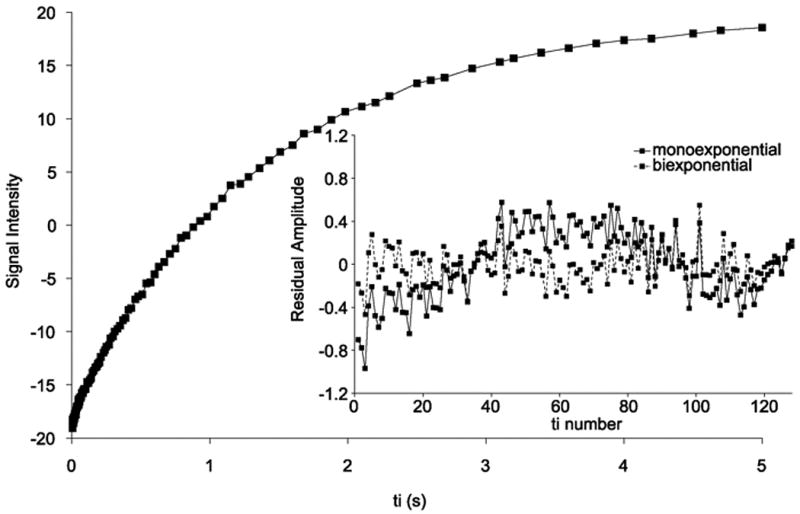
In vivo, 4.7 T single voxel IR data from rat brain collected using 128 exponentially spaced TI values from 5 ms to 5 s and 2 signal averages. The inset shows the residual amplitudes from fitting the data to either a monoexponential (solid line) or a biexponential function (dashed line).
Figure 2A shows an anatomic reference image. The main features in this image are the rat brain and a tube resting on top of the head containing 0.1 mM Omniscan™. The most probable model within a family of exponential models was determined on a per voxel basis using Bayesian probability theory. The map shown in Fig. 2B summarizes this model selection calculation; gray voxels are modeled as a monoexponential, white voxels are modeled as a biexponential, all other voxels are colored black. The 0.1 mM Omniscan™ is best modeled as a monoexponential and the rat brain has a ubiquitous distribution of biexponential voxels. Examination of other rats and an in vivo LASER localized voxel (2 × 2 × 2 mm) in the striatum showed this to be a consistent finding. Relaxation models consisting of sums of three or four exponential components had near zero probability for all voxels and are not considered further.
Figure 2.
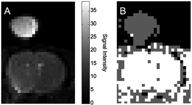
Expanded region from an IR data set at 4.7 T. A) Anatomic reference image showing the rat brain and a 0.1 mM Omniscan™ phantom. B) Bayesian model selection map. The in vivo rat brain data is best modeled with a biexponential function (white voxels) and the aqueous Omniscan™ phantom data is best modeled with a monoexponential function (gray voxels).
In vivo IR data (64 exponentially spaced TI times, data matrix 64 × 64) were acquired from four different rats at 4.7 T and at 11.7 T and modeled with a biexponential function. Using voxels from the striatum, the biexponential decay rate constants ( and ) and amplitude fraction f+ were estimated and are summarized in Table 1.
Table 1. In vivo rat brain Bayesian parameter estimatesa.
| Field strength: | 4.7 T | 11.7 T | |
|---|---|---|---|
| Sequence: | IR | IR-MT | IR |
| (s-1): | 44 ± 12 | 1.4 ± 0.1 | 19 ± 5 |
| (s-1): | 0.66 ± 0.04 | 0.48 ± 0.02 | |
| f+ (%): | 3.4 ± 0.7 | 6.9 ± 0.9 | |
data are mean ± standard deviation (n = 4)
Testing the Putative Origins for the Observed Biexponential Longitudinal Relaxation
Pulse Sequence or Scanner Artifacts
Using the pulse sequences described herein, monoexponential – not biexponential – relaxation was observed in dilute aqueous solutions that served as phantoms. Further, maps of the biexponential component amplitudes delineate known anatomy. To illustrate this, a higher spatial resolution IR data set (n =1; data matrix 128 × 128) was collected at 11.7 T and modeled with a biexponential function. The f+ parametric map (Fig. 3) clearly displays white matter structures (corpus callosum and external capsule) with a larger amplitude fraction (9.4 ± 1.6 %) than gray matter (6.8 ± 0.8 %).
Figure 3.
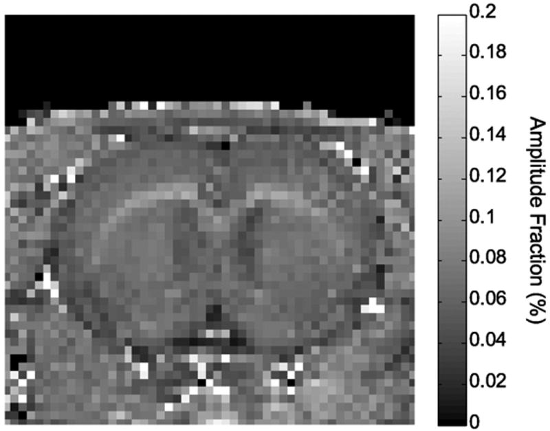
Parametric map of the amplitude fraction for the fast relaxing component (f+) obtained at 11.7 T. The image is an enlarged region from an image collected with a data matrix of 128 × 128. Anatomic structures are visible and white matter (corpus callosum and external capsule) has a larger amplitude fraction than gray matter.
Blood Flow Artifacts
A nonselective inversion pulse was used to minimize artifacts from blood flowing through the imaging slice (14). Nevertheless, f+ is in the range typical for mammalian intravascular volume (15-17) suggesting that inflow of blood may be responsible for the rapid relaxation component. To test for this artifact, in vivo IR data at 4.7 T were collected (n = 1) before and immediately following an intravascular KCl injection (i.e., zero blood flow). Striatal voxels were biexponential both with blood flow (f+ = 3.7 ± 0.8 %, , and ) and without flow (f+ = 4.6 ± 0.8 %, , and ). Blood, whether flowing or stationary, may have a paramagnetic contribution from the iron centers in hemoglobin. Therefore, an ex vivo paraformaldehyde perfusion-fixed (bloodless) room-temperature rat brain (n = 1) was imaged at 4.7 T. The anatomic reference image is shown in Fig. 4A, and the Bayesian model selection map is shown in Figure 4B. As expected, relaxation data from the PBS buffer surrounding the excised brain are best modeled with a monoexponential function. However, relaxation data from the fixed tissue are predominantly best modeled with a biexponential function. The biexponential parameter estimates for striatal voxels are: f+ = 9 ± 2 %, , and .
Figure 4.
Ex vivo fixed rat brain at 4.7 T collected at room-temperature with a 4 segment IR-SEPI. A) Anatomic reference image. B) Bayesian model selection map. The ex vivo rat brain data are best modeled as two exponentials plus a constant (white voxels) and the PBS buffer data are best modeled as one exponential plus a constant (gray voxels).
Radiation Damping Artifacts
Coupling between the transverse magnetization and rf coil can cause radiation damping (18-20), resulting in biexponential longitudinal relaxation. The radiation damping rate constant is proportional to the bulk magnetization and coil filling factor. To test for this artifact, relaxation data were collected at 4.7 T (n = 1) and 11.7 T (n = 1) using experimental parameters identical to those used for in vivo imaging on a large 0.1 mM Omniscan™ phantom, which provided a larger bulk magnetization and coil filling factor than a rat. Voxels from the phantom were best modeled with a monoexponential – not a biexponential – function (data not shown).
Two Non-Exchanging Compartments
The amplitude fraction of the rapidly relaxing component for non-exchanging or slowly exchanging systems should increase as TR is reduced, a result of progressive saturation of the slowly relaxing component (21). To test for this situation, in vivo relaxation data sets were collected at 4.7 T (n = 1) and 11.7 T (n = 1) using two different TR values. A long TR value (8 s at 4.7 T or 11 s at 11.7 T), which allowed full longitudinal recovery, and a short, partially saturating, TR value (0.5 s) were used at both field strengths. The data acquired with a TR of 0.5 s were obtained with eight signal averages, preceded by eight pulses to reach steady-state. TR values of 8 s and 0.5 s were used at 4.7 T. The data from striatial voxels using a TR of 8 s were best modeled as biexponential relaxation where f+ = 3.7 ± 0.6 %. The TR = 0.5 s data were best modeled as slow monoexponential relaxation, i.e., f+ = 0. To confirm the decrease in f+ at short TR, higher signal-to-noise relaxation data were obtained at 11.7 T (n = 1). Comparing data with TR of 11 s and 0.5 s, relaxation was best modeled as biexponential and f+ decreased from 8 ± 2 % to 2.6 ± 0.7 %, respectively.
Magnetization Transfer
Magnetization transfer from either chemical exchange or dipole mediated cross relaxation can cause non-monoexponential relaxation. Crosslinked BSA phantoms are known to exhibit magnetization transfer effects (11,22). Data were collected at 4.7 T on a 0.1 mM Omniscan™ phantom and a crosslinked 15% BSA phantom. Figure 5A shows the Bayesian model selection map for samples of 0.1 mM Omniscan™ (upper left) and crosslinked 15% BSA (bottom right) using the IR pulse sequence (absence of off-resonance rf irradiation). Figure 5B shows the corresponding Bayesian model selection map using an MT-IR pulse sequence (presence of off-resonance rf irradiation). Data from the Omniscan™ phantom are best modeled with a monoexponential function in both cases (IR: 0.835 ± 0.003 s-1, MT-IR: 0.830 ± 0.003 s-1). As expected, data collected from the crosslinked 15% BSA phantom are best modeled with a biexponential function in the absence of the MT pulse (f+ = 7.3 ± 0.5 %, , and ) and a monoxponential function in the presence of the MT pulse (R1 = 3.22 ± 0.07 s-1).
Figure 5.
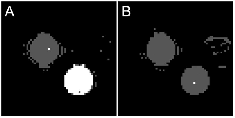
Effect of off-resonance saturation on phantoms at 4.7 T. A) Bayesian model selection map from data obtained without off-resonance saturation (IR data). B) Bayesian model selection map from data obtained with off-resonance saturation (MT-IR data). The 0.1 mM Omniscan™ phantom (upper left) data are best modeled with a monoexponential function (gray voxels) in both data sets. For the crosslinked 15% BSA phantom (bottom right), the IR data are best modeled with a biexponential function (white voxels) and the MT-IR data are best modeled as a monoexponetial function (gray voxels).
In a separate experiment, inversion recovery data at long and short TR were also collected on the crosslinked 15% BSA phantom at 4.7 T. When the TR is reduced from 8 s to 0.5 s, f+ decreased from 7.8 ± 0.1 % to 4.1 ± 0.1 %.
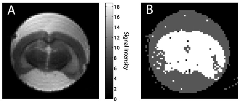
The MT-IR sequence was applied to in vivo rat brain (n = 4). A representative Bayesian model selection parametric map is shown in Fig. 6A. These data are from the same rat shown in Fig. 2. There is a marked reduction in the number of voxels best modeled by a biexponential function (white voxels) between Fig. 2B and Fig. 6A. Monoexponential rate constant (R1) maps are shown for both the MT-IR data (Fig. 6B) and IR data (Fig. 6C). In both cases, the data are fit to monoexponential functions, though the IR data from brain shown in panel C are actually best fit by a biexponential function. Note that in the presence of an off-resonance rf saturation pulse, there is a difference in R1 values between brain and muscle that is not apparent in the absence of the off-resonance pulse. The brain R1 is increased (IR modeled with a monoexponential function: 0.68 ± 0.4 s-1, MT-IR: 1.4 ± 0.1 s-1) when off-resonance saturation is applied (Table 1). The off-resonance pulse had no effect on the Omniscan™ R1 value (data not shown), and these data were best modeled with a monoexponential function both with and without the off-resonance pulse.
Figure 6.
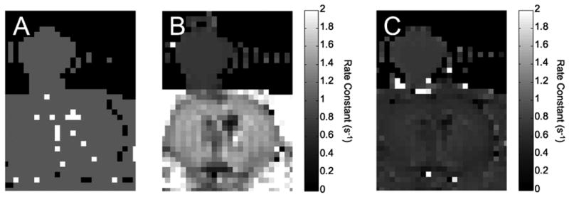
Effect of off-resonance saturation on in vivo rat brain at 4.7 T. A) Bayesian model selection map. The 0.1 mM Omniscan™ and rat brain data are best modeled with a monoexponential function (gray voxels). B) Parametric map, using four signal averages, of the MT-IR rate constant. The rate constant is higher for muscle than brain. C) Parametric map of the IR rate constant modeled as a monoexponential. The rate constants are similar between the brain and muscle.
Discussion
Due to experimental time constraints, longitudinal relaxation rate constants in vivo are often determined using a small number of TI values. Faster image acquisition methods such as EPI make it possible to collect 64 exponentially spaced TI values in an experimentally acceptable time (about 10 minutes). At both high signal-to-noise ratio and TI resolution, in vivo rat brain inversion recovery relaxation data can be modeled into the noise with a biexponential function, but not with a monoexponential function. Five possible etiologies for this biexponential behavior were evaluated: imperfections in pulse sequence and/or scanner performance, blood flow, radiation damping, the presence of two non-exchanging water compartments with different longitudinal relaxation rate constants, and magnetization transfer.
Artifacts due to pulse sequence or scanner performance shortcomings were ruled out by the absence of biexponential relaxation in homogeneous aqueous phantoms and by the clear definition of known anatomical structure in maps of, for example, f+, in experiments with rat brain in vivo. Data collection was designed to minimize effects from flowing blood by using a non-slice-selective inversion pulse (14). Nevertheless, artifacts due to blood flow effects were conclusively ruled out. Biexponential relaxation, similar in character to that observed in vivo, was observed with rat brain in situ immediately following sacrifice when there is no blood flow and with paraformaldehyde perfusion-fixed rat brain ex vivo when there is neither blood nor flow. Further, the contrast in a map of f+ (Fig. 3) would be reversed if f+ was dependent on blood volume, because gray matter has approximately twice the intravascular volume of white matter (23). Radiation damping, which typically requires high Q coils and high field strengths, is well known to cause artifacts in high-resolution solution-state NMR (24,25) and can cause biexponential longitudinal relaxation (26). In the presence of a receiver coil with Q depressed by a conducting sample such as tissue, radiation damping is unlikely, though there is evidence that it complicates MR blood flow measurements (27). Artifacts due to radiation damping were ruled out by experiments with homogeneous aqueous phantoms where purely monoexponential relaxation was observed.
The possibility of two non-exchanging compartments with different longitudinal relaxation rates was examined by performing the IR SEPI experiment at long and short TR. For two non-exchanging or slowly exchanging compartments, reducing TR should increase f+ (21). Relaxation experiments in vivo showed that f+ decreased with shortened TR, indicating a more complex relationship between the two exponential relaxation components, which is consistent with previous results (28) and will be discussed below. The final mechanism considered as a source of the observed biexponential relaxation was magnetization transfer. In its simplest form (Appendix), MT analysis assumes that tissue 1H content is composed of two components: non-aqueous 1H and bulk water 1H. In the presence of an off-resonance rf pulse, magnetic coupling between these two components, either by cross-relaxation or chemical exchange, allows the non-aqueous component to indirectly affect the bulk water component. Therefore, MT images reflect characteristics of the non-aqueous component.
Assuming the biexponential IR relaxation component with the larger rate constant (R+) predominantly reflects the rapid exchange (transfer) of near-thermal-equilibrium magnetization from the minimally perturbed non-aqueous 1H pool into the bulk water pool of inverted 1H magnetization, white matter would be expected to have a larger f+, as seen in Fig. 3, because white matter has a larger MT effect than gray matter (29). However, recall from the Appendix that the amplitude fractions f+ and f− estimated from the biexponential model, Eq. [1], are complex functions that depend not only on the true populations and field-dependent intrinsic relaxation rate constants of the two 1H pools, but also on the kinetic rate constants governing exchange between the two pools. Thus, while f+ and f− are accurately the biexponential component amplitude fractions, they are only apparent pool size fractions.
It was noted previously that decreasing TR reduces f+. Using Eq. [A-4a] and Eq. [A-4b] in the Appendix, the following equation is derived for the general form of f+:
| [2] |
where represents the longitudinal magnetization deviation from thermal equilibrium for bulk water 1H (A) or non-aqueous 1H (B). None of the parameters in Eq. [2] can have negative values and R+ > by definition. Therefore, the slope of f+ vs. ΔMB is negative at all TR values. This has important consequences.
In the idealized limit where the IR sequence is completely selective for bulk water 1H magnetization (the A site), ΔMB = 0 and f+ is a maximum. In practice, the broad non-aqueous 1H resonance is minimally affected by a low bandwidth rf inversion pulse and long TR. Thus, ΔMB is close to zero, and f+ is near maximal. The situation changes as TR becomes shorter. Recall, the long motional correlation times characterizing the non-aqueous matrix (minimal spectral density at ω0) result in a small intrinsic R1 for the non-aqueous 1H pool. Thus, a series of IR sequence repetitions separated by a short TR can significantly reduce the non-aqueous 1H longitudinal magnetization. This reduces and increases ΔMB, which leads to a decrease in f+ as observed experimentally herein.
This effect is exacerbated by modulating ΔMA. A long TR value and effective inversion of the narrow 1H resonance of the bulk water pool maximize ΔMA, resulting in a limiting slope and minimal dependence of f+ on changes in ΔMB. As TR is shortened and pulse sequence repetitions become more closely spaced, the 1H longitudinal magnetization of the bulk water pool is reduced (partially saturated), quickly reaching a steady-state level. Subsequent inversion of this steady-state magnetization yields a decreased ΔMA (from a reduced ), which increases the sensitivity of f+ to ΔMB.
The observed relaxation behavior in the presence of off-resonance rf saturation provides further evidence for MT as the source of the biexponential relaxation. As shown in the Appendix, biexponential relaxation will become monoexponential with saturation of the macromolecular longitudinal 1H magnetization. This can be accomplished with off-resonance rf irradiation. Assuming complete saturation of the non-aqueous longitudinal 1H magnetization (pool B) and no direct saturation of bulk water 1H magnetization (pool A), the rate constant describing the now monoexponential relaxation (R1) is predicted to be greater than that found for the “slow” biexponential component in the absence of saturating irradiation (30). This was, indeed, observed with rat brain in vivo at 4.7 T where R1 = 1.4 ± 0.1 and .
Crosslinked BSA phantoms are known to exhibit magnetization transfer effects (11,22) and, thus, provide a positive control. Consistent with expectations, the crosslinked BSA phantom relaxation was biexponential in the absence of off-resonance rf irradiation and monoxponential in the presence of off-resonance rf irradiation. Further, as predicted, the rate constant describing the monoexponential relaxation (R1 = 3.22 ± 0.07 s-1) was greater than that found for the slowly relaxing biexponential component in the absence of off-resonance rf irradiation .
It is worth emphasizing that, even though R1 is reproducible under a given set of experimental conditions, it is not a particularly quantitative parameter. This is because the magnetization transfer effect in the presence of off-resonance rf irradiation is a complex combination of pulse sequence and relaxation parameters (13,31).
Efforts have been made in previous MR studies to correlate relaxation rate constant changes with pathology (32,33). Unfortunately, relaxation rate constants were of limited clinical diagnostic utility (34). It is likely that by sampling only a limited number of TI values, previous studies only provided an estimate of the bulk water pool relaxation (i.e., ). Consistent with this expectation, the parameter estimates reported in Table 1 for at both 4.7 T and 11.7 T field strengths are similar to previous reports of longitudinal relaxation data modeled as monoexponential (35,36). The data presented here suggest that and f+ are more intimately associated with the non-aqueous matrix and would, therefore, possibly be a better diagnostic metric of pathology and treatment response. A benefit of pursuing IR methods and avoiding MT pulses would be a reduction in rf power deposition and concomitant tissue heating (37) when compared to conventional MT methods.
Conclusion
We have shown that in vivo rat brain inversion recovery data are best modeled as biexponential. To our knowledge, this is the first report of directly observed biexponential longitudinal relaxation in brain gray matter. The biophysical origin of this relaxation behavior is magnetization transfer between bulk water and non-aqueous 1H pools. These effects should be taken into account for MR methods that require highly-accurate measurements of brain water 1H longitudinal relaxation. Findings herein suggest that it is possible to directly image in vivo MT. This approach could potentially be used to diagnose and monitor treatment for diseases that involve macromolecular reorganization and associated changes in MT.
Acknowledgments
The authors would like to thank Dr. Joong Hee Kim for providing the perfusion-fixed brain. This research was funded by NIH grants EB002083 and R24-CA83060 (NCI Small-Animal Imaging Resource Program).
Appendix
Magnetization transfer can occur either by direct chemical exchange or by indirect dipole-mediated cross-relaxation. Both mechanisms are described by an analogous set of coupled differential equations (10). For convenience, the equations and terminology for chemical exchange are employed herein.
The Bloch equations for longitudinal magnetization as modified for two-site magnetization transfer via chemical exchange by McConnell are (38):
| [A-1a] |
| [A-1b] |
where and are the equilibrium longitudinal magnetizations in sites A and B, respectively, and k1A = kA + R1A and k1B = kB + R1B where R1A and R1B are the intrinsic longitudinal relaxation rate constants in the absence of exchange and kA and kB are the kinetic exchange rate constants for magnetization leaving the A and B sites, respectively. The Bloch-McConnell equations have the following general solution (39):
| [A-2a] |
| [A-2b] |
| [A-3a] |
| [A-3b] |
| [A-4a] |
| [A-4b] |
| [A-4c] |
| [A-4d] |
where MA(t) and MB(t) are the time-dependent signal intensities, and and are the initial intensities immediately following a perturbation. Typically, the “A” 1H-magnetization pool is assigned to bulk water and the “B” 1H-magnetization pool is assigned to the non-aqueous matrix (13), which has a short T2 (∼ 10 μs) and is thus invisible by normal solution-state MRI techniques. Therefore, even though the two pools or compartments have arguably the same chemical shift, the total observed 1H signal is MA(t), and the actual observed time-dependent signal intensity is functionally biexponential (Eq. [A-2a]).
When the non-aqueous 1H magnetization of compartment B is selectively and completely saturated with an off-resonance rf pulse, the observed time-dependent 1H longitudinal magnetization of compartment A is functionally monoexponential (30):
| [A-6] |
where is the steady-state equilibrium 1H longitudinal magnetization of compartment A following complete saturation of compartment B via off-resonance rf irradiation and is the initial pool A 1H longitudinal magnetization following perturbation of .
It follows from the above, that the observed time-dependent magnetization in the presence of two-site magnetization exchange, both with and without saturation of one of the pools via off-resonance rf irradiation (Eqs. A-2a and A-6), is expected to be modeled as the sum of a constant plus either one or two exponentials, respectively.
References
- 1.Jackson A, Buckley DL, Parker GJM, editors. Dynamic Contrast-Enhanced Magnetic Resonance Imaging in Oncology. Berlin: Springer; 2005. [Google Scholar]
- 2.Neema M, Stankiewicz J, Arora A, Dandamudi VS, Batt CE, Guss ZD, Al-Sabbagh A, Bakshi R. T1- and T2-based MRI measures of diffuse gray matter and white matter damage in patients with multiple sclerosis. J Neuroimaging. 2007;17 1:16S–21S. doi: 10.1111/j.1552-6569.2007.00131.x. [DOI] [PubMed] [Google Scholar]
- 3.Damon BM, Gore JC. Methods Enzymol. Vol. 385. Academic Press; 2004. Biophysical Basis of Magnetic Resonance Imaging of Small Animals; pp. 19–40. [DOI] [PubMed] [Google Scholar]
- 4.Does MD, Gore JC. Compartmental study of T1 and T2 in rat brain and trigeminal nerve in vivo. Magn Reson Med. 2002;47(2):274–283. doi: 10.1002/mrm.10060. [DOI] [PubMed] [Google Scholar]
- 5.Does MD, Beaulieu C, Allen PS, Snyder RE. Multi-component T1 relaxation and magnetisation transfer in peripheral nerve. Magn Reson Imaging. 1998;16(9):1033–1041. doi: 10.1016/s0730-725x(98)00139-8. [DOI] [PubMed] [Google Scholar]
- 6.Kroeker RM, Mark Henkelman R. Analysis of biological NMR relaxation data with continuous distributions of relaxation times. J Magn Reson. 1986;69(2):218–235. [Google Scholar]
- 7.Whittall KP, MacKay AL. Quantitative interpretation of NMR relaxation data. J Magn Reson. 1989;84(1):134–152. [Google Scholar]
- 8.Bretthorst GL, Hutton WC, Garbow JR, Ackerman JJH. Exponential model selection (in NMR) using Bayesian probability theory. Concepts in Magnetic Resonance Part A. 2005;27A(2):64–72. [Google Scholar]
- 9.Bretthorst GL, Hutton WC, Garbow JR, Ackerman JJH. Exponential parameter estimation (in NMR) using Bayesian probability theory. Concepts in Magnetic Resonance Part A. 2005;27A(2):55–63. [Google Scholar]
- 10.Hoffman RA, Forsén S. Transient and Steady-State Overhauser Experiments in the Investigation of Relaxation Processes. Analogies between Chemical Exchange and Relaxation. The Journal of Chemical Physics. 1966;45(6):2049–2060. [Google Scholar]
- 11.Koenig SH, Brown RD, 3rd, Ugolini R. Magnetization transfer in cross-linked bovine serum albumin solutions at 200 MHz: a model for tissue. Magn Reson Med. 1993;29(3):311–316. doi: 10.1002/mrm.1910290306. [DOI] [PubMed] [Google Scholar]
- 12.Garwood M, DelaBarre L. The Return of the Frequency Sweep: Designing Adiabatic Pulses for Contemporary NMR. J Magn Reson. 2001;153(2):155–177. doi: 10.1006/jmre.2001.2340. [DOI] [PubMed] [Google Scholar]
- 13.Henkelman RM, Huang X, Xiang QS, Stanisz GJ, Swanson SD, Bronskill MJ. Quantitative interpretation of magnetization transfer. Magn Reson Med. 1993;29(6):759–766. doi: 10.1002/mrm.1910290607. [DOI] [PubMed] [Google Scholar]
- 14.Kim SG. Quantification of relative cerebral blood flow change by flow-sensitive alternating inversion recovery (FAIR) technique: application to functional mapping. Magn Reson Med. 1995;34(3):293–301. doi: 10.1002/mrm.1910340303. [DOI] [PubMed] [Google Scholar]
- 15.Adam JF, Elleaume H, Le Duc G, Corde S, Charvet AM, Tropres I, Le Bas JF, Esteve F. Absolute Cerebral Blood Volume and Blood Flow Measurements Based on Synchrotron Radiation Quantitative Computed Tomography. J Cereb Blood Flow Metab. 2003;23(4):499–512. doi: 10.1097/01.WCB.0000050063.57184.3C. [DOI] [PubMed] [Google Scholar]
- 16.Grubb RLJ, Raichle ME, Eichling JO, Ter-Pogossian MM. The Effects of Changes in PaCO2 Cerebral Blood Volume, Blood Flow, and Vascular Mean Transit Time. Stroke. 1974;5(5):630–639. doi: 10.1161/01.str.5.5.630. [DOI] [PubMed] [Google Scholar]
- 17.Hamberg LM, Hunter GJ, Kierstead D, Lo EH, Gilberto Gonzalez R, Wolf GL. Measurement of cerebral blood volume with subtraction three-dimensional functional CT. AJNR Am J Neuroradiol. 1996;17(10):1861–1869. [PMC free article] [PubMed] [Google Scholar]
- 18.Abragam A. The Principles of Nuclear Magnetism. Oxford: Oxford University Press; 1961. p. 73. [Google Scholar]
- 19.Bloembergen N, Pound RV. Radiation Damping in Magnetic Resonance Experiments. Physical Review. 1954;95(1):8. [Google Scholar]
- 20.Bloom S. Effects of Radiation Damping on Spin Dynamics. J Appl Phys. 1957;28(7):800–805. [Google Scholar]
- 21.Ernst RR, Anderson WA. Application of Fourier Transform Spectroscopy to Magnetic Resonance. Rev Sci Instrum. 1966;37(1):93–102. [Google Scholar]
- 22.Gochberg DF, Gore JC. Quantitative imaging of magnetization transfer using an inversion recovery sequence. Magn Reson Med. 2003;49(3):501–505. doi: 10.1002/mrm.10386. [DOI] [PubMed] [Google Scholar]
- 23.Rosen BR, Belliveau JW, Vevea JM, Brady TJ. Perfusion imaging with NMR contrast agents. Magn Reson Med. 1990;14(2):249–265. doi: 10.1002/mrm.1910140211. [DOI] [PubMed] [Google Scholar]
- 24.Mao XA, Guo JX, Ye CH. Radiation damping effects on spin-lattice relaxation-time measurements. Chemical Physics Letters. 1994;222(5):417–421. [Google Scholar]
- 25.Wu DH, Johnson CS. Radiation-damping effects on relaxation-time measurements by the inversion-recovery method. Journal of Magnetic Resonance Series A. 1994;110(1):113–117. [Google Scholar]
- 26.Eykyn TR, Payne GS, Leach MO. Inversion recovery measurements in the presence of radiation damping and implications for evaluating contrast agents in magnetic resonance. Phys Med Biol. 2005;50(22):N371–376. doi: 10.1088/0031-9155/50/22/N03. [DOI] [PubMed] [Google Scholar]
- 27.Zhou J, Mori S, van Zijl PC. FAIR excluding radiation damping (FAIRER) Magn Reson Med. 1998;40(5):712–719. doi: 10.1002/mrm.1910400511. [DOI] [PubMed] [Google Scholar]
- 28.Edzes HT, Samulski ET. The measurement of cross-relaxation effects in the proton NMR spin-lattice relaxation of water in biological systems: Hydrated collagen and muscle. J Magn Reson. 1978;31(2):207–229. [Google Scholar]
- 29.Tofts PS, Steens SCA, van Buchem MA. MT: Magnetization Transfer. In: Tofts PS, editor. Quantitative MRI of the brain: Measuring changes caused by disease. Chichester, West Sussex: Wiley; 2003. pp. 257–298. [Google Scholar]
- 30.Mann BE. The application of the Forsen-Hoffman spin-saturation method of measuring rates of exchange to the 13C NMR spectrum of N,N-dimethylformamide. J Magn Reson. 1977;25(1):91–94. [Google Scholar]
- 31.Yeung HN. On the treatment of the transient response of a heterogeneous spin system to selective RF saturation. Magn Reson Med. 1993;30(1):146–147. doi: 10.1002/mrm.1910300124. [DOI] [PubMed] [Google Scholar]
- 32.Damadian R. Tumor detection by nuclear magnetic resonance. Science. 1971;171(3976):1151–1153. doi: 10.1126/science.171.3976.1151. [DOI] [PubMed] [Google Scholar]
- 33.Weisman ID, Bennett LH, Maxwell LR, Sr, Woods MW, Burk D. Recognition of cancer in vivo by nuclear magnetic resonance. Science. 1972;178(4067):1288–1290. doi: 10.1126/science.178.4067.1288. [DOI] [PubMed] [Google Scholar]
- 34.Bottomley PA, Hardy CJ, Argersinger RE, Allen-Moore G. A review of 1H nuclear magnetic resonance relaxation in pathology: Are T1 and T2 diagnostic? Med Phys. 1987;14(1):1–37. doi: 10.1118/1.596111. [DOI] [PubMed] [Google Scholar]
- 35.de Graaf RA, Brown PB, McIntyre S, Nixon TW, Behar KL, Rothman DL. High magnetic field water and metabolite proton T1 and T2 relaxation in rat brain in vivo. Magn Reson Med. 2006;56(2):386–394. doi: 10.1002/mrm.20946. [DOI] [PubMed] [Google Scholar]
- 36.Gallez B, Demeure R, Baudelet C, Abdelouahab N, Beghein N, Jordan B, Geurts M, Roels HA. Non invasive quantification of manganese deposits in the rat brain by local measurement of NMR proton T1 relaxation times. Neurotoxicology. 2001;22(3):387–392. doi: 10.1016/s0161-813x(01)00020-1. [DOI] [PubMed] [Google Scholar]
- 37.Schaefer DJ. Safety aspects of radiofrequency power deposition in magnetic resonance. Magn Reson Imaging Clin N Am. 1998;6(4):775–789. [PubMed] [Google Scholar]
- 38.McConnell HM. Reaction Rates by Nuclear Magnetic Resonance. J Chem Phys. 1958;28(3):430–431. [Google Scholar]
- 39.Led JJ, Gesmar H, Abildgaard F, Norman JO, James TL. Methods Enzymol. Vol. 176. Academic Press; 1989. Applicability of magnetization transfer nuclear magnetic resonance to study chemical exchange reactions; pp. 311–329. [DOI] [PubMed] [Google Scholar]