On Evaluating Brain Tissue Classifiers without a Ground Truth

Abstract

In this paper, we present a set of techniques for the evaluation of brain tissue classifiers on a large data set of MR images of the head. Due to the difficulty of establishing a gold standard for this type of data, we focus our attention on methods which do not require a ground truth, but instead rely on a common agreement principle. Three different techniques are presented: the Williams’ index, a measure of common agreement; STAPLE, an Expectation Maximization algorithm which simultaneously estimates performance parameters and constructs an estimated reference standard; and Multidimensional Scaling, a visualization technique to explore similarity data. We apply these different evaluation methodologies to a set eleven different segmentation algorithms on forty MR images. We then validate our evaluation pipeline by building a ground truth based on human expert tracings. The evaluations with and without a ground truth are compared. Our findings show that comparing classifiers without a gold standard can provide a lot of interesting information. In particular, outliers can be easily detected, strongly consistent or highly variable techniques can be readily discriminated, and the overall similarity between different techniques can be assessed. On the other hand, we also find that some information present in the expert segmentations is not captured by the automatic classifiers, suggesting that common agreement alone may not be sufficient for a precise performance evaluation of brain tissue classifiers.

1 Introduction

Automatic segmentation of medical images has been an essential component of many applications and considerable effort has been invested in order to find reliable and accurate algorithms to solve this difficult problem. Many techniques have been proposed with different levels of automation and range of applicability. However, proposing a new algorithm is not merely enough. A thorough evaluation of its performance is necessary with some quantifiable measurement of its accuracy and variability.

The problem of measuring the performance of segmentation algorithms is the subject of this article. We investigate different techniques to assess the quality of multiple segmentation methods on a problem-specific data set. We are especially interested in cases where there is no ground truth available. We focus on the evaluation of brain tissue classifiers, although our framework can be applied to any segmentation problem.

Before we turn our attention to situations where no ground truth is available, we briefly review the key aspects of evaluation with a ground truth. In this scenario, the accuracy of the evaluation depends on two important components. First, one needs to have or design a suitable ground truth, and second, one needs to choose appropriate similarity metrics for the problem being evaluated.

Defining a ground truth in a medical context is not trivial and several approaches have been proposed. A common and popular technique is to compare automatic techniques with a group of human experts (Grau et al., 2004; Rex et al., 2004). In this framework, one assumes that human raters hold some prior knowledge of the ground truth that is reflected in their manual tracings. Unfortunately, human raters make errors and considerations of accuracy and variability must be addressed (Zijdenbos et al., 2002). Another common technique is the use of phantoms. For segmentation problems, phantoms are usually synthetic images for which the true segmentation is known (Collins et al., 1998; Zhang et al., 2001; Ashburner and Friston, 2003). A physical object can also be used as a phantom ground truth. The phantom is first measured, then imaged. The true measurements and segmentation measurements are compared and performance is thus assessed (Klingensmith et al., 2000). Studies with cadavers have also been completed in a similar fashion (Klingensmith et al., 2000; Yoo et al., 2000). Unfortunately, it is exceedingly difficult to design phantoms that appropriately mimic in-vivo data and post mortem data differ from perfused, living tissue.

Once a ground truth is created, the key task of evaluation is to measure the similarity between the reference and the automatic segmentation. It is still unclear whether a generic set of measurements can be used for all segmentation problems, although some measures have been popular. Differences in volume have often been used, possibly because volume is such a central measurement in MR imaging studies (Zijdenbos et al., 1994). However, two objects with the same volume can be quite dissimilar and alternative measures are needed. To address this issue, different forms of distances between boundaries of segmented objects have been used, a popular choice being the Hausdorff distance (Chalana and Kim, 1997; Gerig et al., 2001). Measures of spatial overlap have also been considered important as an alternative to volume differences (Zijdenbos et al., 1994, 2002; Ashburner and Friston, 2003; Grau et al., 2004; Pohl et al., 2004). We will investigate these in detail in section 2.1.

For many medical problems, as noted previously, phantom studies are considered insufficient for validation and manual tracings are simply not available. In the work presented here, we focus on the automatic classification of the brain into four major tissue classes: Gray Matter (GM), White Matter (WM), CerebroSpinal Fluid (CSF) and background (BG). For this specific problem, manual tracings of the entire data set, a total of forty cases, is simply impossible. Nevertheless, if one was to start a new neuroimaging study, one would certainly like to evaluate the automatic classifiers on the entire population. We thus have to turn to methods that measure performance in situations where no ground truth is available. A rather intuitive approach is to perform such an evaluation based on common agreement. That is, if nine out of ten algorithms classify voxel x in subject i as white matter then one says there is a 90% chance this voxel truly is white matter. This simple technique is interesting but limited as all algorithms have equal voting power and situations can arise where a voxel can have equal probability to be classified into different tissue classes. Nevertheless, this notion of common agreement is useful and can be quantified directly through measures such as the Williams’ index (Chalana and Kim, 1997; Klingensmith et al., 2000; Martin-Fernandez et al., 2005). Creating a reference according to the majority of votes from the segmentations can also be done. The reference can then be used as a ground truth for further performance measurements. A more elaborate technique is the one developed by Warfield et al. (2004) which creates simultaneously a reference standard as well as performance parameters through an Expectation Maximization framework.

This evaluation approach based on common agreement is the foundation of the work we present here. Our MR brain segmentation problem suffers from the lack of readily available database that has both the type of input data we use and accurate reference classifications. Without a gold standard, the problem is clearly ill-posed, and we believe common agreement is a sensible solution. It should be noted that some care should be taken while analyzing the results as one cannot state with certainty that one algorithm clearly outperforms the others purely based on a common agreement principle. Nevertheless, we will at least be able to observe and study many aspects of the segmentation performance such as robustness, variability between different cases, brain regions, or tissue classes. We will also be able to infer how different algorithms are and whether some techniques tend to behave similarly. One key aspect for the success of our study is the requirement that the input to the common agreement is unbiased. If a subset of the methods tested always behave similarly, the agreement will be biased towards these methods and the evaluation may be incorrect. In our work, we selected 11 segmentation techniques, which we believed represented a well balanced set of techniques. We incorporate a discussion on bias as part of our analysis in section 5.

In this article, we make several contributions: First, we present a framework in which one can assess segmentation performance purely based on common agreement. Three methods form the basis of this framework: Williams’ Index a technique we recently introduced (Martin-Fernandez et al., 2005); STAPLE’s algorithm (Warfield et al., 2004); and a novel visualization based on Multidimensional Scaling (MDS), a statistical tool to explore (dis)similarity data (Borg and Groenen, 1997; Cox and Cox, 2000). Second, we discuss the validity of our results by comparing our framework (purely based on common agreement) with an evaluation against a set of manual segmentations (used as ground truth). Our findings suggest that common agreement evaluation provides almost the same information as evaluating against a ground truth, with respect to robustness, variability and even ranking. Nevertheless, we do observe that some of the information captured by human expert is not present in the automatic classifications. Common agreement alone may thus not be sufficient to accurately rank automatic segmentation algorithms. Finally, as our experiments test eleven state of the art segmentation algorithms on a real and rather large data set, we provide useful and new knowledge about the performance of these algorithms to the community.

In the following section, we give a detail description of the design of the evaluation framework. We start by introducing different similarity measures to compare binary images. We then give detailed information on how Williams’ index is computed and present a brief review of STAPLE’s underlying principles and how it is used in our experiments. We give a more in depth description of MDS, as we have not seen this technique used for evaluation elsewhere.

Section 3 describes our experimental setup: which data set is being used, which algorithms are being tested and what kinds of tests are being performed. This section starts with an experiment in which absolutely no ground truth is available and only common agreement is used. We then validate our approach by creating gold standards based on human tracings of a small subset of the data to validate if common agreement is indeed a sensible approach. We analyze our results in section 4, and discuss the feasibility, accuracy, robustness, scalability and significance of evaluating brain tissue classification algorithms purely based on their common agreement in section 5. Section 6 concludes the paper summarizing the achieved results.

2 Measuring segmentation quality

The main underlying principle of our evaluation is the notion of agreement. In our work, the agreement of two segmentation techniques is defined as the similarity between their respective outputs. Once a similarity measure is decided upon, one can compute a similarity matrix capturing how well matched all the segmentations are with each other or with a reference segmentation (manual or estimated).

2.1 Similarity Measures

Even though our segmentations contain multiple labels, one can view them as separate binary maps where each tissue class is represented as an image labeled 1 inside the tissue (foreground) and 0 outside (background). The problem is then reduced to assessing the similarity of two binary maps I₁ and I₂, which is traditionally done by measuring the number of voxels at which both segmentations score “1”, the number of voxels at which one scores “0” and the other “1”, etc. A 2 × 2 table can represent all possibilities as follows:

	1	0
1	a11	a12
0	a21	a22

Another, perhaps more intuitive way of interpreting these numbers is by using simple set theory concepts. Consider two binary images I₁ and I₂ defined over a finite grid L of n spatial sites x. Let X represent the set of locations of voxels labeled “1” in I₁, X = {x ∈ L, I₁(x) = 1} and Y the set of locations of voxels labeled “1” in I₂, Y = {x ∈ L, I₂(x) = 1}. The four scalar measurements described earlier can also be expressed as set theory operations: a₁₁ = |X ∩ Y|, a₁₂ = |X − {X ∩ Y}|, a₂₁ = |Y − {X ∩ Y}| and a₂₂ = |X ¯∩ Ȳ| as shown schematically in figure 1. Combinations of these measures are also of interest, for example a₁₁ + a₁₂ + a₂₁ = |X ∪ Y|. Based on these four counts, a₁₁, a₂₂, a₁₂, a₂₁, one can derive a number of different similarity coefficients as shown in table 1, (Cox and Cox, 2000).

Fig. 1.

Schematic diagram for sets X and Y and scalar values a₁₁, a₁₂, a₂₁ and a₂₂.

Table 1.

Similarity Measures, adapted from Cox and Cox (2000).

Czekanowski, Dice, Sorensen	$\frac{2a_{11}}{2a_{11}+a_{12}+a_{21}}$
Jaccard	$\frac{a_{11}}{a_{11}+a_{12}+a_{21}}$
Rogers, Tanimoto	$\frac{a_{11}+a_{22}}{a_{11}+2a_{12}+2a_{21}+a_{22}}$
Simple matching coefficient	$\frac{a_{11}+a_{22}}{a_{11}+a_{12}+a_{21}+a_{22}}$

The most relevant measures to MR brain segmentation are the simple matching coefficient (SC), the Jaccard coefficient (JC) and the Dice coefficient (DC). Due to the large number of zeros in our binary maps, a₂₂ is usually much larger than the other agreement counts and the range of values of SC in real experiment is not wide enough to be analyzed properly. We chose JC as our similarity measure as it only evaluates the amount of overlap of the foreground component (Jaccard, 1901):

$$\text{JC}=\frac{a_{11}}{a_{11}+a_{12}+a_{21}}=\frac{\mid X\cap Y\mid }{\mid X\cup Y\mid }.$$ (1)

The measure is normalized between zero and one. If the objects exactly overlap JC = 1, if they are not connected then JC = 0.

DC has also been commonly used for evaluation and has been shown to be related to the kappa statistic (Zijdenbos et al., 2002; Ashburner and Friston, 2003; Pohl et al., 2004). JC is almost linearly proportional to DC and essentially captures the same information, we thus do not need to use DC. We refer the reader to Hripcsak and Heitjan (2002) for an interesting discussion on measuring similarity in medical informatics studies.

2.2 Williams’ Index

Consider a set of r raters labeling the finite grid L of n voxels with labels {1, 0}. Let X_j be the set of voxels labeled 1 by rater j and s(X_j, X_j′) the similarity between rater j and j′ over all n voxels. Several similarity measures can be used as seen in section 2.1. Williams’ index for rater j is defined as (Williams, 1976):

$${\text{WI}}_j=\frac{(r-2){\sum }_{j^{\prime }\ne j}^{r}s(X_j,X_{j^{\prime }})}{2{\sum }_{j^{\prime }\ne j}^r{\sum }_{j^{″}\ne j}^{j^{\prime }-1}s(X_{j^{\prime }},X_{j^{″}})}$$ (2)

If this index is greater than one, it can be concluded that rater j agrees with the other raters at least as well as they agree with each other (Williams, 1976).

Using the similarities defined in section 2.1 we can study the statistics of Williams’ index for each algorithm, for each label, over all subjects.

2.3 Multi-label STAPLE algorithm

STAPLE was first introduced as a method to evaluate the quality of binary segmentation among experts (Warfield et al., 2002a,b), it was then extended to multi-label segmentations (Rohlfing et al., 2003a,b). In this section, we briefly review the multi-label version of STAPLE, a comprehensive description of the method can be found in (Warfield et al., 2004). This algorithm calculates an estimated multi-label reference standard map from a set of r given segmentations (raters). Consider a segmented image with n voxels taking one of l possible labels. Let θ_j be an l × l matrix. Each element θ_j(t′, t) describes the probability that rater j labels a voxel with t′ when the true label is t. This matrix is similar to the normalized confusion matrix of a Bayesian classifier (Xu et al., 1992), and we will use this terminology for the remainder of the paper. Let θ= [θ₁, …, θ_r] be the unknown set of all confusion matrices characterizing all r raters. Let T = (T₁, …, T_n)^T be a vector representation of the unknown true segmentation and M an n × r matrix whose columns are the r known segmentations. M is the incomplete data and (M, T) the complete data. STAPLE is an estimation process based on the EM algorithm which can estimate the truth T and the matrix θ at the same time by maximizing the expectation of the complete data log likelihood ln{f(M, T|θ)}. One of the most interesting features of STAPLE is that it produces performance measurements for each segmentation algorithms (the θ_j confusion matrices) as well as an approximation of the common agreement, which can be viewed as an estimated reference standard based on the input data. Details on the implementation can be found in Warfield et al. (2004).

Once the reference standard estimate is known, it can be used for the evaluation of each algorithm using any of the normalized metrics defined in section 2.1 for each label and over all subjects. One can also analyze the θ_j matrices giving the probability of the data given the reference estimate. A good classifier should have high values in the diagonal elements and low values in the off-diagonal elements.

2.4 Multidimensional Scaling

MDS is a data exploration technique that represents measurements of dissimilarity among pairs of objects as distances between points of a low-dimensional space. We refer the reader to the books by Borg and Groenen (1997) and Cox and Cox (2000) for a thorough treatment of the subject. Formally, let Δ = {δ_ij} be an r × r matrix representing the pair-wise dissimilarity (or distance) between r points. What MDS is trying to achieve is an optimal 2D layout of these r points such that their corresponding pair-wise 2D Euclidean distance matrix D = {d_ij} is as similar to Δ as possible. There are a number of ways of solving this problem, but the main idea is to minimize a stress function capturing the error between the true distances δ_ij and the distances d_ij in the lower dimensional mapping. In our framework, we employ a stress function which gives more weight to points for which interdistances are small (Sammon, 1969; Schwartz et al., 1989):

$$E=\frac{1}{c}\sum _{i=1}^r\sum _{j=i}^r\left[\frac{{({\delta }_{ij}-d_{ij})}^2}{{\delta }_{ij}}\right],$$ (3)

where $c={\sum }_{i=1}^r{\sum }_{j=i}^r[{\delta }_{ij}]$. The optimization process to find the optimal 2D layout given Δ usually starts with a random 2D layout of the r points and then moves them in order to minimize E using a standard gradient descent strategy. Details on the implementation can be found in Sammon (1969).

We illustrate the process with an example. Let Δ represent the pair-wise distances between Philadelphia PA, Boston MA, New York City NY and Montreal QC. One can create a good approximation of a 2D map up to a rotation and a translation only based on Δ as shown in figure 2. It should be noted that a good 2D layout is not always possible. For example, points equally sampled on a 3D sphere cannot be unwrapped to the 2D plane without significant distortions in the interdistances. More so, there are as many MDS projections as there are points, for which the residual strains and point distances would be identical. Great caution should thus be used when interpreting MDS results as the distances observed in 2D do not perfectly reflect the true distance in mD. In addition to each MDS map, we add a scatter diagram of the true distance vs. the 2D MDS distance, we call these residual plots (Borg and Groenen, 1997). We also record the residual errors between true distances and mapped distances: |δ_ij − d_ij|, and display the mean error associated with each plot. We trust the MDS plot if the errors are reasonable and most importantly well distributed over the different data points, indicating that the mapping, although not perfect, was done with a similar error range for each data points.

Fig. 2.

Example of MDS. This map was created based only on the interdistances between the four cities.

In our problem, each subject k and each label l has one r×r matrix Δ_k = {δ_ijk} representing the dissimilarity (1 − JC) between r segmentation algorithms for subject k and label l. Obviously, creating one MDS plot for each subject and for each label is not practical, so our goal is to create a single 2D configuration per label consisting of r points capturing the mean dissimilarity between the r different segmentation techniques as well as their variability over all N subjects. First, the mean matrix, Δ_μ, and standard deviation matrix, Δ_σ, of all N dissimilarity matrices, are computed over all subjects. Second, an MDS 2D configuration is found for Δ_μ based on Eq. (3). The solution is the position of r 2D points representing the r different segmentation techniques. Third, a Delaunay triangulation of the 2D configuration is computed. One of the property of the Delaunay triangulation is that for a given segmentation technique, its most similar techniques must be connected to it through an edge in the 2D graph. Finally, the average standard deviation of method i, ${\sigma }_i=1/r{\sum }_{j=1}^r{\mathrm{\Delta }}_{\sigma }(i,j)$ is computed and represented as a circle of radius σ_i around the 2D point representing method i. In summary, in one quick observation, it is possible to assess how similar methods are, and what is their overall variability. Figure 6 shows different plots generated using this technique for our study. We add to these plots the mean residual error as well as a short analysis of the distribution of the residual errors. Detailed comments and interpretations are provided in section 4.

Fig. 6.

MDS plots (left) of the JC matrices for CSF, GM and WM. The value (1-JC) between two methods is represented as the euclidean distance between their corresponding points in the 2D map. The blue lines connect closest neighbors and the magenta circles represent the variability of JC for each algorithm. Residual plots (right) are provided to assess the quality of the mapping.

3 Experiments

3.1 Data Set

Our data set consists of forty female subjects. The acquisition protocol involves two MR pulse sequences acquired on a 1.5-T GE scanner. First, a SPoiled Gradient-Recalled (SPGR) sequence yielded MR volume sliced coronally of size 256 × 256 × 124 and voxel dimensions 0.9375 × 0.9375 × 1.5mm. Second, a double-echo spin-echo sequence gave two MR volumes sliced axially (proton density and T2 weighted) of size 256×256×54 and voxel dimensions 0.9375× 0.9375 × 3mm. For each subject, both axial volumes were co-registered and resampled to the SPGR volume coordinate space using a Mutual Information rigid registration algorithm (Wells et al., 1996b). The reformatting was done using tri-linear interpolation. Due to limitations on the number of inputs of some of the classification algorithms, only the resampled T2 weighted and the original SPGR were used for segmentation.

3.2 Segmentation Algorithms

Seven different automatic classifiers were evaluated. The task given was to segment the brain into four classes: BG, CSF, GM and WM. The algorithms were used “as is”, i.e., with no special tuning of the parameters.

A description of the seven different automatic classifiers, or segmenters, follows:

• KNN: A statistical classification, whose core is a k Nearest Neighbor classifier algorithm trained automatically by non linear atlas registration (Warfield, 1996) provided by S. K. Warfield of the Computational Radiology Laboratory at Brigham and Women’s Hospital, Boston, MA, USA.

• MNI: A back-propagation Artificial Neural Network classifier (Zijdenbos et al., 1994), trained automatically by affine atlas registration (Zijdenbos et al., 2002), the pipeline also includes its own bias field correction tool (Sled et al., 1998). The software used was part of the Medical Image Net CDF (MINC) package available at the McConnell Brain Imaging Center of the Montréal Neurological Institute, Canada¹.

• FSL: A classification algorithm that makes use of a Hidden Markov Random Field Model and the Expectation Maximization Algorithm (Zhang et al., 2001). The software used was part of the Oxford Centre for Functional Magnetic Resonance Imaging of the Brain Software Library (FSL) package version 3.5 of the University of Oxford, UK².

• SPM: A mixture model clustering algorithm, which has been extended to include spatial priors and to correct image intensity non-uniformities (Ashburner and Friston, 2003). The method produces soft segmentation images that are then thresholded into hard labels. The software used was part of the Statistical Parametric Mapping (SPM2) package from the Functional Imaging Laboratory at University College London, UK³.

• EMS: The original implementation of the Expectation Maximization algorithm was designed by Wells et al. (1996a) and provided by W. M. Wells of the Surgical Planning Laboratory at Brigham and Women’s Hospital, Boston, MA, USA.

• EMA: An Expectation Maximization based segmentation incorporating a Markov Random Field Model, and spatial prior information aligned to subject’s space by non linear registration (Pohl et al., 2004). The software used was part of the 3D slicer package of the Surgical Planning Laboratory, Brigham and Women’s Hospital, USA⁴.

• WAT: A watershed based segmentation which also incorporates spatial prior information in the form of a non linearly aligned atlas (Grau et al., 2004) provided by V. Grau at Medical Vision Laboratory, Department of Engineering Science, University of Oxford, UK.

Many of these techniques require training data in the form of an atlas. The choice of the atlas is important and could potentially bias the output towards the training set. Fortunately, our set of segmentation techniques, training data and spatial priors is well balanced. EMS and FSL do not use an atlas. KNN, WAT and EMA use the atlas provided with the 3D slicer software package. MNI and SPM use the MNI templates.

An interesting question arose during our experiments. It was assumed that using both SPGR and T2 images as input would lead to better results than using the SPGR image only. However, some techniques seem to have been better optimized for single channel segmentation. We thus decided to also evaluate single channel segmentation whenever possible. This gave rise to eleven different segmentation outputs: KNN2, KNN1, MNI2, MNI1, FSL2, FSL1, SPM2, SPM1, EMS2, EMA2, WAT2. The number following the three letter algorithm acronym defines the number of inputs. The implementation of EMS, EMA and WAT available to us could only handle dual channel segmentation, which is why only those were tested. It is important to note that the T2 image was used in every experiment to perform brain stripping.

3.3 Pre- and Post-Processing

Brain tissue segmentation based on an MR image involves more than gray level classification. In fact, a full pipeline consisting of (i) filtering, (ii) bias field correction, (iii) tissue classification and (iv) brain stripping is necessary to obtain accurate results. Not all of the methods employed in this study incorporate the entire pipeline. For example, EMA tries to combine all these steps in one single probabilistic framework whereas other techniques such as KNN rely on external pre- and post-processing steps. Table 2 gives an overview of which steps of the pipeline described above were incorporated in each method. When a method was missing a component of the pipeline, one of the following techniques was used:

Table 2.

Segmentation Pipeline Features. The “O” marks a missing feature in the pipeline. In such cases, standard tools were used (see text).

	KNN	MNI	FSL	SPM	EMS	EMA	WAT
Filtering	O	X	X	X	X	X	O
Bias Correction	O	X	X	X	X	X	O
Brain Stripping	O	O	X	O	O	X	X

• filtering, the data was smoothed using a diffusion based anisotropic filter (Krissian, 2002) (a component of 3D slicer);

• bias field correction, was done using the technique of Wells et al. (1996a) which we had readily available from previous studies;

• brain stripping, the brain was extracted using the Brain Extraction Tool (a component of FSL 3.5) on the T2W image (Smith, 2002).

There are different combinations of tools as well as many other algorithms available to pre- and post- process MR images. The above mentioned order and techniques were chosen because they are all relatively standard and were easily accessible to us. We are aware that other tools, or combination of tools might lead to better results, but they are not the focus of this article.

3.4 Manual Segmentations

The primary motivation of this paper is to present different techniques to evaluate segmentation algorithms when no gold standard is provided. In doing so, there is a non negligible possibility that the knowledge acquired through all automatic segmentations is still very far from the truth. If this is indeed the case, then it can be argued that the notion of agreement in the context of purely automatic segmentation is not sufficient to evaluate the performance of a given technique. Thus unless expert manual segmentations are available, validating our performance evaluation framework is impossible. Fortunately, we have several options available to us. One is to use a template brain such as the MNI brain (Collins et al., 1998) and its segmentation, which has the disadvantage of not being exactly similar to our data set. Another possibility is to have an expert human rater label each of our brain into the four main tissue classes.

However, manually segmenting a full brain is extremely time consuming. In this project, we tried to find a good compromise between time, accuracy and completeness. Out of the forty original cases, twenty were selected randomly. In each brain, four small rectangular sub-regions were manually segmented in coronal slices. Each region was located in a similar location for each brain:

• center of frontal lobe, just anterior to the lateral ventricles.

• right Superior Temporal Gyrus area at the Anterior Commissure.

• Superior part of the frontal lobe at the mid point between the Anterior and Posterior Commissure.

• left Superior temporal Gyrus area around the Posterior Commissure.

A sample case with the four sub-regions is shown in figure 3.

Fig. 3.

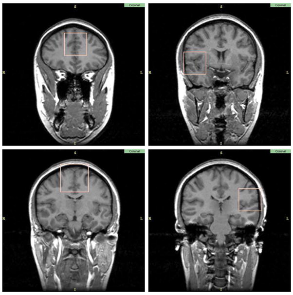
Sub-regions of the brain selected for manual labeling.

For each of the twenty scans, three experts manually labeled the four sub-regions into BG, GM, WM and CSF.

3.5 Statistical Analyses

3.5.1 Evaluation with no manual segmentation reference

Let X_il = {x, I_i(x) = l} be the set of voxels labeled l by rater i. Let ASRE (Automatic Segmentation Reference Estimate) be the estimated reference computed by STAPLE from all eleven multi-categorical label maps, with ASRE_l the set of voxels labeled l in ASRE. For each subject, for each label, different types of analysis were done. First, Williams’ index was computed for each label using the eleven X_il as input and JC as the agreement measure. Second, for each rater, the JC between X_il and the reference estimate for that label ASRE_l were computed. The mean and standard deviation of the Williams’ index and JC score against ASRE_l over all subjects are shown in figure 4. The probability that rater j labels a voxel with s′ when the ASRE label is s (the confusion matrices θ_j(s′, s) obtained by STAPLE) are represented in figure 5. In the figure each table represents the average θ_j(s′, s) for a particular algorithm over all cases. The color coding used in the figure gives another visual cue for assessing the quality of the segmentation. A good algorithm will display bright coloring in the diagonal and dark coloring everywhere else. Gray regions generally indicate poor performance. Finally, MDS plots were generated based on the average of forty interdistance matrices. Each matrix had 12×12 values corresponding to one minus the similarity measure between each one of the eleven segmentation as well as ASRE. The plots are shown in figures 6.

Fig. 4.

Mean/std plots: Top, JC score against STAPLE’s ASRE; Bottom, Williams’ Index. Red: WM score, Green: GM score, Blue: CSF score.

Fig. 5.

Confusion matrices provided by STAPLE. The grayscale is a visual cue to better evaluate the quality of the segmentation, bright coloring in the diagonal and dark coloring off-diagonal indicate good performance. For each matrix, the rows represent the labels of the ASRE and the columns the labels of the observed segmentation. Note the matrices are not symmetric.

3.5.2 Evaluation with a manual segmentation reference

Let MSRE (Manual Segmentation Reference Estimate) be the estimated reference computed by STAPLE from all three manual segmentations of the subregions, with MSRE_l the set of voxels labeled l in MSRE. First, for each of the twenty subjects, for each label, Williams’ index was computed using JC as a metric and the eleven X_il as input, but only on the sub-regions used for the manual tracing. Second, for each subject, ASRE_l was recomputed but only based on the sub-regions used for the manual tracing. JC was then measured between the sub-regions of X_il and the new ASRE_l. Third, for each rater, JC was measured between X_il and MSRE_l (which is only defined on the subregions used for the manual tracing). The mean and standard deviation of the Williams’ index and JC score against ASRE and MSRE over all subjects are shown in figure 7. MDS plots were also generated based on the average JC table over all twenty subjects. Each matrix had 16 × 16 values corresponding to one minus the JC on the sub-regions between the eleven segmentations, the three manual segmentations, MSRE and the new ASRE. The plots are shown in figure 8.

Fig. 7.

Top, Williams’ Index; Middle, JC score against the new ASRE (only based on the sub-regions); Bottom, score against MSRE. The similarities were only computed over four small sub regions of the brain. Red: WM score, Green: GM score, Blue: CSF score.

Fig. 8.

The JC matrices are represented by 2D maps through MDS (left). Residual plots for the mapping are given to assess the quality of the mapping (right). The similarities were computed over four small sub regions of the brain.

4 Results

4.1 Evaluation with no manual segmentation reference

Figure 4 presents the mean/standard deviation plots of JC. Our first observation is that for GM and WM, Williams’ index and STAPLE give a very similar ordering, whereas for CSF they are quite different. This might be due to the difficulty of segmenting CSF, which leads to higher variability and lower accuracy of the output, and consequently less reliable agreement measurements.

Concerning the ranking of techniques, a few observations can be made. First, we have the surprising result that single channel segmentation performs usually better than dual channel. This is especially true for FSL, where we suspect the algorithm was not tuned properly for multiple inputs. Another reason might be the low resolution of the T2 image, which could have the indirect effect of blurring the input thus leading to a less accurate segmentation. According to the STAPLE output, FSL1 scores best for CSF, GM and WM. According to Williams’ index FSL1 scores best for CSF; KNN1, FSL1 and SPM1 are first for GM; KNN1, FSL1 and WAT2 are best for WM. Overall, FSL1 is the best classifier according to both ASRE and William’s index.

The next set of plots we analyze are the θ_j confusion matrices provided by STAPLE shown in figure 5. Having the full confusion matrices is interesting as it allows us to detect not only which tissue is misclassified but also which wrong tissue it is likely to be labeled. Overall, all algorithms perform quite well. The most common mistake is the classification of CSF into either BG or GM.FSL2 also often classifies voxels WM that, according to ASRE, truly are GM. It is important to note these matrices are not symmetric. The probability of an algorithm labeling a voxel BG when ASRE is CSF (quite likely) is different than the probability of labeling CSF when ASRE is BG (highly unlikely).

We now turn to the analysis of the MDS configurations presented in figures 6. These plots are based on the JC inter-dissimilarity matrix, which is represented as Euclidean distances on a 2D layout. STAPLE estimated reference is represented in red with label ASRE. We first note that the residual plots between true distances and mapped distances indicate that the MDS are all quite good. These plots are interesting because they not only show how close classifiers are to the reference but also how close they are to each other. For CSF, FSL1 is clearly closest to ASRE and there seems to be a cluster FSL1, FSL2, MNI1, KNN1 and KNN2, although FSL2 is highly variable. For GM, we see a tight cluster around ASRE formed by WAT2, SPM2, SPM1, FSL1 and KNN1 corresponding to the best techniques according to figure 4. For WM, there is a number of techniques which perform well, FSL1 being best, followed closely by WAT2, KNN1 and EMA2 then SPM1, SPM2 and MNI1. Overall, one can see the poor performance and high variability of FSL2. EMS2 is also often in the position of an outlier although it usually has very low variability. It is also interesting to observe that ASRE is placed near the center in the GM and WM plots. It illustrates well the notion of a reference segmentation as a weighted average of multiple rater classifications. Finally, there is no clear cluster of methods that are very similar to each other and except for outliers it would be difficult to extract 2 or 3 different categories of classifiers based on the MDS plots presented here.

Another important aspect of classifier performance, is its robustness. Both Mean/Std plots and MDS plots give a us a good insight of how variable classifiers are. It is important to note that some classifiers may have a good mean score but not a great standard deviation (e.g. EMA2). In this experiment, FSL1, SPM2 and SPM1 have very low variability across all labels and measurements which are very desirable features in neuroimaging studies.

In summary, even though no manual segmentation was used as a reference, we were able to gather interesting facts about the classifiers and the evaluation methodologies. First, it seems that computing a reference segmentation using STAPLE is not necessary to evaluate segmentation techniques and that the simpler Williams’ index provides very similar results. The use of MDS plots allows for a nice overview of the inter-similarity of all the classifiers and how close they are to a reference segmentation. We also observed the somewhat surprising result that two input channels can be worse than one, especially if the algorithm is not properly tuned for it, as we suspect for FSL2. Finally, even though there are winners and losers in our performance evaluation, we find that most classifiers are close to each other and that no clear clustering can be done between them. We now turn to the validation of our evaluation techniques by introducing manually segmented sub-regions of the brain as the gold standard.

4.2 Evaluation with a manual segmentation reference

In the next few figures, we present a validation of our evaluation techniques, as described in section 3.5.2. Individual segmentations of subsets of twenty brains are compared against each other, STAPLE’s ASRE, as well as MSRE, the manual segmentation reference estimate based on manual tracings from three expert human raters.

In the mean/std plots (figure 7), we have the following ordering. For CSF, FSL1 is ranked first according to William’s Index, STAPLE ASRE, and STAPLE MSRE. For GM, Williams’ index rates SPM1 first, and WAT2 second. According to STAPLE ASRE, FSL1 and SPM1 are first with KNN1, EMA2 and WAT2 rated second. For STAPLE MSRE, SPM1 is first and FSL1 is second. For WM, EMA2 is ranked first by Williams’ index, WAT2 is second. EMA2 is first, FSL1 and WAT2 are second, when compared to STAPLE ASRE. STAPLE MSRE rates EMA2 first with FSL1 and SPM1 second. Table 3 shows the ranking assigned to each classifier by the different evaluation methods. Overall the ordering is quite similar and the same five or six classifiers share the top three spots for all measures. We note also a slightly different ordering than in section 4.1, due to the smaller number of subjects and dramatically smaller number of voxels tested (the entire cerebellum and basal ganglia have been ignored). In the MDS plots (figure 8), we have displayed all eleven segmentations, the three manual raters, and two STAPLE reference estimates: one based only on the automatic classifiers (ASRE) and one based only on the manual raters (MSRE). The residual plots between true distances and the MDS mapping distances are still quite good, although the 2D mapping seem to underestimate shorter distances and overestimate large ones. The interesting result here is that it is possible to visually separate the three manual segmentations from the eleven automatic ones. One can almost see two clusters, (i) manual raters and (ii) automatic classifiers. Even more interesting is the fact that ASRE is relatively far from MSRE, suggesting that a manual segmentation is indeed necessary for accurately assessing the performance of segmentation results. We further explore this fact by looking at JC against MSRE for the top performer in each class, ASRE and the manual segmentations. Our results are presented in figure 9. For each tissue class, ASRE does not perform as well as the best automatic classifier and all automatic classifiers significantly underperform compared to the manual raters. One should also note the relatively higher variability of the manual raters’ scores compared to more consistent automatic techniques.

Table 3.

Rank ordering of the classifiers by the different evaluation techniques on the subregion data in 20 cases. The number in each entry corresponds to the ranking of the technique according to the measurement.

	kNN2	kNN1	MNI2	MNI1	FSL2	FSL1	SPM2	SPM1	EMS2	EMA2	WAT2
Williams JC WM	9	5	11	7	10	3	6	4	8	1	2
JC vs. ASRE WM	10	5	9	4	11	3	7	6	8	1	2
JC vs. MSRE WM	10	5	9	4	11	3	7	2	8	1	6
Williams JC GM	8	4	9	7	11	3	5	1	10	6	2
JC vs. ASRE GM	8	3	9	6	11	1	7	2	10	5	4
JC vs. MSRE GM	9	3	10	4	11	2	6	1	8	5	7
Williams JC CSF	9	4	8	6	10	1	3	2	11	7	5
JC vs. ASRE CSF	6	4	10	2	5	1	7	3	11	9	8
JC vs. MSRE CSF	8	5	10	3	9	2	4	1	11	6	7

Fig. 9.

JC score against STAPLE MSRE: Red, WM; Green, GM; Blue, CSF. The top in each class is represented (FSL1 for CSF, SPM1 for GM and EMA2 for WM).

With respect to variability, FSL1 and MNI1 are very good performers. One should also note the relatively high variability of the manual segmenters, reinforcing the idea that building ground truths based on a single expert rater may not be the best approach.

5 Discussion

5.1 Common Agreement and Bias

The main hypothesis underlying the common agreement principle is the notion that each classifier makes decisions independently from the others. In fact, it is more complex as this independence is conditioned by the underlying truth and the performance parameters of each classifier. This notion is central to both Williams’ Index and STAPLE. As the truth and performance are not known a priori, one cannot test for independence and generally needs to assume classifiers make highly uncorrelated mistakes. Given our seven segmentation methods, one could wonder whether our results are not biased towards a subgroup of them. Our main concerns are the following. First, FSL, EMS, EMA, SPM are all EM algorithms and it is possible they have similar behaviors and bias the common agreement. Second, as pointed out in section 3.2, many of the algorithms rely on training data and/or a spatial prior atlas. It is also likely that techniques with the same atlas will have similar outputs.

Luckily, in our experiments, we have designed a reference standard based on manual segmentation and we can further investigate this notion of independent decisions. In order to test for the potential biases, we performed the following experiment: for each segmentation output and each label, an image of all wrongfully labeled voxels was created as a binary volume in which all False Positive and False Negative voxels have been assigned the value 1. This process was done for all classifiers over all cases where manual segmentations were traced. MSRE was used as the ground truth segmentation to decide which voxels were misclassified. All resulting error maps were then compared to each other using JC. In essence, we are trying to evaluate the amount of overlap of the errors made by each classifier. A plot where all classifiers are at equal (preferably large) distance from each other would be ideal. Of note, the expected distance (1-JC) between two randomly generated images is 2/3. Thus an observed distance over 0.5 would be very encouraging. Our observation is that the overall distance between each segmentation method is fairly homogeneous. The average inter-classifier (1-JC) value is 0.65, with 0.07 standard deviation; the minimum distance is 0.44.

MDS plots were created to inspect the data and detect possible clusters (figure 10). The residual plot show significant disagreement between the (1-JC) matrices and the 2D distances. It could be due to the fact that all classifiers are equally distant from each other, making the mapping extremely difficult. Unfortunately, one cannot make this conclusion purely based on the plots, so one should be careful not to draw strong statements from these plots. For GM and WM, the data cannot be easily assigned to clusters, but some similarity trends are observable. SPM1 and SPM2 are always quite close to each other, KNN1, KNN2 and WAT2 also tend to be quite close, especially when segmenting GM. Note that the 2D MDS plot may show different distances as the mapping from high dimensional space to 2D distorts the distances. The techniques are thus not entirely uncorrelated, but it appears they make reasonably independent decisions, or more accurately, independent misclassifications. We are thus confident that the common agreement is not strongly favoring a specific subset of techniques. For CSF however, one can see that there is an observable separation between two channels and one channel classifiers. Indeed it is not too surprising as CSF is almost not visible in T1w images. This may result in a bias when comparing one to two channel results. In addition, manual segmentations were only performed on T1 images and the MSRE is thus biased. Further experiments would be needed in order to thoroughly address the effect of this bias on the results for CSF when comparing one to two channel algorithms.

Fig. 10.

Testing Independence: MDS maps and their residual plots of the JC matrices of the classifiers’ error maps (containing both False Positive and False Negative).

5.2 Scalability

One important aspect of the evaluation framework presented here is whether the notion of common agreement scales well. Assume that we had a complete evaluation, without a ground truth, of twenty classifiers, it is possible that one could choose ten classifiers out of the twenty, rerun the evaluation on only those and get completely different rankings than when using all twenty. In order to test for this eventuality, one could create all combinations of subsets of size 3 to n−1 classifiers, and compare the results with the n classifiers evaluation. Unfortunately, the combinatorial nature of this process would imply a unreasonably large number of experiments to perform (1980 for a total of 11 classifiers). We thus computed the JC against STAPLE’s standard reference estimate on the full data set without ground truth but only using 8 classifiers, 6 classifiers, and 4 classifiers. We present the results in figure 11 as mean/std plots of JC scores against each newly created automatic segmentation reference estimate. Our observation is that although the performance measurement varies as the common agreement is built from a subset of the classifiers, the ranking scales quite well, even when only 4 classifiers are used.

Fig. 11.

Testing Scalability: In this experiment, different subsets of the classifiers were compared (top left, all 11 classifiers; top right, 8 classifiers; bottom left, 6; bottom right, 4). Although the exact performance measure differs from experiment to experiment, the respective rankings of the classifier is relatively well preserved. Red, WM; Green, GM; Blue, CSF.

5.3 Using a Standard Ground Truth

We have claimed that it is essential to test the algorithms on our data set in order to get a sensible assessment of performance for our specific segmentation problem. Nevertheless, in this section we check if one can get similar results using a readily available ground truth. To our knowledge no publicly available data repository exists with manually delineated WM, GM and CSF of the entire brain and two inputs similar to our data set (T1w and T2w). There are data sets that have a T1w image and nice segmentations of the gray matter such as the Internet Brain Segmentation Repository (http://www.cma.mgh.harvard.edu/ibsr/data.html), but they rarely have CSF segmentations or multiple input images (e.g. T1w, T2w and PD). We thus turned to the Montreal Neurological Institute (MNI) normal brain phantom (http://www.bic.mni.mcgill.ca/brainweb/) and downloaded the following sequences: a T1 weighted image and a T2 weighted both with voxel size of 1mm³, 3% noise and 20% intensity inhomogeneities (Collins et al., 1998). We then ran all segmentation algorithms on this single case and compared the outputs to the ground truth provided by the MNI. The results are presented in figure 12. As we expected, the results are quite different from the ones observed on our own data set. The MNI algorithms tend to perform best, as they may have been trained on this particular ground truth, which would bias the performance evaluation. One should note however that it is difficult to make a fair comparison as this is only one case and that variability and robustness cannot be assessed in this context.

Fig. 12.

Evaluating performance on a synthetic generated brain from the Montreal Neurological Institute. Red, WM; Green, GM; Blue, CSF.

5.4 Testing Performance Variability in the Evaluation Measurements

An important question which has to be answer is whether the variability in the evaluation measurements analyzed along the paper comes from the variability within algorithms due to the finite nature of the data (40 cases were used) or whether it can truly be attributed to the variability among algorithms, the latter allowing the ranking among algorithms to make sense. Several approaches can be used to answer this question. One possible solution is to select pairs of algorithms and to run a student t test in order to know whether the evaluation measurements for two algorithms are significantly different from each other. However, this means 55 tests for each label and for each measurement which is far too many tests to perform. Another simple solution to have some insight into this problem is to run a one-way ANOVA F test to reject the hypothesis that all 11 classifiers perform similarly for a given measurement.

In table 4 the obtained results are shown for labels WM, GM and CSF using the JC as the similarity measure with respect to ASRE and the Williams’ index using JC as well. The obtained p-values are always lower than 0.0001 which means that all the tests were passed and that the variability among the evaluation measurements are truly due to differences among the raters (algorithms). Finally, a last set of tests using the MSRE were also performed. In this case, we use only the sub-regions for which the manual segmentations were performed for 20 out of the 40 subjects. The tests were run for the same measurements as before: JC with respect to ASRE, the Williams’ index using JC and, in addition, JC with respect to MSRE, as for the sub-regions MSRE is available. Similar p-values are achieved as shown in table 5: the analyzed measurements clearly indicate that the algorithms behave significantly different.

Table 4.

Results for the one-way ANOVA F test showing that the evaluation measurements among the algorithms are truly different. The whole 40 data sets are used.

One-way ANOVA	k − 1 df	n − k df	F	p
JC vs. ASRE WM	10	30	27.25	<0.0001
JC vs. ASRE GM	10	30	23.85	<0.0001
JC vs. ASRE CSF	10	30	136.02	<0.0001
Williams JC WM	10	30	23.55	<0.0001
Williams JC GM	10	30	22.76	<0.0001
Williams JC CSF	10	30	51.13	<0.0001

Table 5.

Results for the one-way ANOVA F test showing that the evaluation measurements among the algorithms are truly different. The sub-regions for which manual segmentations are available were used (20 subjects).

One-way ANOVA	k − 1 df	n − k df	F	p
JC vs. MSRE WM	10	10	9.56	<0.0001
JC vs. MSRE GM	10	10	9.72	<0.0001
JC vs. MSRE CSF	10	10	14.14	<0.0001
JC vs. ASRE WM	10	10	8.00	<0.0001
JC vs. ASRE GM	10	10	8.22	<0.0001
JC vs. ASRE CSF	10	10	30.88	<0.0001
Williams JC WM	10	10	9.02	<0.0001
Williams JC GM	10	10	6.45	<0.0001
Williams JC CSF	10	10	16.04	<0.0001

6 Conclusion

In this paper, we investigated evaluating automatic segmentation without having a ground truth. Common agreement was used as the foundation of our comparison study. We chose the Jaccard Coefficient as a metric to measure agreement between two segmentations. We then used three different methods to evaluate and visualize the notion of common agreement. Of these three methods, the Williams’ Index provided us with a simple and efficient way of measuring whether a particular classifier agreed with all other classifiers as much as they agreed with each other. STAPLE provided a more comprehensive tool by simultaneously computing the performance of each algorithm and creating a reference segmentation based on their outputs. Finally, MDS allowed us to visually assess the similarity between all the different segmentations.

Using these three techniques, we ran a set of experiments to evaluate 11 different classifiers over 40 data sets. First, we found that Williams’ Index and STAPLE give very similar results, so that for a quick study we would recommend the use of Williams’ Index as it is much faster to compute. We also found the MDS plots very informative to quickly inspect the data and detect possible clusters. With regards to algorithm performance, our findings suggest that most classifiers tested perform quite well, except for FSL2. We also found that FSL1 tends to get better performance overall.

We also validated our evaluation techniques by creating a reference standard based on expert raters’ manual segmentations. Unfortunately, due the size of the images and the number of cases, human experts traced only four small sub-regions of the brain in twenty cases. A reference estimate was then created for these four regions by combining all experts’ segmentations using STAPLE. The evaluation procedures were repeated but only using the subset of data for which we had this partial ground truth. We found that the ranking of the segmentation techniques was similar whether they were compared to common agreement or ground truth. However, our results also showed that the expert raters did have a common notion of truth that was not detected by the automatic classifiers. The MDS plots were especially interesting as they showed two distinct clusters of classifiers: the human raters on one side and the automatic segmentation algorithms on the other side, suggesting that our experts shared some prior knowledge not properly modeled by automated classifiers.

Other considerations such as possible bias towards a subgroup of the different classifiers, scalability and a discussion on using a unrepresentative ground truth have been presented. We found that our selection of classifiers was well balanced, that our technique scales well, even when only a few classifiers are used to compute agreement, and that using a ground truth that does not accurately represent our data set can give very different performance results.

Overall, we feel confident that a number of interesting and important observations can be made from an evaluation pipeline based on common agreement alone. That is, outliers can be easily detected, strongly consistent or highly variable techniques can be readily discriminated, the overall similarity between different techniques can be assessed, and a reasonable ranking of techniques can be established. However, we also note that common agreement has to be used with special care. For instance, if one algorithm clearly outperforms the others, it will be considered an outlier which is clearly undesirable. This is unlikely to happen in practice, especially for brain tissue segmentation, as the field is mature and techniques tend to perform similarly. Nevertheless, if one needs refined measurements of segmentation accuracy, a carefully designed ground truth is desirable. We conclude that although not perfect, using evaluation techniques purely based on common agreement is certainly meaningful.

References

- Ashburner J, Friston K. Spatial normalization using basis functions. In: Frackowiak RSJ, Friston KJ, Frith C, Dolan R, Friston KJ, Price CJ, Zeki S, Ashburner J, Penny W, editors. Human Brain Function. 2. Academic Press; 2003. [Google Scholar]
- Borg I, Groenen P. Modern Multidimensional Scaling: Theory and Applications. Springer-Verlag; New York: 1997. [Google Scholar]
- Chalana V, Kim Y. A methodology for evaluation of boundary detection algorithms on medical images. IEEE Transactions on Medical Imaging. 1997;16 (5):642–652. doi: 10.1109/42.640755. [DOI] [PubMed] [Google Scholar]
- Collins DL, Zijdenbos AP, Kollokian V, Sled JG, abani NJ, Holmes CJ, Evans AC. Design and construction of a realistic digital brain phantom. IEEE Transactions on Medical Imaging. 1998;17 (3):463–468. doi: 10.1109/42.712135. [DOI] [PubMed] [Google Scholar]
- Cox TF, Cox MAA. Multidimensional Scaling. 2. Chapman & Hall/CRC; 2000. [Google Scholar]
- Gerig G, Jomier M, Chakos M. Valmet: A new validation tool for assessing and improving 3D object segmentation. International Conference on Medical Image Computing and Computer-Assisted Intervention; 2001. pp. 516–523. [Google Scholar]
- Grau V, Mewes AUJ, Alcañiz M, Kikinis R, Warfield SK. Improved watershed transform for medical image segmentation using prior information. IEEE Transactions on Medical Imaging. 2004;23 (4):447–458. doi: 10.1109/TMI.2004.824224. [DOI] [PubMed] [Google Scholar]
- Hripcsak G, Heitjan DF. Measuring agreement in medical informatics reliability studies. Journal of Biomedical Informatics. 2002;35:99–100. doi: 10.1016/s1532-0464(02)00500-2. [DOI] [PubMed] [Google Scholar]
- Jaccard P. Étude comparative de la distribuition florale dans une portion des alpes et de jura. Bulletin de la Societé Voudoise des Sciences Naturelles. 1901;37:547–579. [Google Scholar]
- Klingensmith JD, Shekhar R, Vince DG. Evalutation of three-dimensional segmentation algorithms for the identification of luminal and medial-adventitial borders in intravascular ultrasound images. IEEE Transactions on Medical Imaging. 2000;19 (10):996–1011. doi: 10.1109/42.887615. [DOI] [PubMed] [Google Scholar]
- Krissian K. Flux-based anisotropic diffusion applied to enhancement of 3-D angiograms. IEEE Transactions on Medical Imaging. 2002;21 (11):1440–1442. doi: 10.1109/TMI.2002.806403. [DOI] [PubMed] [Google Scholar]
- Martin-Fernandez M, Bouix S, Ungar L, McCarley RW, Shenton ME. Two methods for validating brain tissue classifiers. International Conference on Medical Image Computing and Computer-Assisted Intervention; 2005. pp. 515–522. [DOI] [PMC free article] [PubMed] [Google Scholar]
- Pohl KM, Bouix S, Kikinis R, Grimson WEL. Anatomical guided segmentation with non-stationary tissue class distributions in an expectation-maximization framework. IEEE International Symposium on Biomedical Imaging; Arlington, VA. Apr, 2004. pp. 81–84. [DOI] [PMC free article] [PubMed] [Google Scholar]
- Rex DE, Shattuck DW, Woods RP, Narr KL, Luders E, Rehm K, Stolzner SE, Rottenberg DA, Toga AW. A meta-algorithm for brain extraction in MRI. NeuroImage. 2004;23:625–627. doi: 10.1016/j.neuroimage.2004.06.019. [DOI] [PubMed] [Google Scholar]
- Rohlfing T, Russako3 DB, Maurer CR. Expectation maximization strategies for multi-atlas multi-label segmentation. Information Processing in Medical Imaging. 2003a:210–221. doi: 10.1007/978-3-540-45087-0_18. [DOI] [PubMed] [Google Scholar]
- Rohlfing T, Russako3 DB, Maurer CR. Extraction and application of expert priors to combine multiple segmentations of human brain tissue. International Conference on Medical Image Computing and Computer-Assisted Intervention; 2003b. pp. 578–585. [Google Scholar]
- Sammon JW. A nonlinear mapping for data structures analysis. IEEE Transactions on Computers C-18. 1969;(5):401–409. [Google Scholar]
- Schwartz EL, Shaw A, Wolfson E. A numerical solution to the generalized mapmaker’s problem: Flattening nonconvex polyhedral surfaces. IEEE Transactions on Pattern Analysis and Machine Intelligence. 1989;11 (9):1005–1008. [Google Scholar]
- Sled JG, Zijdenbos AP, Evans AC. A non-parametric method for automatic correction of intensity non-uniformity in MRI data. IEEE Transactions on Medical Imaging. 1998;17 (1):87–97. doi: 10.1109/42.668698. [DOI] [PubMed] [Google Scholar]
- Smith S. Fast robust automated brain extraction. Human Brain Mapping. 2002;17 (3):143–155. doi: 10.1002/hbm.10062. [DOI] [PMC free article] [PubMed] [Google Scholar]
- Warfield S. Fast kNN classification for multichannel image data. Pattern Recognition Letters. 1996;17 (7):713–721. [Google Scholar]
- Warfield SK, Zou KH, Kaus MR, Wells WM. Simultaneous validation of image segmentation and assessment of expert quality. International Symposium on Biomedical Imaging; 2002a. pp. 1–4. [Google Scholar]
- Warfield SK, Zou KH, Wells WM. Validation of image segmentation and expert quality with an expectation-maximization algorithm. International Conference on Medical Image Computing and Computer-Assisted Intervention; 2002b. pp. 298–306. [Google Scholar]
- Warfield SK, Zou KH, Wells WM. Simultaneous truth and performance level estimation (STAPLE): An algorithm for the validation of image segmentation. IEEE Transactions on Medical Imaging. 2004;23:903–921. doi: 10.1109/TMI.2004.828354. [DOI] [PMC free article] [PubMed] [Google Scholar]
- Wells WM, Kikinis R, Grimson WEL, Jolesz F. Adaptive segmentation of MRI data. IEEE Transactions on Medical Imaging. 1996a;15:429–442. doi: 10.1109/42.511747. [DOI] [PubMed] [Google Scholar]
- Wells WM, Viola P, Atsumi H, Nakajima S, Kikinis R. Multimodal volume registration by maximization of mutual information. Medical Image Analysis. 1996b;1:35–52. doi: 10.1016/s1361-8415(01)80004-9. [DOI] [PubMed] [Google Scholar]
- Williams GW. Comparing the joint agreement of several raters with another rater. Biometrics. 1976;32:619–627. [PubMed] [Google Scholar]
- Xu L, Krzyzak A, Suen CY. Methods of combining multiple classifiers and their applications to handwriting recognition. IEEE Transactions on Systems, Man and Cybernetics. 1992;22 (3):418–435. [Google Scholar]
- Yoo TS, Ackerman MJ, Vannier M. Toward a common validation methodology for segmentation and registration algorithms. International Conference on Medical Image Computing and Computer-Assisted Intervention; 2000. pp. 422–431. [Google Scholar]
- Zhang Y, Brady M, Smith S. Segmentation of brain MR images through a hidden markov random field model and the expectation maximization algorithm. IEEE Transactions on Medical Imaging. 2001;20 (1):45–57. doi: 10.1109/42.906424. [DOI] [PubMed] [Google Scholar]
- Zijdenbos AP, Dawant BM, Margolin RA, Palmer AC. Morphometric analysis of white matter lesions in MR images: Method and validation. IEEE Transactions on Medical Imaging. 1994;13 (4):716–724. doi: 10.1109/42.363096. [DOI] [PubMed] [Google Scholar]
- Zijdenbos AP, Forghani R, Evans AC. Automatic “pipeline” analysis of 3-D MRI data for clinical trials: application to multiple sclerosis. IEEE Transactions on Medical Imaging. 2002;21 (10):1280–1291. doi: 10.1109/TMI.2002.806283. [DOI] [PubMed] [Google Scholar]