Estimating the posterior probability that genome-wide association findings are true or false

Abstract

Motivation: A limitation of current methods used to declare significance in genome-wide association studies (GWAS) is that they do not provide clear information about the probability that GWAS findings are true of false. This lack of information increases the chance of false discoveries and may result in real effects being missed.

Results: We propose a method to estimate the posterior probability that a marker has (no) effect given its test statistic value, also called the local false discovery rate (FDR), in the GWAS. A critical step involves the estimation the parameters of the distribution of the true alternative tests. For this, we derived and implemented the real maximum likelihood function, which turned out to provide us with significantly more accurate estimates than the widely used mixture model likelihood. Actual GWAS data are used to illustrate properties of the posterior probability estimates empirically. In addition to evaluating individual markers, a variety of applications are conceivable. For instance, posterior probability estimates can be used to control the FDR more precisely than Benjamini–Hochberg procedure.

Availability: The codes are freely downloadable from the web site http://www.people.vcu.edu/∼jbukszar.

Contact: jbukszar@vcu.edu

Supplementary information: Supplementary data are available at Bioinformatics online.

1 INTRODUCTION

In genome-wide association studies (GWAS) it is important to assess as accurately as possible whether findings are likely to be true or false. Erroneous conclusions would result in either false discoveries or false non-discoveries. Avoiding false discoveries is important to prevent the waste of time and resources spent on GWAS leads that will eventually prove irrelevant for the outcome of interest. False non-discoveries are undesirable because of the missed opportunity to detect genetic variants that do affect disease susceptibility and eventually could, for example, improve the management and treatment of the disease.

Although only a comprehensive set of follow up studies (e.g. replication, functional and animal studies) can establish decisively whether or not individual marker disease associations are real findings, GWAS are potentially very informative. A problem is that current statistical methods are limited in their ability to use this information to provide the critical initial assessment about the probability that GWAS findings are true or false. For example, setting a genome-wide significance threshold that accounts for the number of tests that are performed does not provide any assurance that the associations found to be significant are genuine (Zaykin and Zhivotovsky, 2005). This is because the probability that the significant marker is real does not only depend on the chance of being a false discovery, but also on the statistical power to detect true associations. More precisely, if the statistical power is higher then significant markers are more likely to be true. This is the reason why significant findings obtained from a large GWAS study, or meta analysis of several large studies, are more likely to be true. The problem is that this information is not available from standard methods testing for genome-wide significance. Conversely, it may also be the case that markers not reaching genome-wide significance have real effects. If statistical power is modest, markers with real effects may not even be among the top findings. In these scenarios, following up just the top findings is problematic as the markers with real effects would be excluded from further consideration. Clearly, regardless of whether or not they reach genome-wide significance, knowledge about the probability that individual markers have real effects would be of considerable value to better evaluate GWAS findings and inform follow up studies.

For assessing the probability that GWAS findings are true or false, false discovery rate (FDR)-based methods (Benjamini and Hochberg, 1995, 2000; Storey and Tibshirani, 2003; Storey et al., 2004; Storey, 2002, 2003) offer some advantages over the commonly used multiple testing methods that correct for multiple testing to control false discoveries (e.g. Bonferroni correction). For example, controlling the FDR at the 0.1 level would ensure that on average 10% of all significant findings can be expected to be false or 90% of all significant findings are expected to be true. At least for the group of significant markers as a whole, FDR methods do provide insight into the expected proportion of false/true discoveries. However, the FDR essentially averages the probabilities that individual markers are false discoveries across the whole group of significant markers. Therefore, it does not provide marker-specific information (Finner and Roters, 2001; Glonek and Soloman, 2003). One consequence of this averaging is that a marker with very high probability of being a false discovery may still be significant with a low-FDR level because it is tested simultaneously with unrelated markers that do have very low probabilities of being a false positive. Glonek et al. (Glonek and Soloman, 2003), for example, give a numerical example where a marker has a 90% chance of being a false discovery, but is still significant at an FDR level of 0.1.

So-called q-values are FDRs calculated by using the p-value of the markers as the threshold for declaring significance (Black, 2004). At first sight, q-values do seem to provide some marker-specific evidence of being a false discovery. This is because each marker has a specific q-value. However, q-values are also subject to limitations arising from averaging probabilities of being a false discovery across the entire region, and can therefore not be interpreted as the probability of that marker being a false discovery. For example, the smallest q-value estimates the average probability of all hypothetical markers in the entire rejection region, which is the region where test statistic values are larger than the one of the marker with the smallest q-value. Having the smallest test statistic of all hypothetical markers in the entire rejection region, the marker with the smallest q-value itself has the highest probability of being a false discovery in the whole rejection region. Thus, the probability of the most significant marker being a false discovery will always be higher than the q-value, rendering a marker-specific interpretation problematic.

To more accurately assess whether GWAS markers have true effects and to improve marker selection for follow up studies under a wide variety of possible strategies, we need to estimate the posterior probability that a particular marker has a certain effect given its test statistic value in a GWAS. In contrast to conventional multiple testing methods that determine significance or non-significance without having a clear sense of significant markers having a real effect and non-significant markers not having real effects, posterior probabilities provide a more subtle picture and allow more informed decisions about which markers to follow up. Furthermore, because posterior probabilities condition on the observed test statistic value rather than on a whole rejection region, they do not suffer from the above discussed ‘averaging’ effect of the FDR and q-values.

The specific posterior probability that the effect is zero is also known as the local FDR (ℓFDR) (Efron et al., 2001). The ℓFDR is a fairly commonly applied tool in expression array research, where they are usually estimated using non-parametric techniques (Aubert et al., 2004; Dalmasso et al., 2005, 2007; Liao et al., 2004; Ploner et al., 2006; Scheid and Spang, 2004). However, these non-parametric ℓFDR estimates tend to have large standard errors and be imprecise (Aubert et al., 2004; Dalmasso et al., 2007; Liao et al., 2004). The reason is that we need to estimate the mixture of the two densities, i.e. the null (f₀) and alternative (f_ε) densities, which is typically done by creating discrete bins across the possible values of the test statistic in the non-parametric case. To remedy the precision problem, some parametric ℓFDR estimators have been designed for analyzing expression array data (Allison et al., 2002; Pounds and Morris, 2003). However, these parametric approaches use an approximation of the test statistic distribution under the alternative that, to the best of our knowledge, is never used in the context of GWAS (e.g. a special case of the beta distribution). More typically, one would use Pearson's statistic or (logistic) regression analyses in GWAS, where the test statistic distribution is approximated by (non-central) chi-square, F or normal distributions. Furthermore, in GWAS, we typically have a large number (>=500 000) of markers and only few of them have real effects.

In this article, we develop a precise method for estimating the ℓFDR. Our estimator takes advantage of the facts that in GWAS, we often have good parametric approximations of the density functions for most tests performed and that the number of markers with effects is likely to be small. Furthermore, a first and critical step of our method is to estimate the (non-centrality) parameters of the densities under the alternative. Instead of the widely used mixture model likelihood function that is a rough approximation, we used the real maximum likelihood function to avoid a loss of precision. Our approach is tested through simulations and illustrated with empirical GWAS data.

2 METHODS

2.1 The concept of effect size and detectability

First, we need to clarify what we mean by effect. We mean a marker has a real effect in a statistical sense that is we say that a marker has real effect if the probability of the occurrence of the alleles at the marker locus is different for affected and unaffected individuals. Note that this is not exactly the same as ‘causal’ in a biological sense. That is not only the causal markers, but also the markers in strong LD with a causal marker may/will have real effects. For instance, a marker that tags a true association due to close proximity to a causal marker will have a real effect. Further examples of statistical effects may be due to technical errors or population stratification. Note that no statistical method can distinguish between the different type of effects.

In what follows we will deal with test statistics whose distribution or approximating distribution under the alternative depends on a single parameter only, which we call effect size. Note that the alternative distribution also depends on the sample size, which is, however, a known parameter, therefore we do not need to estimate it. For instance, for case–control allele-based studies, Pearson's statistic under the alternative hypothesis is frequently approximated by the non-central distribution with non-centrality parameter nθ², where n is the sample size and θ is the effect size. In practice, we actually estimate this non-centrality parameter, from which the effect size can be readily calculated. Therefore, we shall refer to the square root of non-centrality parameter under the alternative hypothesis as detectability. The rationale of taking the square root is that the detectability is linearly proportional to the effect size (twice as big effect size has twice as big detectability, in the same study). In general, the detectability is defined as the product of the root of the sample size and the (suitably chosen) single parameter of the alternative distribution.

2.2 The underlying problem

Suppose m hypothesis tests are performed with statistics T₁,…, T_m. Exactly m₀ of the m statistics follow the null distribution and the rest of them m₁ = m − m₀ follow the alternative distribution whose density function is known, but depends on only a single unknown parameter, called effect size that may vary across the alternative hypotheses.

2.3 Parametric estimator of the ℓFDR

2.3.1 Estimating individual detectabilities

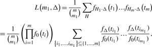
For estimating the posterior probability that a marker has zero detectability, we will utilize our individual detectability estimates (Supplementary Material), which we outline first. We initially estimate the average detectability Δ. To estimate Δ, for now we make the crude assumption that all individual detectabilities are identical, and use the ML method to estimate it. The likelihood function on the test statistic values t₁,…, t_m, assuming equal detectabilities Δ for all true alternative hypotheses, can be obtained in the following way. Let H_i=0 when null hypothesis i is true, and H_i=1 otherwise. Note that vector H=(H₁,…, H_m) has m₀=0 and m₁=1 components. We assume that H=(H₁,…, H_m) is a random variable whose possible outcomes, the 0−1 vectors of length m with exactly m₁ 1's, are taken with the same probability, . Note that H₁,…, H_m are not independent. Denote the distribution function of T_i by F_Δ (F₀) when H_i=1 (H_i=0), where we assume the same Δ, average detectability, for all alternatives. The likelihood function on the test statistic values t₁,…, t_m has the form

(1)

where the sum in the upper line is on all possible outcomes of random variable H, f_Δ denotes the alternative density function with detectability Δ and f₀ denotes the null density function. Due to the enormous number of terms in the sum in (1), the likelihood function cannot be evaluated directly. We, therefore, developed a method based on recursive series that computes L(m₁, Δ). To implement the method, we needed to use a series of techniques to tackle numerical computational issues (Supplementary Material). The R codes (R Development Core Team, 2008) are freely downloadable from the web site http://www.people.vcu.edu/∼jbukszar.

The maximum likelihood estimate of Δ in (1) conditional on m₁, turned out to be a remarkably precise estimator of the average of the highest m₁ detectabilities (Supplementary Material). Intuitively speaking, the detectability estimator conditioned on m₁ does not see the detectabilities smaller than the highest m₁ ones. This enables us to compute individual detectability estimators by using

(2)

recursively for k=1, 2,…, where denotes the value that maximizes the likelihood function L(m₁, Δ | m₁=k) in (1) at Δ.

We also need a stopping rule that provides us with the value of the highest k where the recursion given in (2) stops. Denote this value of k as K. We suggest to stop at , where is either our conservative estimator (with fine-tuning parameter 1) (Supplementary Material) or Meinshausen–Rice estimator (with linear bounding function and fine-tuning parameter 0.5) of the number of individual detectabilities (Meinshausen and Rice, 2006). As shown in Section 3.1, our estimator of ℓFDR will be upward biased (conservative) when stopping rule is applied.

It is interesting to remark that if the widely used mixture model log-likelihood function

is used instead of the real one (1), then (2) will provide poor individual detectability estimates, which in addition, worsen when the sample size is increased. In particular, the ML method based on the mixture model likelihood function provides almost equal ‘average detectability estimates’ for different values of m₁ especially when the sample size is high (Supplementary Material). In the mixture model, H₁,…, H_m are independent Bernoulli random variables with Pr(H_i=0)=m₀/m and Pr(H_i=1)=m₁/m. As a result, in the mixture model, the number of true alternatives is a random variable that follows binomial distribution b(m₁/m; m), whereas in our model the number of true alternatives is a constant. The rationale in our model is that in an experiment the number of true alternatives is truly a constant albeit unknown.

2.3.2 The ℓFDR estimate

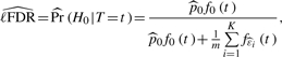
By utilizing our individual detectability estimates , we obtain an estimate of ℓFDR for a certain hypothesis (marker) as

(3)

where t is the test statistic value of the hypothesis, , and K is determined by the stopping rule. The exact value of ℓFDR is obtained by replacing with p₀=1−m₁/m and the individual detectability estimates with the real individual detectabilities in (3).

2.4 FDR

The frequently used approach to estimate q-values is based on the estimate of Pr(T ≥ t), i.e. the denominator in the exact q-value formula, by the corresponding empirical distribution function and some smoothing (Storey, 2002). In principle, a similar approach could be used to estimate ℓFDR, i.e. we could estimate the density function in the denominator in the formula that calculates the exact ℓFDR. However, approximating a density function by its empirical version is known to be inaccurate. Therefore, we use our individual detectability estimates instead, which provide us with an accurate estimate.

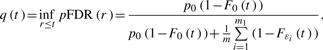
Note that we can estimate a q-value (Storey, 2002) in a similar fashion. The q-value of the observed test statistic value t is

(4)

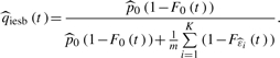
where ε₁,…, ε_m1 are the actual detectabilities. The reason why we can omit ‘inf’ is that the right-hand side in (5) is an increasing function of t when G_ε(p)/p≥g_ε(p), where G_ε(p) (g_ε(p)) is the distribution (density) function of p-value with detectability ε. It is reasonable to assume that G_ε(p)≥p, that is a p-value of an alternative hypothesis is more likely to fall in [0, p] than that of a null hypothesis. Then the condition G_ε(p)/p≥g_ε(p) typically holds, e.g. when G_ε(p) is concave [see (Storey, 2002) for further details]. By plugging our individual detectability estimates and into (5), we obtain a full parametric q-value estimate

(5)

Here, we can omit ‘inf’ for the same reason mentioned above. Note that the full parametric q-value estimate in (5) does not require smoothing. The smoothing results in equal q-value estimates that correspond to (sometimes quite many) consecutive p-values, although the real q-values corresponding to different p-values (often substantially) differ from each other.

3 RESULTS

3.1 Simulation results

In all simulations, test statistic values of true null hypotheses will be drawn from a central chi-squared distribution with 1 degree of freedom (d.f. 1). Alternative test statistic values will be drawn from a non-central χ²-distribution with d.f. 1 whose non-centrality parameter is the square of the detectability. For instance, this may be the approximating distribution for Pearson's statistic in allele-based case–control studies. Note that using a χ²-distribution is not critical here as our estimator would work equally well with other test statistic distributions.

In each simulation, we calculate the maximum difference (MD) between the function that assigns the true ℓFDR and the function that assigns the estimated ℓFDR to test statistic values. Note that the MD of a simulation represents the worst-case scenario as this is the maximum error that can occur between the real and estimated ℓFDR of a test statistic value. To show the direction of deviation of the estimated ℓFDR from the real one, we assign a negative sign to MD if the estimated ℓFDR is smaller than the real one at the point where the MD is taken. If the MD is positive, then the ℓFDR estimate is typically higher than the real ℓFDR in the entire region. Conversely, if the MD is negative then the ℓFDR estimate is typically lower than the real ℓFDR in the entire region.

In Figure 1, we plotted the true ℓFDRs (continuous line) and estimated ℓFDRs (dashed line) versus the −log₁₀ p-values. The log scale is used to ‘zoom in’ on the smaller p-values, which are more likely to represent markers related to the phenotype of interest. The log scale with basis 10 is also typically used for GWAS QQ plots. To create Figure 1, we used 500 replicates. For each replicate, we simulated 100 000 test statistic values, 10 of which had detectabilities equidistantly chosen from interval [4, 6], thus the detectabilities were 4.00, 4.22, 4.44, …, 5.78, 6.00. The estimated ℓFDRs were from the nine simulations whose MDs are the 10-quantiles in the 500 MDs. Figure 1 shows that our ℓFDR estimator is conservative in this condition, i.e. it overestimates ℓFDR suggesting a somewhat higher probability of a false positive, which is typical when the detectabilities are not high. The upward bias of our ℓFDR estimator is also reflected by the fact that the mean of the 500 MDs is positive, in particular it is 0.1. The ninth 10-percentile of the MDs is 0.199, which is the MD between the upper most dashed line and the solid line in the figure. Note that the difference between these two lines is typically <0.199, and even the MD was ≦0.199 in 90% of the 500 replicates. This means that in 90% of the cases, the MD between the real and estimated ℓFDR is <0.199, and typically much less even in these cases because the MD represents the worst-case scenario in every simulation. The 10-percentiles of MDs were 0.024 0.047 0.063 0.085 0.099 0.119 0.138 0.162 0.199.

Fig. 1.

The true ℓFDR (continuous line) and estimated ℓFDR (dashed lines) versus the −log₁₀ p-values are plotted. Each of the nine dashed lines is the estimated ℓFDR curve of one of the nine simulations selected from 500. The selected simulations were those whose MDs are the deciles of the MDs in the 500 simulations.

In Table 1, we examine the performance of our ℓFDR estimator through MDs for different number, range and distribution of positive detectabilities. In our baseline condition, the detectabilities are in the range 4.0–6.0. For instance, if in an allele-based case–control study we have 1000 cases and 1000 controls, then a marker with minor allele frequency 0.35 and odds ratio 1.3 (1.48) has detectability 4 (6). We examine three different type of distribution of detectabilities within a range. They are either equidistantly distributed (Equid) in the range when we have five detectabilities in the baseline condition, or concentrated to the endpoints (Conc Endp) of the range, i.e. half of them take one endpoint and the other half take the other endpoint. If we have an odd number of Conc Endp distributed positive detectabilities, then one of them equals the mean of the endpoints. For instance, five detectabilities in the range 4.0–6.0 can either take (4.0,4.5,5.0,5.5,6.0) or (4.0,4.0,5.0,6.0,6.0), which are Equid, and Conc Endp, respectively. We also examine scenarios where the baseline range, 4.0–6.0 is reduced to 80% (3.2–4.8) or increased to 120% (4.8–7.2). Note that the individual detectabilities are also reduced or increased by the given amount due to the specific patterns. In practice, the reduction to 80% of the detectabilities may mean reduction of the sample size to 64% while keeping the individual detectabilities the same. Conversely, the increase to 120% of the detectabilities may mean increase of the sample size to 144%. Finally, we vary the number of positive detectabilities, which may take 5, 10 or 20 in each condition. In order to provide better insight into the accuracy of the estimator, besides the mean and SD of the MDs, we also indicated the estimated radius of the zero-centered 90% CI of the MDs in the tables. Clearly, the radius of the CI is affected both by the mean and the SD of the MDs.

Table 1.

Mean, SD and the estimated radius (Conf) of zero-centered 90% confidence interval (90% CI) of the MDs between the real and estimated ℓFDR curves for different range, number and distribution of detectabilities (the number of markers was 100 000)

		Equid			ConcEndp
Range	#dets	Mean	SD	Conf	Mean	SD	Conf
3.2–4.8	5	0.207	0.26	0.599	0.149	0.23	0.335
	10	0.199	0.11	0.324	0.153	0.12	0.249
	20	0.225	0.07	0.314	0.184	0.07	0.267
4.0–6.0	5	0.060	0.11	0.188	0.029	0.09	0.137
	10	0.102	0.07	0.200	0.070	0.07	0.159
	20	0.126	0.06	0.207	0.123	0.05	0.190
4.8–7.2	5	−0.042	0.10	0.176	−0.022	0.10	0.169
	10	−0.008	0.08	0.136	0.055	0.09	0.194
	20	0.006	0.06	0.098	0.088	0.06	0.164

#dets = number of positive detectabilities.

The predominance of the positive mean MDs in Table 1 indicates the upward (conservative) bias of the ℓFDR estimator, i.e. it overestimates the ℓFDR. In particular, the mean of the MDs is higher for the lower range of positive detectabilities. Although, in most cases the mean of the MDs goes up slightly as the number of positive detectabilities gets larger, the mean of the MDs is mainly dependent on the range of the positive detectabilities. The mean of the MDs noticeably differs across the types of distributions of detectabilities when the range of the detectabilities is low (3.2−4.8). However, this difference becomes marginal for the higher range of detectabilities. Table 1 shows that the higher the number and the size of the positive detectabilities, the less the SD of the MDs. Moreover, the type of the distribution of the detectabilities has no substantial influence on the SD.

In Table 2, we increased the number of markers from 100 000 to 400 000, and kept all other conditions the same. Although, the proportion of positive detectabilities in the total set of markers is much smaller now, the estimator performed only slightly worse than for the same conditions in Table 1, indicated by the radius of the confidence interval. The exceptions are the lower range (3.2–4.8) and low number (5 or 10) of detectabilities.

Table 2.

Mean, SD and the estimated radius (Conf) of zero-centered 90% CI of the MDs between the real and estimated ℓFDR curves for different range, number and distribution of detectabilities (the number of markers was 400 000)

		Equid			ConcEndp
Range	#dets	Mean	SD	Conf	Mean	SD	Conf
3.2–4.8	5	0.256	0.33	0.965	0.231	0.32	0.927
	10	0.238	0.18	0.402	0.188	0.14	0.324
	20	0.246	0.08	0.350	0.210	0.07	0.299
4.0–6.0	5	0.091	0.12	0.211	0.062	0.11	0.182
	10	0.131	0.08	0.233	0.092	0.08	0.182
	20	0.158	0.06	0.240	0.132	0.06	0.210
4.8–7.2	5	−0.006	0.09	0.149	0.005	0.10	0.158
	10	0.032	0.08	0.138	0.072	0.08	0.177
	20	0.050	0.06	0.118	0.118	0.07	0.208

#dets = number of positive detectabilities.

In Table 3, we studied the performance of the ℓFDR estimator in the context of substantial correlation or linkage disequilibrium between the markers. The generated test statistic values were in LD within one block and uncorrelated between two different blocks. The blocks were equal in size, either 5 or 10. We simply used the correlation coefficient (square root of the r-squared, a frequently used measure of LD) with within-block correlation also equal, either 0.5, or 0.75 or 0.9. The other conditions were our (uncorrelated) baseline, which is also indicated in the first row of the table. The mean MD slightly changes across the different correlation structures, meaning that higher correlation results in a marginally higher bias. As one might expect, the higher the within-block correlation or the size of the block, the higher the SD. The changes in the mean and SD of the MDs are also reflected in the greater radius of the CI, although this change is not dramatic even in the extreme condition (within-block correlation 0.9, block size 10).

Table 3.

Mean, SD and the estimated radius (Conf) of zero-centered 90% CI of the MDs between the real and estimated ℓFDR curves for different correlation structures and number of detectabilities

		Five dets			20 dets
bs	cor	Mean	SD	Conf	Mean	SD	Conf
0	0	0.060	0.11	0.188	0.126	0.06	0.207
5	0.5	0.080	0.15	0.202	0.130	0.07	0.230
	0.75	0.103	0.21	0.247	0.136	0.09	0.260
	0.9	0.107	0.24	0.266	0.137	0.10	0.280
10	0.5	0.076	0.14	0.220	0.131	0.08	0.238
	0.75	0.099	0.22	0.259	0.137	0.12	0.278
	0.9	0.108	0.27	0.320	0.141	0.15	0.329

The number of markers was 100 000, moreover, 5, 10 or 20 of them had real detectabilities equidistantly chosen from [4.0,6.0] including the limits of the interval. dets = detectabilities, bs = block size, cor = block correlation.

In summary, the accuracy of the ℓFDR estimator is mainly dependent on the range and the number of the positive detectabilities. It only slightly depends on the total number of markers or on how the positive detectabilities are distributed, except for lower ranges of positive detectabilities, where the estimator is not precise anyway. The correlation structure has some but by no means dramatic influence on the performance of the ℓFDR estimator. We come to the same conclusion if median (MeD) rather than MD between the real and estimated ℓFDR curve is used (see Section 4 in Supplementary Material). However, the mean, SD and the estimated radius of zero-centered 90% CI of MeDs is substantially, often with an order of magnitude, less than that of the MDs.

The running time of the ℓFDR estimator ranged 1–4 min and 10–50 s when R code and C++ code was used, respectively, on a desktop computer with 2.4 GHz dual core processor and 2.00 GB RAM for numerical examples with 400 000 hypotheses/markers, where 10 of them were true alternatives. The running time mainly depends on these two factors.

3.2 Application to GWAS for neuroticism

We will illustrate our method on GWAS data for Neuroticism which are available from the NIMH Genetics repository. Neuroticism, a personality trait reflecting a tendency towards negative mood states (Costa and McCrae, 1980), is a risk factor for psychiatric conditions such as anxiety and depression (Brandes and Bienvenu, 2006; Widiger and Trull, 1992). Details of this study can be found elsewhere (van den Oord et al., 2008). In short, the GWAS sample consisted of healthy subjects ascertained from a US national sampling frame. The genotype data were generated at the Center for Genotyping & Analysis at the Broad Institute of Harvard and MIT. The Affymetrix 500K ‘A’ chipset (www.affymetrix.com/support/technical/datasheets/500k_datasheet.pdf) was used and genotypes were called using the Affymetrix BRLMM algorithm. Quality control (QC) analyses resulted in the exclusion of samples (e.g. samples achieving a Single Nucleotide Polymorphism (SNP) call rate of <95% and individuals with unusual degrees of relatedness or heterozygosity) and SNPs (e.g. we excluded SNPs with >10% missing genotypes, minor allele frequencies <0.005, showing extreme deviations from Hardy–Weinberg Equilibrium and SNPs on the sex chromosomes). After QC, a sample of 1227 subjects genotyped for 420 287 SNPs remained. Regression analyses were used to test whether individual SNPs were associated with neuroticism, where covariates were included to regress out the effects of ancestral background.

According to Meinshausen–Rice's p₀ estimator with fine-tuning parameter α=0.5, the number of positive effects/detectabilities is 6.48. Following our rule we, therefore, stop estimating effects at K=7.

Table 4 shows that the ℓFDR estimate of the marker with the highest test statistic value is 0.508, meaning that the probability that this marker has no effect given its test statistic value is ∼0.508. The q-value estimate that corresponds to this marker is 0.257 according to Storey's estimator. Note that this q-value estimate is considerably lower than the ℓFDR estimate of 0.508. An explanation is that the smallest q-value is the average probability (=FDR) of all hypothetical markers in the entire rejection region and that the probability of being a false positive is always higher for the marker with the largest test statistic. Also note that Storey's q-value estimates are the same for all eight markers. This is the result of the estimation procedure that forces estimated q-values to be equal or smaller for decreasing p-values. In contrast, the full parametric q-value estimator in (5) does not have that property.

Table 4.

ℓFDR and q-value estimates of the eight markers with the highest test statistic value in neuroticism data

	CHR ID*	SNP ID	ℓFDR est.	STO	FPQ
1	14	rs2416009	0.508	0.257	0.212
2	14	rs12883384	0.536	0.257	0.229
3	14	rs1959813	0.539	0.257	0.231
4	14	rs7151262	0.566	0.257	0.249
5	8	rs2936594	0.600	0.257	0.274
6	8	rs1877332	0.647	0.257	0.311
7	7	rs17773605	0.754	0.257	0.417
8	10	rs7080041	0.805	0.257	0.483

The q-values were calculated by Storey's method as well as by the full parametric q-value estimate. STO = Storey's q-value estimate, FPQ = full parametric q-value estimate.

*CHR ID=chromosome ID

4 DISCUSSION

A limitation shared by multiple methods used to declare significance in GWAS is that they do not provide clear information about the probability that GWAS findings are true or false. This lack of information increases the chance of false discoveries and may result in real effects being missed. To better evaluate GWAS findings and improve the subsequent selection of markers for further studies, we propose a method to estimate the posterior probability that a marker has (no) effect given its test statistic value, also called ℓFDR, in the GWAS. Such posterior probabilities are notoriously difficult to estimate precisely. The estimator proposed in this article remedies this precision problem by taking advantage of the facts that in GWAS good approximations of the test statistic distribution often exist and that the number of markers with effects is likely to be small. At the heart of our method is the estimation of the (detectability) parameters of the densities under the alternative for which we use the real maximum likelihood function rather than the mixture model maximum likelihood function. Simulations show that our estimator provides accurate ℓFDR estimates. This accuracy is mainly dependent on the size, range and the number of detectability parameters. The LD between the SNPs has some, but much more modest, influence on the precision of the estimates. GWAS data are used to illustrate differences of ℓFDR versus traditional FDR methods empirically.

A first step in our method is to estimate the individual detectability parameters of the densities under the alternative distributions. The detectability parameter equals the square root of the sample size times the effect size of the marker. The detectability estimates are then used in the second step to calculate the ℓFDR estimates. It is important to stress that our detectability estimates are obtained using information from the entire set of tested markers and not just those markers that are declared significant. Therefore, unlike existing approaches that estimate the effect sizes of only the significant markers in the same sample that has been used for testing, our detectability estimator cannot suffer from the upward bias associated with this approach (Goring et al., 2001; Ioannidis et al., 2001).Furthermore, no assumptions are made about the distribution of the individual detectabilities. This is important because it will be almost impossible to justify parametric assumptions about this distribution in genetic association studies.

Our proposed method for estimating ℓFDR can be used in all scenarios where the distribution under the alternative hypotheses can be characterized by a single value. This is the case for the vast majority of tests performed in statistical genetics. For example, categorical tests, quantitative tests, case–control tests and tests used in the context of family based designs typically have either a non-central χ² or non-central F-distributions under the alternative that depend on a single parameter only. In addition, statistics used to test for interactions or more complex models also typically have single value approximations under the alternative (e.g. Wald test for the significance of the interaction effect or likelihood ratio tests obtained by fitting multiple/logistic regression models with and without the interaction effects). Thus, our approach is very general and can be used in a wide variety of scenarios.

Several extensions of our method are conceivable. For example, because markers with very small effects should have somewhat larger test statistic values than true nulls, they will still get a somewhat higher estimated ℓFDR. However, it is unlikely that markers with effect sizes that would be hard to detect in association studies, would get noticeably better estimated ℓFDR. Although, it will be impossible to estimate the potentially many very small effects individually, it may be possible to devise a method that estimates the average of all the undetectable effect sizes simultaneously. This group estimate could then be used to estimate the posterior probability that individual markers belong to this group. A second possible extension will be to calculate posterior probabilities after imputing missing SNPs. The imputation of SNPs alters the distribution of the test statistic as a result of the uncertainty in inferring the unknown variants. By approximations of the adjusted test statistic distributions, as for instance, proposed by (Lin et al., 2008), we can calculate posterior probabilities for imputed SNPs.

In this article we illustrated the use of ℓFDRs for the evaluation of GWAS results and to improve subsequent marker selection. Several other applications of the estimated ℓFDRs are conceivable. For example, geneticists may be interested in combining markers in specific biological pathways or genomic (linkage) regions to test whether an entire pathway or region is more likely to be associated with the outcome of interest. Marker-specific information is needed to combine evidence in the pathway or region. Because FDR-based statistics such as q-values do not provide marker-specific information, they cannot be used in such scenarios where markers are selected for reasons other then having p-values below a certain threshold. The ℓFDRs do, however, provide marker specific information, and therefore provide the prospect of testing for enrichment of biological pathways and regions for disease signals. A final example of how the estimated posterior probabilities can be used involves replication studies. Posterior probabilities provide an estimate for the amount of prior evidence that a specific marker will replicate. As such more powerful replication studies could be designed by giving more weight to markers that have higher prior probabilities of being true. Moreover, current rules for declaring significance in replication studies tend to be somewhat arbitrary (e.g. p-values < 0.05 suggest a replication). Using the posterior probabilities estimated from the GWAS data as prior probabilities in replication studies could in principle help interpret results of replication studies and define more statistically motivated decision rules for declaring significance.

REFERENCES

- Allison DB, et al. A mixture model approach for the analysis of microarray gene expression data. Comput. Stat. Data Anal. 2002;39:1–20. [Google Scholar]
- Aubert J, et al. Determination of the differentially expressed genes in microarray experiments using local fdr. BMC Bioinformatics. 2004;5:125. doi: 10.1186/1471-2105-5-125. [DOI] [PMC free article] [PubMed] [Google Scholar]
- Benjamini Y, Hochberg Y. Controlling the false discovery rate: a practical and powerful approach to multiple testing. J. R. Stat. Soc. B. 1995;57:289–300. [Google Scholar]
- Benjamini Y, Hochberg Y. On adaptive control of the false discovery rate in multiple testing with independent statistics. J. Edu. Behav. Stat. 2000;25:60–83. [Google Scholar]
- Black MA. A note on the adaptive control of false discovery rates. J. R. Stat. Soc. B. 2004;66:297–304. [Google Scholar]
- Brandes M, Bienvenu OJ. Personality and anxiety disorders. Curr. Psychiatry Rep. 2006;8:263–269. doi: 10.1007/s11920-006-0061-8. [DOI] [PubMed] [Google Scholar]
- Costa P.TJ, McCrae RR. Influence of extraversion and neuroticism on subjective well-being: happy and unhappy people. J. Pers. Soc. Psychol. 1980;38:668–678. doi: 10.1037//0022-3514.38.4.668. [DOI] [PubMed] [Google Scholar]
- Dalmasso C, et al. A simple procedure for estimating the false discovery rate. Bioinformatics. 2005;21:660–668. doi: 10.1093/bioinformatics/bti063. [DOI] [PubMed] [Google Scholar]
- Dalmasso C, et al. A constrained polynomial regression procedure for estimating the local false discovery rate. BMC Bioinformatics. 2007;8:229. doi: 10.1186/1471-2105-8-229. [DOI] [PMC free article] [PubMed] [Google Scholar]
- Efron B, et al. Empirical bayes analysis of a microarray experiment. J. Am. Stat. Assoc. 2001;96:1151–1160. [Google Scholar]
- Finner H, Roters M. On the false discovery rate and expected type i errors. Biometr. J. 2001;8:985–1005. [Google Scholar]
- Glonek G, Soloman P. Discussion of resampling-based multiple testing for microarray data analysis by ge, dudoit and speed. Test. 2003;12:1–77. [Google Scholar]
- Goring H.HH, et al. A revised version of the psychoticism scale. Am. J. Hum. Genet. 2001;69:1357–1369. doi: 10.1086/324471. [DOI] [PMC free article] [PubMed] [Google Scholar]
- Ioannidis JP, et al. Replication validity of genetic association studies. Nat. Genet. 2001;29:306–309. doi: 10.1038/ng749. [DOI] [PubMed] [Google Scholar]
- Liao JG, et al. A mixture model for estimating the local false discovery rate in dna microarray analysis. Bioinformatics. 2004;20:2694–2701. doi: 10.1093/bioinformatics/bth310. [DOI] [PubMed] [Google Scholar]
- Lin DY, et al. Simple and efficient analysis of disease association with missing genotype data. Am. J. Hum. Genet. 2008;82:444–452. doi: 10.1016/j.ajhg.2007.11.004. [DOI] [PMC free article] [PubMed] [Google Scholar]
- Meinshausen N, Rice J. Estimating the proportion of false null hypotheses among a large number of independently tested hypotheses. Ann. Stat. 2006;34:373–393. [Google Scholar]
- Ploner A, et al. Multidimensional local false discovery rate for microarray studies. Bioinformatics. 2006;22:556–565. doi: 10.1093/bioinformatics/btk013. [DOI] [PubMed] [Google Scholar]
- Pounds S, Morris SW. Estimating the occurrence of false positives and false negatives in microarray studies by approximating and partitioning the empirical distribution of p-values. Bioinformatics. 2003;19:1236–1242. doi: 10.1093/bioinformatics/btg148. [DOI] [PubMed] [Google Scholar]
- R Development Core Team. R: A Language and Environment for Statistical Computing. Vienna, Austria: R Foundation for Statistical Computing; 2008. [Google Scholar]
- Scheid S, Spang R. A stochastic downhill search algorithm for estimating the local false discovery rate. EEE Trans. Comput. Biol. Bioinform. 2004;1:98–108. doi: 10.1109/TCBB.2004.24. [DOI] [PubMed] [Google Scholar]
- Storey JD, Tibshirani R. Statistical significance for genome-wide studies. Proc. Natl Acad. Sci. 2003;100:9440–9445. doi: 10.1073/pnas.1530509100. [DOI] [PMC free article] [PubMed] [Google Scholar]
- Storey JD, et al. Strong control, conservative point estimation and simultaneous conservative consistency of false discovery rates: a unified approach. J. R. Stat. Soc. B. 2004;66:187–205. [Google Scholar]
- Storey JD. A direct approach to false discovery rates. J. R. Stat. Soc. B. 2002;64:479–498. [Google Scholar]
- Storey JD. The positive false discovery rate: A bayesian interpretation and the q-value. Ann. Stat. 2003;31:2013–2035. [Google Scholar]
- van den Oord EJ, et al. Genomewide association analysis followed by a replication study implicates a novel neuroticism gene. Arch. Gen. Psychiatry. 2008;65:1062–1071. doi: 10.1001/archpsyc.65.9.1062. [DOI] [PubMed] [Google Scholar]
- Widiger TA, Trull TJ. Personality and psychopathology: an application of the five-factor model. J. Pers. 1992;60:363–393. doi: 10.1111/j.1467-6494.1992.tb00977.x. [DOI] [PubMed] [Google Scholar]
- Zaykin DV, Zhivotovsky LA. Ranks of genuine associations in whole-genome scans. Genetics. 2005;171:813–823. doi: 10.1534/genetics.105.044206. [DOI] [PMC free article] [PubMed] [Google Scholar]