Detecting Change in Biological Rhythms: A Multivariate Permutation Test Approach to Fourier-Transformed Data

Abstract

Treatment-related changes in neurobiological rhythms are of increasing interest to psychologists, psychiatrists, and biological rhythms researchers. New methods for analyzing change in rhythms are needed, as most common methods disregard the rich complexity of biological processes. Large time series data sets reflect the intricacies of underlying neurobiological processes, but can be difficult to analyze. We propose the use of Fourier methods with multivariate permutation test (MPT) methods for analyzing change in rhythms from time series data. To validate the use of MPT for Fourier-transformed data, we performed Monte Carlo simulations and compared statistical power and family-wise error for MPT to Bonferroni-corrected and uncorrected methods. Results show that MPT provides greater statistical power than Bonferroni-corrected tests, while appropriately controlling family-wise error. We applied this method to human, pre-and post-treatment, serially-sampled neurotransmitter data to confirm the utility of this method using real data. Together, Fourier with MPT methods provides a statistically powerful approach for detecting change in biological rhythms from time series data.

Introduction

Treatment-related changes in neurobiological rhythms are of increasing interest. However, characterizing changes in biological rhythms can be challenging. Rhythmic patterns in time series data can be extracted by spectral analytic methods like Fourier-transforms, but statistical methods are needed to compare rhythms within subjects. Common methods for analyzing time series data compress information to only a small number of values (e.g., Matthews et al., 1990), which rarely represent the complexity of biological rhythms. Although data sets comprised of many measurements improve the description of complex processes, performing multiple statistical tests introduces problems. For instance, the statistical comparison of many data points (i.e., multiple testing) increases family-wise error, which is the probability of finding at least one false positive out of a set, or “family,” of related research questions. The most common method for controlling family-wise error is the Bonferroni correction (Bonferroni, 1936), which is often overly conservative (Perneger, 1998). In this paper, we assess the use of multivariate permutation tests (Blair & Karniski, 1993; Troendle, 1995; Westfall & Young, 1993) for controlling family-wise error in an analysis of medication treatment effects on Fourier-transformed biological rhythms.

A desire to test for antidepressant treatment effects on rhythmicity in neurotransmitter levels in depression motivated this study. Neurotransmitters, such as serotonin, norepinephrine, and dopamine, are implicated in the pathophysiology of depression, and antidepressant medications and other treatments that target neurotransmitter function both restore normalcy of peripherally measured rhythms (Benedetti et al., 2007; Souetre et al., 1989) and improve depressive symptoms (Benedetti et al., 2007; Loosen et al., 2000). A study of cerebrospinal fluid was conducted in a small number of patients to examine the effect of antidepressant treatment on neurotransmitter rhythms through a 24 h cycle. The study estimated the impact of antidepressant treatment on neurotransmitter-level rhythms at different times of day. Common methods for comparing spectra, such as comparing peak intensities (of domain frequencies) and cross-spectral analyses (Warner, 1998), were inadequate because they only compare global qualities of the spectral findings. Uncorrected paired t-tests on each of the frequencies throughout the day (n = 930) would have produced Type I error rates larger than our specified α = .05, while Bonferroni-correction methods would be overly conservative.

Multivariate permutation tests (MPT) compute statistical significance for large numbers of tests while controlling family-wise error rates (Blair et al., 1994; Pesarin, 2001; Westfall & Young, 1993). In the remainder of this article, we describe standard Fourier transformations and MPT methods. We then report results from a simulation study testing the application of MPT to Fourier-analyzed data, and compare MPT to more traditional methods for controlling family-wise error. Finally, we demonstrate the application of MPT methods using a previously published data set (Salomon et al., 2005)

Fourier Analyses

Analysis of time series data in the time domain provides a global measure of changes in a signal (e.g., trend analysis). In contrast, frequency domain approaches using spectral analysis (e.g., harmonics) detect rhythmic patterns. One type of spectral analysis, Fourier analysis, identifies periodic patterns by partitioning the data into individual sinusoidal signals of different frequencies (Shumway & Stoffer, 2006; Warner, 1998). Fourier analyses are widely accepted as the best expression of regularity of a time series (Shumway & Stoffer, 2006).

Origins of Fourier analysis can be traced to a series of papers on heat transfer by Jean Baptiste Joseph Fourier (1768–1830). In these papers, Fourier demonstrated that naturally occurring time series could be decomposed into a unique set of independent sine waves in which each wave is defined by an amplitude and frequency parameter. The weighted sum of these component waves reconstructs the original composite time series. Fourier coefficients are simply the amplitudes of the sine waves at each frequency. The introduction of efficient algorithms for computing Fourier coefficients (Cooley & Tukey, 1965) and high-speed computers have made Fourier analysis an accessible and powerful method for analyzing time structured data (see Figure 1). The application of Fourier analysis to subsets of data, or sequential windows in the time series, produces a spectrogram (i.e., a two-dimensional matrix of Fourier coefficients arranged by time and frequency). In contrast to a periodogram—which uses single Fourier analysis to provide a single set of coefficients in the frequency domain—spectrograms present a series of frequency coefficients over time.

Figure 1.

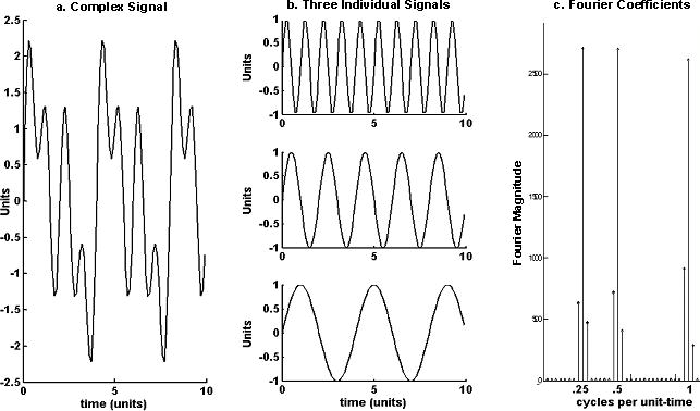
Decomposition of a complex signal. A complex signal (a) is decomposed into three individual signals (b) with frequencies (cycles per time unit) of 0.25, 0.5, and 1, respectively. Fourier coefficients (c) show the three distinct frequencies which contribute to the complex signal. The smaller coefficients flanking the main peaks are common artifacts referred to as “lobes.”

Analytic Challenges

Large numbers of coefficients from Fourier transforms present a challenge for statistical testing. Fourier coefficients are neither normally distributed (Shumway & Stoffer, 2006, pp. 280–281) nor independent, two central assumptions for parametric statistics. Although some parametric statistics are robust to minor violations of normality, nonparametric statistics can have greater power to detect group differences in highly skewed data (e.g., Blair & Higgins, 1980; Chernoff & Savage, 1958; Hodges & Lehmann, 1956). For example, in tests of paired samples using a chi-square distribution (df = 1), the Wilcoxon Signed Rank (WSR) test shows a consistent power advantage over the paired samples t test (Blair & Higgins, 1985). Nonparametric statistics can be performed on non-normal data; however, the issue of independence would still remain. Some methods exist to reduce the dependency, or correlations, between Fourier coefficients (Shiavi, 2006), but these are only partially successful.

The multivariate permutation test (MPT) controls family-wise error and does not require data normality or independence. Moreover, past research suggests this approach has greater statistical power than standard multiple comparison methods (Blair et al., 1996; Karniski et al., 1994; Yoder et al., 2004), especially when there are multiple dependent outcome variables. In the next section, we describe the underlying logic of univariate permutation tests followed by a description of the extension to multiple outcome variables, the multivariate permutation test.

Permutation Tests

Permutation tests represent a simple and intuitive method for determining significance levels for a statistical test (Edgington, 1995; Fisher, 1935, 1966;Good, 2000; Pitman, 1937, 1938), without assumptions of normal data distributions. Permutation tests use the study data to create an empirical distribution of test statistic values under the null hypothesis. For example, for treatment studies, the null hypothesis is often that the data are random observations from a population with no treatment-related differences. With two observations per subject, under the null hypothesis, we expect the pre- and post-treatment observations to be equivalent, with any individual differences randomly distributed between the two time points. To create a null hypothesis distribution, each subject’s data are randomly assigned to either the pre- or post-treatment condition, and a test statistic (e.g., t value) is computed and recorded. This process is repeated many times. The aggregate of these statistics defines a distribution of the test statistic under the null hypothesis of no treatment effect. Using this distribution, a p value is computed as the probability of observing a test statistic as extreme as or more extreme than the observed test statistic.

Although permutation tests do not require normal data distributions, observations must be exchangeable. Exchangeability means that the observations are equivalent and can be substituted across groups. That is, “under the null hypothesis of no differences among the various experimental or survey groups, can we exchange the labels on the observations without affecting the results?” (Good, 2000). Independent observations from equal distributions are exchangeable. Examples of situations where data will not be exchangeable are confounding variables or differences in error variance (between groups or time points).

Multivariate Permutation Tests

MPT extends permutation tests to multiple outcome variables using three modifications. First, MPT simultaneously permutes all outcome variables as a single set, thereby preserving their natural correlations. Second, a multivariate statistic (e.g., the largest absolute t) is used to produce a single statistic value for each permutation. Third, a “step-down” procedure (Hochberg, 1988; Holm, 1979) controls for family-wise error by incrementally relaxing the significance criterion following each significant result (Blair & Karniski, 1994). A step-by-step description of the MPT method is provided in Table 1.

Table 1.

Multivariate permutation test methods

Specify the research question.

Are there pre–post differences on any of the 72 Fourier coefficients?

State the null hypothesis.

There are no pre–post differences for any of the 72 Fourier coefficients.

Chose a test statistic.

A paired t-test was used to compare the within-subjects (pre–post) measures.

Compute the test statistic for each of the observed data points.

Difference scores were computed for each of the 72 data points for each subject. T-tests were computed for each of the 72 variables, comparing the average difference score with a difference score of 0. These were the “observed” test statistics.

Rearrange the observations by randomly shuffling the experimental factor (treatment).

Each subject had a row of data comprised of the difference score for each of the 72 variables. The null hypothesis of no treatment effect was created by randomly assigning a positive (+) or (−) sign for each subject. Each permutation was implemented by randomly applying a positive (+) or negative (−) sign to all 72 Fourier coefficient difference scores (post–pre) for each subject, effectively removing any true treatment effect. By randomly applying the signs across subjects, any true treatment effects were nullified, while maintaining the distribution of absolute values. Application of the sign (+/−) across all of the data points for a single subject preserved the natural correlations among variables.

Compute the test-statistic for each of the dependent variables for the newly arranged data.

Once the signs of the difference scores have been changed, new t values were computed for each of the 72 variables.

Select a multivariate statistic to summarize across the outcome variables and save the value of that statistic.

The largest absolute t value across all outcome variables was identified, and this single value was saved.

Continue to rearrange the observations and compute the multivariate test statistic many times.

The rearrangement process was conducted 1,000 times. The largest absolute t value was saved each time and formed the distribution of the test statistics under the null hypothesis.

Sort the observed t values from all of the outcome variables and perform significance tests.

The t values for all 72 Fourier coefficients were sorted in descending order. A p value was computed as the probability of observing a test (t) statistic as extreme as or more extreme than the observed test (t) statistic.

Use a step-down process to test remaining variables.

A step-down process was then used to iteratively test the significance of each of the outcome variables until the first non-significant result was obtained. If the p value was ≤ .05, all Fourier coefficients for that frequency were removed from both the distribution and original data set. Repeating the permutation process created a new distribution. This significance testing process continued until the p value was > .05 for a given Fourier coefficient. All remaining t values were considered not significant. This permutation method provided significance results (i.e., significant/non-significant) for each of the 72 Fourier frequencies in each experiment.

MPT methods were introduced independently by Troendle (1995), Westfall and Young (1993), and Blair and Karniski (1993), and have been discussed elsewhere in detail (Blackford, 2007; Pesarin, 2001). MPT methods have been used successfully to test within-subjects differences in frequent and rare auditory waveform potentials (Blair & Karniski, 1993) and dipole separation (Karniski et al., 1994). Yoder and colleagues (2004) used MPT to test correlations between voxels from an electroencephalogram and various behavioral measures. To our knowledge, the current study is the first evaluation of MPT for Fourier coefficients.

In summary, we suggest that the understanding of medication treatment effects will be increased by examining multiple measurements representing biological rhythms instead of global summary measures from a time series. We identify MPT as a possible statistical method for significance testing of treatment effects in Fourier-derived multiple rhythm measures because MPT methods can be used on non-normal, correlated data and have been shown to provide good family-wise error protection for other types of data. To test the performance of MPT methods for significance testing, we conducted a simulation study comparing MPT to two standard methods, multiple tests with and without Bonferroni corrections. We chose the paired t-test as the primary statistic for the simulation study because the t-test is commonly used to test for within-group differences and the implementation of MPT for paired t-tests has been previously described (Blair & Karniski, 1994; Edgington, 1995). To provide a comprehensive test of MPT, we also used a second nonparametric statistic, the WSR test, for the two standard significance testing methods. We hypothesized that for Fourier-transformed time series data, MPT would have more statistical power than the Bonferroni correction and would better control family-wise error (to the specified a) than either the Bonferroni-corrected or uncorrected method.

Simulation Study

Materials and Methods

Overview

We used simulation methods to compare statistical power and family-wise error for three methods of determining statistical significance for the paired t-test: MPT, Bonferroni-corrected tests, and uncorrected tests. The Bonferroni and uncorrected methods were also tested for the WSR test statistic. We used each method to test the significance of Fourier coefficients for three sample sizes (10, 20, and 30) and seven levels of treatment effect (10–40%, in 5% increments). For each combination of method, sample size, and treatment effect, we performed 5,000 experiments. The R statistical software (http://www.r-project.org; version 2.5.1; R Development Core Team, 2007) was used for all simulations and statistical analyses. The R fft function (R Stats package) computed Fast Fourier Transforms, and a custom-written program performed the MPTs (see Appendix; also available at http://www.blackfordlab.com/publications/).

Data Simulation

We simulated the time series data for this study because known treatment effect values are required for measurement of statistical power and Type I error. We chose the sinusoid to model periodic data because this basic waveform provides well-defined Fourier coefficients, allowing precise specifications of treatment effects. To test for both statistical power and Type I error within a single simulation study, the model must include both signals that show change (to test for power to detect a treatment effect) and signals that are unchanged (to test for Type I error when there is no treatment effect). Therefore, a complex signal was modeled by summing three independent sinusoids of 144 time points, but only one of the sinusoids became more powerful in the post-treatment signal. A treatment effect (T_e) was modeled by increasing the amplitude of the sinusoid in the post-treatment signal by one of seven amounts (T_e = 1.10–1.40, in .05 increments). The pre- and post-treatment signals were as follows:

$$\text{Pre}-\text{treatment}\text{signal}(i)=sin(.2i)+sin(.8i)+sin(1.5i)$$

$$\text{Post}-\text{treatment}\text{signal}(i)=sin(.2i)+({\text{T}}_{\text{e}}\times sin(.8i))+sin(1.5i)$$

where i runs from 1, 2, … , 144. Normally distributed (μ = 0, σ² = 1), random noise time series were added to each subject’s pre- and post-treatment signals. The signal plus noise time series were transformed using a Fast Fourier Transform and a Hanning filter (Blackman & Tukey, 1959) to produce 72 Fourier coefficients for each treatment time (pre/post) and subject.

Significance Test Methods

For the two standard significance testing methods, both paired t and WSR statistics were used. In the uncorrected test condition, p values were determined using standard distributions (Student’s t or WSR) and were not adjusted for multiple testing. The Bonferroni correction condition also used the standard distributions, but the α level was adjusted using the Bonferroni method (i.e., p value/number of tests). For the multivariate permutation test condition, permutation methods (see Table 1) for paired data (Edgington, 1995) were applied to the Fourier coefficients. The permutation consisted of 1,000 data rearrangements and used the largest absolute t value across the 72 Fourier coefficients to form the test distribution. A step-down significance testing process iteratively assessed statistical significance for the Fourier coefficients.

Outcome Measures

Statistical power, family-wise error rate, and effect size were computed from the results of 5,000 experiments for each study condition (i.e., sample size by treatment effect). We modeled treatment effects as the percent increase in the amplitude of the signal to provide a standard metric across samples sizes. The largest Fourier coefficient represented the treatment effect, and all other coefficients represented no treatment effect. As is standard in Monte Carlo simulations of this type (Mooney, 1997), statistical power was computed as the percentage of experiments for which the true treatment effect was statistically significant. Family-wise error rates were computed as the percentage of coefficients previously defined as “no treatment effect” that were statistically significant (i.e., Type I error). Statistical power across conditions was summarized using medians and interquartile ranges, because the values were not normally-distributed. Effect size, Cohen’s d (Cohen, 1992), for dependent groups was computed from the observed t value, corrected for correlations across pairs of measures:

$$d=t\sqrt{\frac{2(1-r)}{n}},$$

where r is the correlation between the two dependent measures (Dunlap et al., 1996). Effect size estimates were averaged across experiments to provide a standard measure of treatment effects.

Results

Comparisons of statistical power and family-wise error rates revealed significant differences among three (MPT/Bonferroni/uncorrected) methods used for estimating statistical significance for Fourier coefficients. The method differences varied by statistic, effect size, and sample size, as described below.

Statistical Power

The MPT method had greater statistical power than the Bonferroni-correction for both the t and WSR statistics (see Table 2). Across sample sizes and treatment effect levels, power was higher for the MPT compared to Bonferroni method for both the t statistic (16%; 69% vs. 53%) and WSR statistic (23%; 69% vs. 46%). The increase in power for the MPT relative to the Bonferroni method was the same or higher for the WSR than the t statistic for every combination of sample size and effect size.

Table 2.

Median statistical power by sample size, effect size, and statistic

			t-test			WSR
Sample size	Percent change	Effect size	MPT	Bonferroni	Uncorrected	Bonferroni	Uncorrected
10	10%	0.5	0.02	0.01	0.24	0.00	0.22
10	15%	0.7	0.06	0.03	0.49	0.00	0.45
10	20%	1.0	0.15	0.08	0.72	0.00	0.68
10	25%	1.2	0.30	0.19	0.88	0.00	0.85
10	30%	1.5	0.49	0.33	0.96	0.00	0.95
10	35%	1.7	0.69	0.53	0.99	0.00	0.99
10	40%	2.0	0.83	0.71	1.00	0.00	1.00
Median (IQR)			0.30 (0.63)	0.19 (0.50)	0.88 (0.50)	0.00 (0.00)	0.85 (0.54)
20	10%	0.7	0.08	0.05	0.48	0.04	0.43
20	15%	1.0	0.29	0.21	0.82	0.18	0.77
20	20%	1.3	0.61	0.52	0.97	0.46	0.95
20	25%	1.7	0.87	0.80	0.99	0.76	1.00
20	30%	2.0	0.98	0.96	0.99	0.94	1.00
20	35%	2.3	1.00	1.00	1.00	0.99	1.00
20	40%	2.6	1.00	1.00	1.00	1.00	1.00
Median (IQR)			0.87 (0.71)	0.80 (0.79)	0.99 (0.18)	0.76 (0.81)	1.00 (0.23)
30	10%	0.8	0.17	0.13	0.68	0.12	0.62
30	15%	1.2	0.57	0.49	0.95	0.47	0.94
30	20%	1.6	0.89	0.85	1.00	0.83	1.00
30	25%	2.0	0.99	0.99	1.00	0.98	1.00
30	30%	2.4	1.00	1.00	1.00	1.00	1.00
30	35%	2.8	1.00	1.00	1.00	1.00	1.00
30	40%	3.2	1.00	1.00	1.00	1.00	1.00
Median (IQR)			0.99 (0.43)	0.99 (0.51)	1.00 (0.05)	0.98 (0.53)	1.00 (0.06)

Note. Percent change is the targeted within-subjects treatment effect. Effect size is a standardized expression of this treatment effect.

The power advantage of MPT differed by effect size and sample size (see Figure 2). For very large effects (d ≥ 2), there was a ceiling effect where all methods had high power. For effect sizes less than two, the MPT power advantage increased as effect sizes became larger. The increase in statistical power for the MPT was greatest for the small sample size (N = 10), averaging across all effect sizes. For the t statistic, the power advantage for the MPT compared to the Bonferroni correction for the small, medium, and large samples were 11% (30% vs. 19%), 7% (87% vs. 80%), and 0% (99% vs. 99%), respectively, across all effect sizes (see Table 2). These differences were more notable for the WSR statistic, reaching 30% (30% vs. 0%), 11% (87% vs. 76%), and 1% (99% vs. 98%), respectively. As expected, statistical power for the uncorrected method was higher than the MPT method (30%; 99% vs. 69%). However, this increase came at the expense of substantially higher family-wise error.

Figure 2.

Statistical power curves by sample size. Statistical power curves for MPT, Bonferroni-corrected t, and Bonferroni-corrected WSR statistics by effect size (d). Shown are sample sizes of 10, 20, and 30.

Family-wise Error

Family-wise error rates followed the hypothesized directions for the three methods. Effect size had little impact on family-wise error rates across all methods; therefore, results are presented by sample size only (see Table 3). For the uncorrected tests, high (>.85) family-wise error rates indicated that most of the statistically significant findings were erroneous. The Bonferroni-corrected tests were overly conservative; that is, family-wise error rates were smaller than the specified a (0.05). For the MPT method, family-wise error rates were at, or close to, the specified α of .05 across all sample sizes and effect sizes. The consequence of increasing sample size was very small, and only observed for the WSR statistic (both Bonferroni-corrected and uncorrected).

Table 3.

Family-wise error by sample size and statistical test

	t-test			WSR
Sample size	MPT	Bonferroni	Uncorrected	Bonferroni	Uncorrected
10	0.04	0.01	0.94	0.00	0.90
20	0.05	0.02	0.95	0.03	0.87
30	0.05	0.02	0.95	0.04	0.86

To summarize our simulation results, the MPT method had greater statistical power than the Bonferroni-correction, while appropriately controlling family-wise error.

Practical Application

An application of MPT to real data demonstrates the utility of our findings. We compared the performance of the three aforementioned methods using data from the Salomon et al. (2005) study that motivated this work. The researchers hypothesized that antidepressant treatment would change neurotransmitter rhythms.

Materials and Methods

Subjects and Methods

Thirteen subjects (nine female) diagnosed with a major depressive episode were studied both before and after antidepressant medication treatment. Subjects were 25 to 60 yrs of age (mean 37.7). Studies were conducted with one subject at a time, throughout the annual cycle, and women were scheduled to coincide with their follicular phase. The 24 h cerebrospinal fluid (CSF) sampling sessions began on Thursdays at 08:00 h following a 12 h supine span and with placement of a lumbar catheter at 07:00 h.

The room was equipped as a standard medical hospital room. Subjects were confined to a bed that was kept flat throughout the study with only one pillow, with frequent repositioning and freedom of movement allowed. Subjects could listen to music through headphones, watch television, or read (except for materials with highly emotional or frightening content), and daytime naps were discouraged. Visitors were allowed during the day for up to 1 h. The room was illuminated with sun and standard fluorescent lighting and darkened with opaque window treatments. Lights were turned off from 22:30 h to 06:00 h with minimal lighting allowed for catheter maintenance or sample handling. Tympanic temperature was measured every 2 h while the subject was awake and also at 02:00 h.

Monoamine-balanced, caffeine-free diets were controlled for 72 h prior to study. Nutrition was limited to selections from standard hospital menus at 06:30 h (breakfast) and 09:30 h (lunch) with no supper to minimize ultradian nutrient fluctuations. Continuous hydration was maintained with D5W intravenously at 125 ml/h, and water was allowed ad libitum. No medications were administered during CSF collections except for continuing the antidepressant medication during the second study session. There were no adverse effects during collections, but half of the catheterizations resulted in moderate to severe post-puncture headaches, all of which resolved.

Serotonin and dopamine metabolite levels were determined by HPLC in 1 ml samples collected every 10 min by a peristaltic pump and fraction collector chilled to 4°C. Samples were moved to −80°C at 30 min intervals.

Additional information about the study methods can be found in the original research article (Salomon et al., 2005). The research design and conduct of that study adhered to the principles of the Helsinki Declaration and requirements of the journal (Portaluppi et al., 2008), and were approved by the Vanderbilt University Institutional Review Board.

Data Analysis

Fourier coefficients for time and frequency (spectrograms) were created using a sliding window of 52 points (8.67 h), with power spectral densities (PSD) calculated after linear detrending, hamming-windowing of each segment, and zero padding. Trapezoidal area-under-the curve (AUC) methods created 10 evenly spaced PSD bandwidths. Fourier coefficients for time and frequency were computed, producing 930 data points per subject (93 windows × 10 frequency bandwidths) for each treatment time (pre/post). Difference scores were computed to represent change in rhythms related to antidepressant treatment.

MPT methods were used to test for significant treatment effects on the periodic fluctuations of metabolite levels. Rhythms of individual metabolites showed relatively little change with treatment. The rhythms of the serotonin/dopamine metabolite ratio, which represents the relative independence of these two neurotransmitter systems, showed treatment changes of potential interest. For the MPT test, we permuted treatment time (pre/post) 5,000 times using the methods described earlier. Bonferroni-corrected (α = .05/930) and uncorrected (α = .05) t-tests were also performed. The analysis required 30 min of computational time on a Windows XP machine equipped with a 3 GHz processor and 3.25GB RAM.

Results

The t values representing antidepressant treatment effect for each frequency bandwidth by time window are presented in Figure 3. Using MPT methods, 92 (10%) of the individual tests were significant. In contrast, the Bonferroni-corrected (α = .05/930) procedure yielded no significant findings. Using uncorrected t-tests, 590 (63%) of the individual tests were significant, but many of these were likely false positives because the family-wise error rate was not controlled. The largest cluster of contiguous significant voxels was in the middle two frequency bandwidths (53–72 min and 72–102 min) from approximately 19:00–22:30 h (time windows 38 to 61).

Figure 3.

T values for the effect of antidepressant treatment by frequency bandwidth and time window. T values are shown by frequency bandwidth and time window (clock time at window midpoint shown). T values in light grey are significant without correction for multiple tests. T values in dark grey are significant using multivariate permutation test methods. None of the t values was significant using Bonferroni correction. The area bordered in black is the largest contiguous section of significant values, with a frequency between 53–102 min and time between 19:00 (7 pm) and 22:20 h (10:30 pm).

Discussion

Multivariate permutation tests (MPT) provide a powerful significance test of within-subjects differences in studies of biological rhythms that use Fourier analyses. As hypothesized, MPT provided greater statistical power than Bonferroni-correction methods, demonstrated using both simulated and real data. Also, family-wise error rates were appropriately controlled at 0.05, whereas error rates for the Bonferroni-corrected tests were overly conservative. Although statistical power was high for the uncorrected method, this power was realized at the expense of unacceptably high family-wise error.

The statistical power advantage for MPT was largest for the smaller sample size, but it also was seen with medium and large sample sizes. For medium to large sample sizes and very large effect sizes (d > 2), all of the methods had high (> 95%) statistical power. However, very large effect sizes are unusual in bio-behavioral research, while small sample sizes are common. Based on extrapolations from Table 2, the power provided by MPT could be matched by adding 5–15 subjects in a Bonferroni-corrected analysis. However, additional subjects add substantial cost and effort to studies with intensive time-series data collections.

The power advantage of MPT reported here for Fourier-transformed time series data is consistent with other simulation studies of MPT methods. For example, Yoder and colleagues (2004) found MPT gave greater statistical power than Bonferroni-correction for correlations of electroencephalography and behavioral data. Also, Blair and colleagues (1994) reported enhanced statistical power for MPT compared to Hotelling’s T² for multivariate data, and compared to Bonferroni type methods for multiple endpoint assessment data (Blair et al., 1996). The present study extends those findings by demonstrating the utility of MPT methods for testing treatment effects in Fourier-transformed time series data.

We followed the simulation study with an application of MPT to real data from our motivating study. Using the MPT method, there were multiple clusters of significant findings. In contrast, the Bonferroni method was overly conservative and produced no significant findings. Using uncorrected t-tests, more than half of the t values were significant, with many of the findings likely false positives. The main cluster of MPT significant findings validated recognized biological processes. In depression, the ratio of serotonin to dopamine was close to 1, suggesting dependence between function of the two neurotransmitters. With antidepressant treatment, the ratio was smaller, suggesting that an effect of the antidepressant treatment was to facilitate independent function between the two neurotransmitter systems. The antidepressant treatment effects were observed mainly in the evening hours between 19:00–22:00 h for an approximately 90 min frequency. The evening period is often affected in depression. Depressed patients often report difficulty falling and staying asleep, with antidepressants improving sleep onset and maintenance (Thase et al., 1998). In addition, the period length is common in neurobiology; for example, sleep cycles are about 90 min (Kleitman, 1982). Thus, the MPT findings from the practical example identified treatment effects in time and frequency modes consistent with the neurobiology of depression.

Our study had several noteworthy limitations. We modeled biological rhythms using a relatively simple model. The sinusoid, which gives narrowly-defined Fourier coefficients, allowed for the precise specification of treatment effects required for the accurate estimation of statistical power and family-wise error. While biological processes may deviate from a strict sinusoidal form, the true basis of the simulation was the Fourier coefficient; therefore, these findings should generalize to other Fourier-transformed time-series data. Additionally, we selected a mid-range frequency (i.e., sin(0.8*i)) to model treatment effects, where the degree of dependency among neighboring Fourier coefficients was likely to be intermediate. Thus, multivariate permutation tests may have less of a benefit over Bonferroni methods at very low frequencies and more of a benefit at higher frequencies. Further studies are needed to demonstrate the benefit of multivariate permutation tests at other frequencies. Finally, we selected frequencies that were easily distinguished by the Fourier transform. Fourier methods have limited ability to detect or separate signals when frequencies are very similar; however, the detection of separate signals can be increased with greater sampling density.

An additional limitation of the simulation study was the computation of Fourier coefficients for a single time series, instead of using sliding windows to create a spectrogram. For simulation purposes, computing Fourier coefficients in only the frequency domain provided clear measures of effect sizes and was computationally feasible using routinely available resources. Findings from the simulation are successfully applied to spectrograms, as demonstrated in the practical example. In fact, we expect the power advantage for MPT to be greater for spectrograms because increased correlations of the outcome variables also increase the MPT power advantage. Additionally, as the number of variables grows, the family-wise error rate for Bonferroni-correction becomes even more conservative, while the MPT is not adversely affected. Future studies should explicitly test the application of MPT to spectrograms.

Finally, in this study, we chose to compare the MPT to the Bonferroni correction, a widely used and familiar method for controlling Type I error rates for multiple statistical tests. However, it is important to note that the Bonferroni correction is known to be conservative in evaluating statistical significance across multiple tests. Modifications of the Bonferroni method, such as those introduced by Holm (1979) and Hochberg (1988), use sequential (i.e., step-down or step-up) methods to increase statistical power. To our knowledge, MPT has yet to be compared directly to these procedures to determine if the statistical power advantage for MPT is greater than that provided by modified Bonferroni procedures.

In summary, multivariate permutation tests provide a statistically powerful method for testing detailed treatment effects in biological rhythms using within-subjects, Fourier-transformed, time series data. The multivariate permutation test method showed increased statistical power compared to Bonferroni-correction methods, and also showed strong family-wise error control that is lacking in uncorrected tests. Importantly, this method is applicable to any statistical comparison of two related time series, and is especially relevant for testing differences in other types of bioperiodicities, such as in heart rate (Lipsitz et al., 1990) and human growth hormone release (Dunger et al., 1991).

Appendix

MPT Significance Testing Program

#--------------------------------------------------------------------
# Multivariate Permutation Paired T-tests of
# Fourier-Transformed Data Coefficients (for R 2.5.1)
#
# Written By: Jennifer Urbano Blackford, PhD
#	     Ronald Salomon, MD
#	     Niels Waller, PhD
#
# User instructions:
#   User changes may be made in the first section of the program
#   entitled “User Specifications”. The program expects 2
#   separate raw data files, one for pre and one for post.
#   Data should be comma delimited with subjects as rows and time
#   in the columns. For 10,000 permutations on 20 subjects and
#   144 time points processing time is approximately 5 min
#   on a Dell Precision (XP version 2002, 3 GHz,
#   3.25 GB RAM, R version 2.5.1)
#
#   1. Raw Data Files:
#      Put raw pre- and post-treatment data into 2 separate comma
#      delimited files names “predata.csv” and “postdata.csv”.
#      Either put the files in the C:/directory or change the drive
#      below in “User Specifications”.
#   2. Output File:
#      Default output file is C:/output.txt.
#   3. Specify the number of permutations (Number.of.loops) below.
#      Default is 10,000.
#--------------------------------------------------------------------

#----------------User Specifications-----------------------
#specify pre-treatment data
   data.pre<-as.matrix(read.csv (“c:/predata.csv”))

#specify post-treatment data
   data.post<-as.matrix(read.csv(“c:/postdata.csv”))

#specify output filename
   file.name<-”c://Output.txt”
   sink(file.name)

#specify number of permutations, should be 5000–10000
   Number.of.loops<-10000
#----------------------------------------------------------
#load necessary libraries
   library(Hmisc)
   library(MASS)

#-------------------Create Variables----------------------
#create data object
   data<-list(data.pre=data.pre,data.post=data.post)

#create variables
   subjects<-nrow(data.pre)
   time<-ncol(data.pre)
#----------------------------------------------------------

#----------------------------Functions---------------------
   #hanning window
       hanning<-function(n){
         t(.5*(1−cos(2*pi*t(1:n)/(n+1))))}

#calculate Fourier coefficients for pre and post data
   Fourier<-function(subjects,time,data.pre,data.post){
     f.pre<-matrix(0,subjects,time/2)
     f.post<-matrix(0,subjects,time/2)
   for (i in 1: subjects){
     a1<-fft(han*data.pre[i,])[1:(time/2)]
     a2<-fft(han*data.post[i,])[1:(time/2)]
     f.pre[i,]<-Re(a1*Conj(a1))
     f.post[i,]<-Re(a2*Conj(a2))
     }
   Fourier<-list(f.pre=f.pre,f.post=f.post)
   return(Fourier)
   }
#----------------------------------------------------------------------

#-----------------------------Analysis---------------------------------
#variables
   nvar<-time/2
   han<-hanning(time)
   nah<-1/han
   output<-0
   continue<-1

#Fourier Transform data
      f.data<-Fourier(subjects=subjects,time=time,
            data.pre=data$data.pre,data.post=data$data.post)
#create difference score for paired t-test
   f.diff<-f.data$f.post-f.data$f.pre

#name columns
   colnames(f.diff)<-colnames(f.diff,do.NULL=FALSE,prefix=“Var”)
   colnames <-dimnames(f.diff)[[2]]

#Multivariate Permutation Test

  #create matrices to store values of t(1), t significance(2)
    # t.test<-rep(0,nvar)

    obs.t<-matrix(0,2,nvar)

        t.test<-apply(f.diff,2,t.test)
    for(i in 1:nvar){
        obs.t[1,i]<-as.matrix(t.test[[i]]$statistic)
        obs.t[2,i]<-as.matrix(t.test[[i]]$p.value)
        }

  writeLines (“Observed t and p values”)
  print(t(round(obs.t,2)))
  writeLines(““)
  writeLines (“Significant Variables from MPT for difference t-test”)
  writeLines(““)

#create simulated distribution of diff values
   t.sim.all<-matrix(0,Number.of.loops,nvar)

   for(loop in 1:Number.of.loops){
      sign<-rep(1,subjects)
      sign[runif(subjects,0,1) <=.5]<-−1
      newdata<-f.diff*sign

  #save the t values for each variable and each loop into a matrix called t.simulated.all
      new.t.test<-apply(newdata,2,t.test)
      for(i in 1:nvar){
         t.sim.all[loop,i]<-as.matrix(new.t.test[[i]]$statistic)
         }
  } #end of this do loop

#create matrices of maximum ts and use in each permutation
#loop for each variable to test significance--step down procedure
  while (continue==1){
#select largest absolute value of simulated ts from each loop--save column position
   max.col<-matrix(0,Number.of.loops)
   max.sim.t<-matrix(0,Number.of.loops)
   for (loop in 1:Number.of.loops){

                #select the largest absolute t
                max.col[loop]<-(order(abs(t.sim.all[loop,]))[nvar])

                #save the largest value--maintain original sign
                max.sim.t[loop]<-t.sim.all[loop,max.col[loop,]] }

#save t value and traditional p value information for the largest t value
      max.col<-(order(abs(obs.t[1,]))[nvar])
      largest.obs.t<-obs.t[1,max.col]
      smallest.obs.p<-obs.t[2,max.col]
      variable<-colnames[max.col]

#compare largest t to the distribution to determine significance by
#creating an array of 0s and 1s representing whether the simulated m is larger than the observed t
      p.dist<-rep(0,Number.of.loops)
      p.dist[(abs(max.sim.t))>=(abs(largest.obs.t))]<-1

#get p value as number of permutations above/below obs t divided by number of permutations
   p.value<-0
   if (sum(p.dist) > 0) (p.value<-(sum(p.dist)/Number.of.loops))

   print (“Variable, t value, p value, MPT p value”)
      print (variable)
   print (largest.obs.t)
   print (smallest.obs.p)
   print (p.value)
   print (“--------------------------------”)

#if the p value was significant then delete the column and continue
#otherwise stop the process
   if (p.value > .05)(continue<-0) else {

#delete the largest column and continue
   #delete the column associated with the maximum observed t
      t.sim.all<-as.matrix(t.sim.all[,-max.col])
      obs.t<-as.matrix(obs.t[,-max.col])
      colnames<-as.matrix(colnames[-max.col])

   #reset number of variables
      nvar<-nvar−1
      if (nvar==0) (continue<-0)}

} #end of program

References

- Benedetti F, Dallaspezia S, Fulgosi MC, Barbini B, Colombo C, Smeraldi E. Phase advance is an actimetric correlate of antidepressant response to sleep deprivation and light therapy in bipolar depression. Chronobiol Int. 2007;24:921–937. doi: 10.1080/07420520701649455. [DOI] [PubMed] [Google Scholar]
- Blackford JU. Statistical issues in development epidemiology and developmental disabilities research: Confounding variables, small sample size, and numerous outcome variables. Intl Rev Res Mental Retard. 2007;33:93–120. [Google Scholar]
- Blackman RB, Tukey JW. The Measurement of Power Spectra, from the Point of View of Communications Engineering. New York: Dover; 1959. Particular pair of windows; pp. 98–99. [Google Scholar]
- Blair RC, Higgins JJ. The power of t and Wilcoxon statistics: A comparison. Eval Rev. 1980;4:645–656. [Google Scholar]
- Blair RC, Higgins JJ. Comparison of the power of the paired samples t test to that of Wilcoxon’s signed-ranks test under various population shapes. Psychol Bull. 1985;97:119–128. [Google Scholar]
- Blair RC, Karniski W. An alternative method for significance testing of waveform difference potentials. Psychophysiology. 1993;30:518–524. doi: 10.1111/j.1469-8986.1993.tb02075.x. [DOI] [PubMed] [Google Scholar]
- Blair RC, Karniski W. Distribution-free statistical analyses of surface and volumetric maps. In: Thatcher RW, Hallett M, Zeffiro T, John ER, Huerta M, editors. Functional neuroimaging: Technical foundations. San Diego: Academic Press; 1994. pp. 19–28. [Google Scholar]
- Blair RC, Higgins JJ, Karniski W, Kromrey JD. A study of multivariate permutation tests which may replace Hotelling’s T2 test in prescribed circumstances. Multivariate Behav Res. 1994;29:141–163. doi: 10.1207/s15327906mbr2902_2. [DOI] [PubMed] [Google Scholar]
- Blair RC, Troendle J, Beck RW. Control of familywise errors in multiple endpoint assessments via stepwise permutation tests. Stat Med. 1996;15:1107–1121. doi: 10.1002/(SICI)1097-0258(19960615)15:11<1107::AID-SIM222>3.0.CO;2-T. [DOI] [PubMed] [Google Scholar]
- Bonferroni CE. Teoria statistica della classi e calcolo delle probabilita. Pubblicazioni del R Istituto Superiore di Scienze Economiche e Commericiali di Firenze. 1936;8:3–62. [Google Scholar]
- Chernoff H, Savage IR. Asymptotic normality and efficiency of certain nonparametric test statistics. Ann Math Stat. 1958;29:972–994. [Google Scholar]
- Cohen J. A power primer. Psychol Bull. 1992;112:155–159. doi: 10.1037//0033-2909.112.1.155. [DOI] [PubMed] [Google Scholar]
- Cooley J, Tukey J. An algorithm for the machine calculation of complex Fourier series. Math Comput. 1965;19:297–301. [Google Scholar]
- Dunger DB, Matthews DR, Edge JA, Jones J, Preece MA. Evidence for temporal coupling of growth-hormone, prolactin, LH and FSH pulsatility overnight during normal puberty. J Endocrinol. 1991;130:141–149. doi: 10.1677/joe.0.1300141. [DOI] [PubMed] [Google Scholar]
- Dunlap WP, Cortina JM, Vaslow JB, Burke MJ. Meta-analysis of experiments with matched groups or repeated measures designs. Psychol Methods. 1996;1:170–177. [Google Scholar]
- Edgington ES. Randomization tests. Marcel Dekker, Inc; New York: 1995. [Google Scholar]
- Fisher RA. The design of experiments. Hafner; New York: 1935 1966. [Google Scholar]
- Good PI. Permutation tests: A practical guide to resampling methods for testing hypotheses. Springer; New York: 2000. [Google Scholar]
- Hochberg Y. A sharper Bonferroni procedure for multiple significance testing. Biometrika. 1988;75:800–803. [Google Scholar]
- Hodges JL, Jr, Lehmann EL. The efficiency of some nonparametric competitors of the t-test. Ann Math Stat. 1956;27:324–335. [Google Scholar]
- Holm S. A simple sequentially rejective multiple test procedure. Scand J Stat Theory Appl. 1979;6:65–70. [Google Scholar]
- Karniski W, Blair RC, Snider AD. An exact statistical method for comparing topographic maps, with any number of subjects and electrodes. Brain Topogr. 1994;6:203–210. doi: 10.1007/BF01187710. [DOI] [PubMed] [Google Scholar]
- Kleitman N. Basic rest-activity cycle—22 years later. Sleep. 1982;5:311–317. doi: 10.1093/sleep/5.4.311. [DOI] [PubMed] [Google Scholar]
- Lipsitz LA, Mietus J, Moody GB, Goldberger AL. Spectral characteristics of heart-rate-variability before and during postural tilt—relations to aging and risk of syncope. Circulation. 1990;81:1803–1810. doi: 10.1161/01.cir.81.6.1803. [DOI] [PubMed] [Google Scholar]
- Loosen PT, Beyer JL, Sells SR, Gwirtsman HE, Shelton RC, Baird RP, Nash JL. Mood disorders. In: Ebert MH, Loosen PT, Nurcombe B, editors. Current diagnosis and treatment in psychiatry. New York: McGraw-Hill; 2000. pp. 290–327. [Google Scholar]
- Matthews JN, Altman DG, Campbell MJ, Royston P. Analysis of serial measurements in medical research. BMJ. 1990;300:230–235. doi: 10.1136/bmj.300.6719.230. [DOI] [PMC free article] [PubMed] [Google Scholar]
- Mooney CZ. Monte carlo simulation. Sage; Thousand Oaks, Calif: 1997. [Google Scholar]
- Perneger TV. What is wrong with Bonferroni adjustments. Br Med J. 1998;136:1236–1238. doi: 10.1136/bmj.316.7139.1236. [DOI] [PMC free article] [PubMed] [Google Scholar]
- Pesarin F. Multivariate permutation tests: With applications in biostatistics. Wiley; New York: 2001. [Google Scholar]
- Pitman EJG. Significance test which may be applied to samples from any population I and II. J Royal Stat Soc Series Suppl. 1937;4:119–130. 225–232. [Google Scholar]
- Pitman EJG. Significance tests which may be applied to samples from any population, Part III. Biometrika. 1938;29:322–335. [Google Scholar]
- Portaluppi F, Touitou Y, Smolensky MH. Ethical and methodological standards for laboratory and medical biological rhythm research. Chronobiol Int. 2008;25:999–1016. doi: 10.1080/07420520802544530. [DOI] [PubMed] [Google Scholar]
- Salomon RM, Kennedy JS, Johnson BW, Blackford JU, Schmidt DE, Kwentus J, Gwirtsman HE, Gouda JF, Shiavi RG. Treatment enhances ultradian rhythms of CSF monoamine metabolites in patients with major depressive episodes. Neuropsychopharmacology. 2005;30:2082–2091. doi: 10.1038/sj.npp.1300746. [DOI] [PubMed] [Google Scholar]
- Shiavi RG. Introduction to applied statistical signal analysis. Academic Press; New York: 2006. [Google Scholar]
- Shumway R, Stoffer D. Time series analysis and its applications: With R examples. Springer; New York: 2006. [Google Scholar]
- Souetre E, Salvati E, Belugou JL, Pringuey D, Candito M, Krebs B, Ardisson JL, Darcourt G. Circadian rhythms in depression and recovery—evidence for blunted amplitude as the main chronobiological abnormality. Psychiatry Res. 1989;28:263–278. doi: 10.1016/0165-1781(89)90207-2. [DOI] [PubMed] [Google Scholar]
- Thase ME, Fasiczka AL, Berman SR, Simons AD, Reynolds CF. Electroencephalographic sleep profiles before and after cognitive behavior therapy of depression. Arch Gen Psychiatry. 1998;55:138–144. doi: 10.1001/archpsyc.55.2.138. [DOI] [PubMed] [Google Scholar]
- Troendle JF. A stepwise resampling method of multiple hypothesis-testing. J Am Stat Assoc. 1995;90:370–378. [Google Scholar]
- Warner RM. Spectral analyses of time-series data. The Guilford Press; New York: 1998. [Google Scholar]
- Westfall PH, Young SS. Resampling-based multiple testing: Examples and methods for p value adjustment. Wiley; New York: 1993. [Google Scholar]
- Yoder PJ, Blackford JU, Waller NG, Kim G. Enhancing power while controlling family-wise error: An illustration of the issues using electrocortical studies. J Clin Exp Neuropsychol. 2004;26:320–331. doi: 10.1080/13803390490510040. [DOI] [PubMed] [Google Scholar]