Quantifying and correcting for the winner's curse in genetic association studies

Abstract

Genetic association studies are a powerful tool to detect genetic variants that predispose to human disease. Once an associated variant is identified, investigators are also interested in estimating the effect of the identified variant on disease risk. Estimates of the genetic effect based on new association findings tend to be upwardly biased due to a phenomenon known as the “winner's curse”. Overestimation of genetic effect size in initial studies may cause follow-up studies to be underpowered and so to fail. In this paper, we quantify the impact of the winner's curse on the allele frequency difference and odds ratio estimators for one- and two-stage case-control association studies. We then propose an ascertainment-corrected maximum likelihood method to reduce the bias of these estimators. We show that overestimation of the genetic effect by the uncorrected estimator decreases as the power of the association study increases and that the ascertainment-corrected method reduces absolute bias and mean square error unless power to detect association is high.

Introduction

Large-scale genetic association studies are now commonly used to localize genetic variants that predispose to a wide range of human diseases. In genetic association studies, once the disease-predisposing variants are identified, it is of interest to estimate the genetic effect of those variants on disease risk. The simplest method of estimating the effect size of the variant is to calculate the difference of the observed risk allele frequency between cases and controls or the corresponding odds ratio. However, these naïve estimators are likely to overestimate the true genetic effect size as a consequence of the “winner's curse” [Lohmueller et al., 2003], a phenomenon first described in the auction theory literature [Bazerman and Samuelson, 1983]. In auctions, participants place bids on an item. Even if the bids are unbiased, the winning bid is likely to overestimate the true item value since it is the highest among all the bids. In genetic association studies, an initial positive finding plays the role of the winning bid, since we generally focus on genetic effect size estimates only for the variants that yield significant evidence for association, resulting in effect size estimates that are upwardly biased. We refer to this bias as ‘ascertainment bias’ since it is caused by ascertaining only those samples that result in significant association evidence. If the sample size calculation for a subsequent study is based on an overestimated effect size, replication studies are likely to be underpowered and so more likely to fail. A review of association studies [Ioannidis et al., 2001] has described the overestimation in first positive reports, consistent with the winner's curse.

This problem has drawn attention from several investigators in the context of genetic linkage and association studies [Göring et al., 2001; Siegmund, 2002; Allison et al., 2003; Sun and Bull, 2005; Wu et al., 2006; Garner, 2007; Yu et al., 2007; Zöllner and Pritchard, 2007; Zhong and Prentice, 2008; Ghosh et al., 2008]. Göring et al. [2001] recommended the use of two independent datasets: one for locus mapping, the other for parameter estimation. An obvious disadvantage of this strategy is the power loss due to splitting the sample in two. Sun and Bull [2005] proposed resampling estimators that employ repeated random sample splitting of the data via cross-validation or the bootstrap. Wu et al. [2006] compared their bootstrap estimators for locus-specific quantitative trait linkage analysis, and, in the context of two-stage design, Yu et al. [2007] applied a bootstrap estimator to correct for stage 1 bias and improve sample size estimates for stage 2. Zöllner and Pritchard [2007] used computer simulation to evaluate the magnitude of the winner's curse effect in case-control studies and proposed a maximum likelihood method to correct for it. Their method estimates the frequencies of all genotypes and corresponding penetrance parameters based on a known population prevalence of the disease under different inheritance models. Garner [2007] studied the source of the upward bias in the odds ratio estimate in genome-wide association studies, but did not propose a method to correct for it. Zhong and Prentice [2008] and Ghosh et al. [2008] recently proposed conditional-likelihood-based methods for point and interval estimation of the (logarithm of the) odds ratio in the context of logistic regression analysis of case-control status using genotype categories as a covariate.

In this paper, we take a direct approach to evaluate and correct for the effect of winner's curse in the context of case-control genetic association studies. In contrast to previous simulation-based evaluations, we calculate analytically the impact of the winner's curse on estimates of the allele frequency difference between cases and controls and the corresponding odds ratios as a function of sample size, allele frequencies, and statistical significance level. We then describe a simple ascertainment-corrected maximum likelihood method to estimate the risk allele frequency difference and odds ratio. Our method is most similar to that of Zöllner and Pritchard [2007], but in contrast to their method, ours estimates directly the allele frequency difference or odds ratio, instead of estimating the penetrance parameters. We compare the performance (bias, standard error, and mean square error (MSE)) of our ascertainment-corrected maximum likelihood estimators (MLEs) to that of the naïve, uncorrected estimators. We extend these calculations to two-stage association studies, in which all markers are genotyped on a set of individuals in Stage 1, and the most promising markers are followed up by genotyping a second set of individuals in Stage 2.

Consistent with Zöllner and Pritchard [2007], we find that (1) the factors that result in overestimation of the allele frequency difference can be summarized by study power, independent of sample size and allele frequency, and that overestimation decreases as power increases; and (2) compared to the uncorrected estimator of the allele frequency difference, the ascertainment-corrected estimator results in reduced absolute bias when study power is low or moderate, and has comparable absolute bias when power is high. Further, we find that (3) for the logarithm of the odds ratio (ln OR), overestimation can again be summarized by study power, independent of sample size and allele frequency, and that overestimation decreases as power increases; (4) compared to the uncorrected estimator, the ascertainment-corrected MLE of the OR generally results in reduced bias and MSE, and (5) for reasonable two-stage designs [Skol et al., 2007], results mirror those for the corresponding one-stage designs. We recommend use of this ascertainment-corrected maximum likelihood method for estimation of genetic effect size in large-scale genetic association studies.

Methods

I. One-stage design

Model and assumptions

We assume independent samples of N cases and N controls genotyped at an autosomal disease locus with alleles D and d. Let p and p+δ (δ ≠ 0) denote the frequency of the risk allele D in controls and cases, respectively. For a complex disease, we expect the genetic effect size to be small, so that Hardy-Weinberg equilibrium predictions provide a good approximation to the genotype frequencies in both controls and cases. Under this assumption, the counts m₀ and m₁ of the risk allele D in controls and cases follow independent binomial distributions on 2N trials with probabilities of success p and p+δ, respectively.

Let X be the standard Pearson chi-square test statistic for association in a 2×2 table of allele counts in cases and controls. Under the assumption of Hardy-Weinberg equilibrium, X follows a chi-square distribution with one degree of freedom under the null hypothesis of no association (δ = 0). We claim an association significant if X exceeds the critical value x_α at significance level α.

Uncorrected (naïve) maximum likelihood estimators (MLEs)

In practice, investigators generally estimate the allele frequency difference between cases and controls by its MLE ${\widehat{\delta }}_{\mathit{\text{un}}}=\frac{m_1}{2N}-\frac{m_0}{2N}$, or the corresponding odds ratio by $\stackrel{‵}{O}{R}_{\mathit{\text{un}}}=\frac{m_1(2N-m_0)}{m_0(2N-m_1)}$. We call these uncorrected MLEs “naïve” because they ignore the bias associated with focusing on genetic markers with statistically significant association results.

To model the impact of the winner's curse, we calculate the expected value of the uncorrected MLE δˆ_un of the allele frequency difference δ conditional on obtaining significant evidence for association:

$$E({\widehat{\delta }}_{\mathit{\text{un}}}|X>x_{\alpha })=\frac{\text{∑}_{(m_0,m_1)\in I}{\widehat{\delta }}_{\mathit{\text{un}}}P(m_0,m_1)}{\text{∑}_{(m_0,m_1)\in I}P(m_0,m_1)}$$ (1)

and from it the bias of the estimator as E(δˆ_un | X > x_α) − δ, and the proportional bias as $\frac{E({\widehat{\delta }}_{\mathit{\text{un}}}|X>x_{\alpha })-\delta }{\delta }$. Here, I = {(m₀, m₁) : X (m₀, m₁) > x_α} is the set of allele count pairs that result in statistically significant evidence for association and

$$P(m_0,m_1\text{)}=\left(\begin{array}{l}2N\\ m_0\end{array}\right)p^{m_0}{(1-p)}^{2N-m_0}\left(\begin{array}{l}2N\\ m_1\end{array}\right){(p+\delta )}^{m_1}{(1-p-\delta )}^{2N-m_1}$$ (2)

Note that the denominator in (1) is the power to detect association if we genotype the disease SNP.

The standard error of the uncorrected MLEδˆ_un can be calculated as:

$$\mathit{\text{SE}}({\widehat{\delta }}_{\mathit{\text{un}}}|X>x_{\alpha })=\sqrt{E({\widehat{\delta }}_{\mathit{\text{un}}}^2|X>x_{\alpha })-{\left(E({\widehat{\delta }}_{\mathit{\text{un}}}|X>x_{\alpha })\right)}^2}$$ (3)

where E(δˆ_un² | X > x_α) may be calculated by replacing δˆ_un by δˆ_un² in (1).

We also calculate the absolute bias of δˆ_un as:

$$E(\left|{\widehat{\delta }}_{\mathit{\text{un}}}-\delta \right||X>x_{\alpha })=\frac{\text{∑}_{(m_0,m_1)\in I}\left|{\widehat{\delta }}_{un}-\delta \right|\times P(m_0,m_1)}{\text{∑}_{(m_0,m_1)\in I}P(m_0,m_1)}$$ (4)

Analogous formulae allow us to calculate the conditional bias, standard error, and absolute bias of the uncorrected MLE of the odds ratio OR, and from the expectation, the proportional bias of the logarithm of the estimator $\frac{E[ln(\stackrel{‵}{O}{R}_{\mathit{\text{un}}})|X>x_{\alpha }]-ln(\mathit{\text{OR}})}{ln(\mathit{\text{OR}})}$.

Ascertainment-corrected MLEs

The naive estimators ignore the fact that we typically are interested in estimates of the allele frequency difference δ and the odds ratio OR only if we have strong evidence for association. To address this, we propose an ascertainment-corrected maximum likelihood method that conditions on obtaining evidence for association. To this end, we calculate the conditional likelihood function

$$L(p,\delta |X>x_{\alpha })=P(m_0,m_1|X>x_{\alpha })=\text{1}\{X>x_{\alpha }|m_0,m_1,N\}\frac{P(m_0,m_1)}{\text{∑}_{(m_0,m_1)\in I}P(m_0,m_1)}$$ (5)

where the indicator function1{X > x_α | m₀,m₁,N} equals 1 or 0 depending on whether or not X > x_α.

We maximize L(p, δ | X > x_α) as a function of p and δ to obtain the ascertainment-corrected MLEs pˆ_as and δˆ_as by using the Nelder-Mead [1965] simplex method. We calculate the empirical standard errors of these estimators based on 1000 simulation replicates, and the asymptotic-theory standard errors by calculating the observed information matrix (see Appendix) evaluated at the parameter estimates:

$${I({\widehat{p}}_{\mathit{\text{as}}},{\widehat{\delta }}_{\mathit{\text{as}}})=-{\partial }_{p,\delta }^{2}logL(p,\delta |X>x_{\alpha })|}_{{\widehat{p}}_{\mathit{\text{as}}},{\widehat{\delta }}_{\mathit{\text{as}}}}$$ (6)

The covariance matrix for pˆ_as and δˆ_as can be approximated by I⁻¹(pˆ_as, δˆ_as). We take advantage of the invariance property of the MLE to calculate the ascertainment-corrected MLE for the odds ratio, and apply the delta method [Rao, 1965] to obtain its standard error. We calculate the mean square error (MSE) for the estimators by taking the sum of the variance and the squared bias of the estimator.

II. Two-stage design

Model and assumptions

We next consider two-stage association studies, in which N₁ cases and N₁ controls are genotyped for all markers, and only the most promising markers are genotyped in the second stage in an additional N₂ cases and N₂ controls. Let p_i and δ_i be the risk allele frequencies in controls and the allele frequency difference between cases and controls in stage i. Given genetic homogeneity between stages 1 and 2, p₁ = p₂ = p and δ₁ = δ₂ = δ. At each stage, we calculate the association test statistic using the data only from that stage

$$Z_i=\frac{{\widehat{p}}_{i1}-{\widehat{p}}_{i0}}{\sqrt{\left[{\widehat{p}}_{i0}(1-{\widehat{p}}_{i0})+{\widehat{p}}_{i1}(1-{\widehat{p}}_{i1})\right]/(2N_i)}}$$ (7)

where pˆ_i0 and pˆ_i1 are the naïve MLEs of the risk allele frequencies in controls and cases respectively at stage i, ${\widehat{p}}_{\mathit{\text{ij}}}=\frac{m_{\mathit{\text{ij}}}}{2N_i}(i=1,2;j=0,1)$. Under null hypothesis of no disease-marker association (δ = 0), the association test statistic Z_i follows a standard normal distribution with mean 0 and variance 1.

We employ a joint analysis strategy for this two-stage study [Satagopan et al., 2002; Skol et al., 2006] by calculating

$$Z_{12}=\sqrt{{\pi }_{\text{sample}}{Z}_1}+\sqrt{1-{\pi }_{\text{sample}}{Z}_2}$$ (8)

where π_sample = N₁/(N₁+N₂) is the proportion of individuals genotyped in Stage 1. We claim significant association when both |Z₁| and |Z₁₂| exceed the relevant critical values C₁ and C₁₂ in joint analysis. C₁ is calculated so that P(|Z>₁| C₁) =π_marker, where π_marker is the proportion of markers to be genotyped in Stage 2, and C₁₂ by finding the threshold so that P(|Z₁| > C₁,|Z₁₂| > C₁₂) = P(|Z₁₂| > C₁₂ ||Z₁| > C₁) × P(|Z₁| > C₁) results in the desired significance level [Skol et al., 2006].

Uncorrected (naïve) MLEs

The uncorrected MLE of the risk allele frequency difference for the two-stage design δˆ₁₂ = π_sampleδˆ₁ + (1−π_sample)δˆ₂, where ${\widehat{\delta }}_i=\frac{m_{i1}}{2N_i}-\frac{m_{i0}}{2N_i}$, i = 1, 2. The bias of the uncorrected MLE δˆ₁₂ can be calculated exactly as for one-stage design by formula (1) and similarly the proportional bias. However, exact calculation becomes computationally difficult when N₁ or N₂ is large, so we simulated n=1000 datasets satisfying |Z₁| > C₁ and |Z₁₂| > C₁₂ and approximated the expectation and empirical standard error of δˆ₁₂ by calculating the mean and the standard error of the uncorrected MLE of the n simulated datasets:

$$E({\widehat{\delta }}_{12}|\left|Z_1\right|>C_1,\left|Z_{12}\right|>C_{12})\approx {\overline{\delta }}_{12}=\frac{1}{n}\sum _{j=1}^n\left({\pi }_{\mathit{\text{sample}}}{\widehat{\delta }}_{1j}+(1-{\pi }_{\mathit{\text{sample}}}){\widehat{\delta }}_{2j}\right)$$ (9)

$$SE({\widehat{\delta }}_{12}|\left|Z_1\right|>C_1,\left|Z_{12}\right|>C_{12})=\sqrt{\frac{1}{n-1}\sum _{j=1}^n{\left({\widehat{\delta }}_{12,j}-{\overline{\delta }}_{12}\right)}^2}$$ (10)

Ascertainment-corrected MLEs

In analogy to the one-stage design, the two-stage ascertainment-corrected likelihood

$$\begin{array}{l}L(p,\delta |\left|Z_1\right|>C_1,\left|Z_{12}\right|>C_{12})=P(m|\left|Z_1\right|>C_1,\left|Z_{12}\right|>C_{12})\\ =\frac{1\{\left|Z_1\right|>C_1,\left|Z_{12}\right|>C_{12}|m,N_1,N_2\}P(m)}{P(\left|Z_1\right|>C_1,\left|Z_{12}\right|>C_{12})}\end{array}$$ (11)

Here, m = (m₁₀, m₁₁, m₂₀, m₂₁), 1(|Z₁| > C₁, |Z₁₂| > C₁₂ | m, N₁, N₂) is an indicator function taking values of 1 or 0 depending on whether or not |Z₁| > C₁ and |Z₁₂| > C₁₂, and P(m) is the product of four binomial probabilities. The denominator of (8) is again the power of the study, and can be evaluated as described by Skol et al. [2006]. We maximize the likelihood (8) to get MLEs of p and δ by using the Nelder-Mead simplex approach, obtain empirical standard errors based on 1000 simulation replicates.

Results

I. One-stage design

Bias of the uncorrected MLE of the allele frequency difference δ and the odds ratio OR

For a locus showing association (δ≠0), our analytical calculation demonstrates upward bias in the genetic effect size by the naïve estimator δˆ_un of the allele frequency difference δ (Figure 1). This bias is particularly severe when power is low, owing to small sample size N and/or small allele frequency difference δ (Table 1, Figure 2A). As power approaches one, the bias disappears. Under the null hypothesis (δ = 0), δˆ_un is unbiased, since δ is equally likely to be over- or under-estimated. However, the absolute bias of this uncorrected estimator is extremely high when δ = 0 or when δ is small (Figure 1). Due to symmetry, for the rest of the tables or figures, we only provide results for δ > 0 (lnOR > 0).

Figure 1.

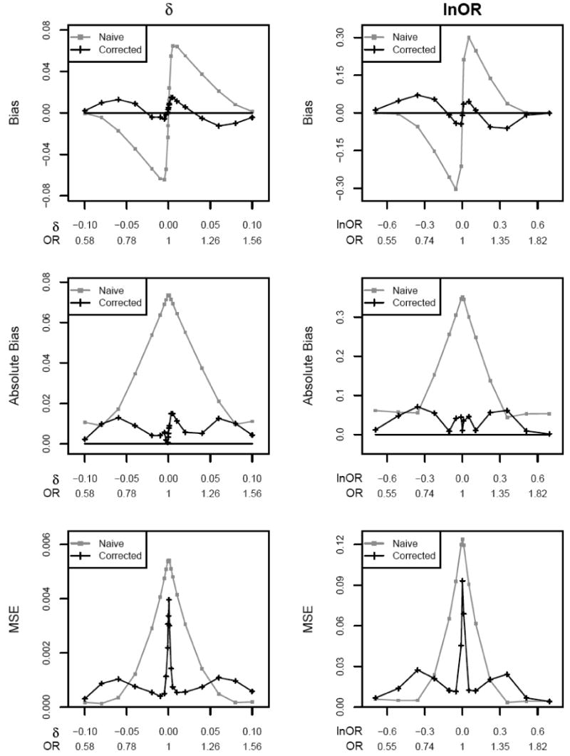
Bias, absolute bias, and mean square error (MSE) for allele frequency difference δ and logarithm of odds ratio lnOR with sample size N = 1000 and control allele frequency p = .3. Significance level α = 10^-6.

Table 1.

Proportional bias (%) of the uncorrected (naïve) and ascertainment-corrected MLEs of the allele frequency difference δ and odds ratio OR. Results are presented only for δ > 0.

p	N	power	δ	$\frac{{\widehat{\delta }}_{\mathit{\text{un}}}-\delta }{\delta }$	$$\frac{{\widehat{\delta }}_{\mathit{\text{as}}}-\delta }{\delta }$$	OR	$\frac{\stackrel{‵}{O}{R}_{\mathit{\text{un}}}-\mathit{\text{OR}}}{\mathit{\text{OR}}}$	$\frac{\stackrel{‵}{O}{R}_{\mathit{\text{as}}}-\mathit{\text{OR}}}{\mathit{\text{OR}}}$
		.01	.0376	101.9	-4.3	1.436	53.3	-1.8
		.10	.0541	47.9	-12.4	1.640	27.9	-5.7
	500	.30	.0665	26.2	-16.1	1.798	17.6	-7.2
		.50	.0752	16.2	-14.2	1.913	11.9	-6.5
		.80	.0898	6.0	-8.2	2.108	5.55	-1.7
.1
		.01	.0258	103.1	-7.0	1.295	31.2	-1.9
		.10	.0370	48.1	-15.7	1.429	19.2	-4.2
	1000	.30	.0453	26.5	-18.3	1.530	12.3	-7.1
		.50	.0512	16.0	-16.2	1.603	8.36	-6.3
		.80	.0609	6.1	-9.3	1.726	3.77	-4.1
		.01	.0576	103.0	-9.0	1.260	27.2	-2.1
		.10	.0806	48.3	-16.8	1.384	17.3	-5.3
	500	.30	.0972	26.3	-18.3	1.483	11.2	-6.3
		.50	.1086	16.2	-14.3	1.555	7.72	-5.8
		.80	.1270	6.1	-9.2	1.681	3.51	-3.6
.5
		.01	.0405	104.0	-13.1	1.176	18.5	-2.0
		.10	.0571	48.3	-18.6	1.258	11.8	-4.2
	1000	.30	.0690	26.4	-18.3	1.320	7.7	-4.9
		.50	.0772	16.2	-15.0	1.365	5.4	-4.5
		.80	.0903	6.1	-10.4	1.441	2.4	-3.1

un: uncorrected; as: ascertainment-corrected

p: disease allele frequency in controls; N: sample size (number of cases and of controls)

Assume testing at significance level α = 10^-6

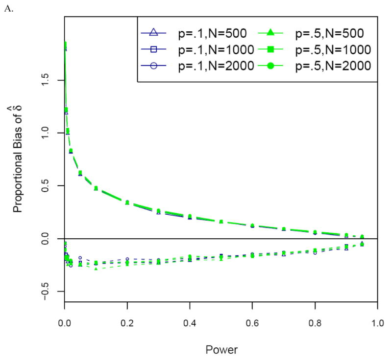
Figure 2.

Proportional bias versus power for the uncorrected (naïve) (solid lines) and corrected (dashed lines) estimators of the (A) allele frequency difference δ and (B) odds ratio OR. Significance level α = 10^-6. Results are presented only for δ > 0.

Given N = 1000 cases and N = 1000 controls, allele frequencies p = .1 and p+δ = .1258 (OR = 1.295), and testing at significance level of α = 10^-6 (resulting in power = .01), the expected value of the uncorrected estimator of δ is .0524 compared to the true value of .0258, a bias of .0266 and a proportional bias of 103%; similarly, the expected value of the uncorrected OR estimator is 1.699 compared to its true value of 1.295. In this case, a follow-up study designed to have 80% power at significance level α = .05 would include 310 cases and 310 controls, but would have actual power of only 30%.

We found that, for a fixed significance level α, the proportional bias in the uncorrected estimate of δ is solely a function of power, and is otherwise independent of sample size, allele frequency, or genetic model [Zöllner and Pritchard, 2007]. Consistent with intuition, proportional bias decreases as power increases (Figure 2A), since the conditioning event becomes increasingly likely. At significance level α = 10^-6, the uncorrected estimator of δ gives a proportional bias of ∼60% when power is .05 but is nearly unbiased when power is 95%. Interestingly, given fixed power, the proportional bias of the naïve estimator is consistently less when α = 10^-6 than when α = 10^-4.

We extended our analytical calculation to the uncorrected MLE of the odds ratio (Table 1, Figure 1), and observed the same general trend: substantial overestimation of the genetic effect given low to modest power to detect association and no bias given no association or sufficiently strong association. However, the proportional bias of the OR estimator, $\stackrel{‵}{O}{R}_{\mathit{\text{un}}}$, cannot be explained by power alone, but depends on sample size, allele frequency, and genetic model (Figure 2B). Interestingly, the proportional bias of the logarithm of the OR estimator, log $\stackrel{‵}{O}{R}_{\mathit{\text{un}}}$, is a function of power, and follows a very similar pattern as the uncorrected MLE of allele frequency δ.

Bias of the ascertainment-corrected MLE of δ and OR

When we correct for ascertainment, the absolute bias of the MLE is substantially reduced (Figure 1, Table 1), and correction actually results in underestimation unless the genetic effect size is small or power is very low. For example, given N = 1000 cases and N = 1000 controls, allele frequencies p = .1 and p+δ = .1258 (power = .01), and testing at significance level α = 10^-6, the proportional bias of the corrected MLE of δ is −7%, compared to +103% before correction. In this case, a follow-up study designed to have 80% power at significance level α = .05 would include 1350 cases and 1350 controls and have actual power 85%, whereas 1150 cases and 1150 controls actually would be sufficient to achieve 80% power. In the absence of association (δ=0), the corrected MLE is again nearly unbiased.

Reduction of the absolute bias is most pronounced when overestimation is most severe, and for fixed significance level α, bias reduction depends solely on study power. The relationship between power and proportional bias of the ascertainment-corrected MLE of δ is summarized in Figure 2A. Although the corrected MLE δˆ_as typically underestimates δ by 10-20% over the power range of .001-.95 given testing at significance level of α = 10^-6, the corrected MLE is considerably less biased than the uncorrected estimator unless power is high (typically > 60%). Even given high power, the magnitude of the bias of the ascertainment-corrected MLE δˆ_as is not much greater than that of the uncorrected MLE δˆ_un, and it is of opposite sign. Interestingly, when power greater than .1, the bias in the corrected MLE δˆ_as decreases almost linearly as power increases (Figure 2A).

The situation for the odds ratio is similar. With correction, the OR is typically underestimated by 5-10%, and this bias is in general smaller (although of opposite sign) than that for the uncorrected estimator for study powers ranging from .001 to .95 (Table 1, Figures 1 and 2B). Compared to the corrected MLE of δ whose proportional bias can be approximately summarized by power alone, the proportional bias for the corrected OR estimator does depends on sample size and allele frequency (Figure 2B), while the proportional bias of the logarithm of the corrected estimator depends essentially on power alone and displays a very similar pattern as that of the corrected estimator for δ (Figure 2A). Again, if we focus on the situations in which power < 60%, correction generally results in reduced absolute bias, and in many cases, absolute bias reduction is impressive. For example, given N = 1000 cases and N = 1000 controls, allele frequencies p = .1 and p+δ = .1258 (OR = 1.295), and testing at significance level α = 10^-6 (resulting in power = .01), the proportional bias of the corrected MLE of OR is −2%, compared to +31% before correction.

Standard errors and mean square errors (MSE) of the estimators

Table 2 summarizes the standard errors (SEs) for the MLEs of δ. We observed that the empirical SEs agree well with the asymptotic SEs for the corrected MLE, and both are two to six times greater than the SE of the uncorrected MLE which incorrectly ignores the fact of ascertainment. We also calculated the SE based on a random sample of the same sample size without ascertainment. All calculated SEs demonstrate that the genetic effect size estimates are quite variable in the settings described. The SEs of the corrected MLE are typically 1.5-2 times as large as those for an unascertained independent sample of the same size. This implies that while the ascertained sample is not as informative as a new random sample would be to estimate genetic effect size, the ascertained sample does provide 50-60% of the information in a new random sample, without the extra cost of collecting a new sample. We observed a very similar trend for SEs for the MLE of the odds ratio.

Table 2.

Standard errors (SEs) for the uncorrected (naïve) and ascertainment-corrected MLEs of the allele frequency difference δ and for MLE obtained from an unascertained random sample. Results are presented only for δ > 0.

p	N	power	OR	δ	SE
					δˆun	δˆas*	δˆas†	δˆrand
		.01	1.436	.0376	.0049	.0263	.0307	.0142
		.10	1.640	.0541	.0064	.0291	.0315	.0150
	500	.30	1.798	.0665	.0080	.0304	.0307	.0148
		.50	1.913	.0752	.0094	.0309	.0291	.0153
		.80	2.108	.0898	.0120	.0291	.0244	.0154
.1
		.01	1.295	.0258	.0032	.0179	.0216	.0099
		.10	1.429	.0370	.0043	.0200	.0212	.0103
	1000	.30	1.530	.0453	.0054	.0216	.0204	.0099
		.50	1.603	.0512	.0063	.0218	.0195	.0107
		.80	1.726	.0609	.0081	.0195	.0170	.0102
		.01	1.260	.0576	.0069	.0392	.0433	.0215
		.10	1.384	.0806	.0091	.0442	.0460	.0214
	500	.30	1.483	.0972	.0114	.0447	.0439	.0229
		.50	1.555	.1086	.0133	.0445	.0409	.0221
		.80	1.681	.1270	.0168	.0411	.0348	.0222
.5
		.01	1.176	.0405	.0049	.0280	.0319	.0159
		.10	1.258	.0571	.0065	.0310	.0320	.0154
	1000	.30	1.320	.0690	.0081	.0325	.0305	.0154
		.50	1.365	.0772	.0095	.0325	.0286	.0160
		.80	1.441	.0903	.0120	.0281	.0247	.0159

un: uncorrected; as: ascertainment-corrected; rand: random sample without ascertainment

^*: empirical;

^†: asymptotic

p: disease allele frequency in controls; N: sample size (number of cases and of controls)

Assume testing at significance level α = 10^-6

The mean squared error (MSE) provides a measure of estimator quality that takes into account both bias and variance. Figure 1 displays the MSE for the naïve and corrected MLEs of δ and lnOR. In general, the naïve estimator has larger MSE than the ascertainment-corrected estimator unless the genetic effect size is sufficiently large to result in high power to detect association. In that case, biases for the two estimators are similar but the variance of the corrected estimator is larger than that of the naïve estimator (Table 2).

II. Two-stage design

For both the allele frequency difference δ and the odds ratio OR, the naïve and ascertainment-corrected MLEs for optimal two-stage designs yield very similar results to those for the one-stage association designs described above (Figure 3A). This is hardly surprising, since for optimal two-stage designs, statistical power is very close to that of the corresponding one-stage design in which all markers are genotyped on all samples, and power (approximately) determines proportional bias for δ and lnOR. Even for non-optimal two-stage designs, this continues to be true, except that the proportional bias of both the uncorrected and corrected estimators tends to increase modestly as π_sample, the fraction of the sample genotyped in Stage 1, increases (Figure 3B).

Figure 3.

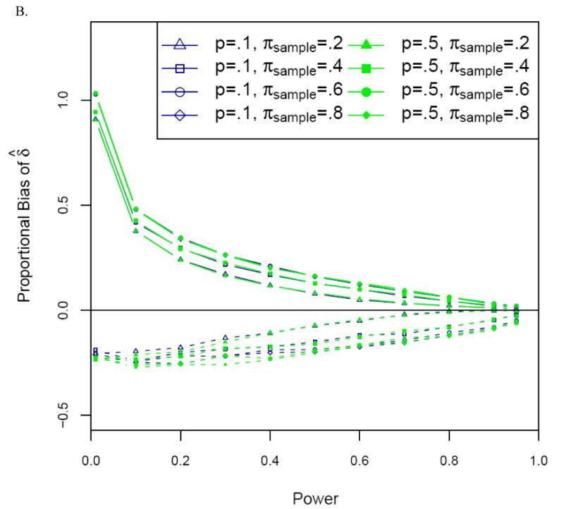
Proportional bias versus power for the uncorrected (naïve) (solid lines) and corrected (dashed lines) estimators of the allele frequency difference δ for (A) optimal and (B) non-optimal two-stage designs. Significance level α = 10^-6. Designs optimal for multiplicative disease model with disease prevalence .10, stage 2 to stage 1 genotype cost ratio 30. For non-optimal designs, π_marker = 1%, and samples of N=1000 cases and N=1000 controls. Results are presented only for δ > 0.

Discussion

In genetic association studies, the genetic effect size for associated markers tends to be overestimated as a consequence of winner's curse. This bias is due to the strong positive correlation between the association test statistic and the estimator of the genetic effect and the focus of investigators on markers that show statistically significant evidence of association. In this paper, we studied the bias of the naïve maximum likelihood estimators for the allele frequency difference and the odds ratio that ignore this ascertainment; these measures are routinely used to estimate the strength of the effect in genetic association studies. We demonstrated that the proportional bias in the estimators decreases as power increases. Interestingly, at fixed significance level, the proportional biases of the allele frequency difference and the logarithm of odds ratio are functions of power, and otherwise are essentially independent of allele frequency or sample size (see also [Zöllner and Pritchard, 2007]).

We proposed a maximum likelihood method to correct for this ascertainment bias. The ascertainment-corrected MLEs for both the allele frequency difference and the (log) odds ratio are generally less biased than the uncorrected estimators unless study power is moderate to high (>60%). Since large-scale genetic association studies of complex traits typically are underpowered owing to small genetic effect sizes, our method should generally provide a more accurate estimate of genetic effect size in the context of genome-wide association studies and large-scale candidate gene studies. In high power situations, bias for both the naïve and corrected methods are small, so that ascertainment correction again is reasonable. Proportional bias of the corrected and uncorrected estimators for both the allele frequency difference and the odds ratio does show modest dependence on significance level α. For example, when significance level α = 10^-4, biases for all estimators are somewhat increased compared to the case of α = 10^-6, and the advantage of ascertainment correction is increased slightly.

Zöllner and Pritchard [2007] used simulations to evaluate the impact of the winner's curse effect in genetic association studies and also proposed a maximum likelihood method to correct for it. Their method estimates the frequencies of all genotypes and corresponding penetrance parameters based on a known population prevalence of the disease under different inheritance models. In contrast, our method is simpler and focuses solely on the parameters of greatest interest: the allele frequency difference and odds ratio. This advantage of our method does require the assumption of Hardy-Weinberg Equilibrium for our case and control samples. Such an assumption is entirely reasonable given the modest locus effect sizes for complex traits, but would not be reasonable in the context of a Mendelian major locus.

Our corrected MLEs for the allele frequency difference and odds ratio generally underestimate the true genetic effects [Zöllner and Pritchard, 2007]. Using computer simulation, we note that the empirical distribution of our corrected MLEs can reasonably be described as a two-component mixture, with one component near zero and the other appearing more nearly normal. Figure 4 illustrates this for the ascertainment-corrected estimator of the allele frequency difference. As power increases, the distribution becomes more nearly normal, and the asymptotic unbiasedness of the MLE comes into play.

Figure 4.

Distribution of the ascertainment-corrected MLE of the allele frequency difference δ for different power levels. Results are presented only for δ > 0.

Based on 1000 simulation replicates of N=1000 cases and N=1000 controls, control allele frequency p = .5, and testing at significance level α = 10^-6.

We investigated the coverage of the asymptotic theory 95% confidence interval for the naïve and ascertainment-corrected MLEs for the allele frequency difference δ. The coverage of the ascertainment-corrected interval ranged from 82-100% for the cases we considered, reflecting the distribution and the bias of the ascertainment-corrected MLE, but still generally better than the coverage for the naïve estimator, which ranged from 0-92%.

Given the usual downward bias of our ascertainment-corrected estimators, one could consider an ad hoc bias correction. For the estimators of the allele frequency difference δ and the log odds ratio lnOR, the downward bias is 5-20% across the situations we considered (control allele frequency .1-.5, allele frequency difference δ=.018-.159 (OR 1.11-2.30), case and control sample sizes 250 to 2,000, and statistical significance 10^-4 to 10^-8), so that multiplying the resulting estimate by 1.05 – 1.10 would generally reduce absolute bias. However, such an approach is counterproductive when power is very low (<.005). The same criticism holds for taking a (weighted) average of the corrected and uncorrected estimators. More appealing might be to use an alternative estimation approach, and we currently are considering an empirical Bayes method [Carlin and Louis, 2000] that uses information from genome-wide association studies to help define a prior distribution for the genetic effect size.

Realistically, precise and unbiased estimation of genetic effect size will best be obtained by collecting a large sample specifically for this purpose, should resources be available to do so. However, given a sample in which an association is discovered, our ascertainment corrected approach provides more accurate estimation of allele frequency difference and odds ratio than the naïve approach, and permits better design of subsequent replication studies or studies focused on estimating the population effect of the identified variant(s). Standard errors for the ascertainment-corrected MLEs were substantially larger than those for the naïve estimator based on an independent random sample of the same size, correctly reflecting the information loss for estimation based on a sample used for association detection.

In summary, we have presented analytic calculations that quantify the impact of the winner's curse in large-scale genetic association studies, and confirm that in realistic situations, it can result in substantial overestimation of the true genetic effect as measured by the case-control allele frequency difference or the corresponding odds ratio. We propose a maximum likelihood estimator that corrects for the typical focus on statistically significant results, and demonstrate that this estimator results in reduced absolute bias compared to the naïve uncorrected estimator when study power is low or moderate (<60%), a range that is typical for most large-scale genetic association studies, and similar absolute bias when power is high. Our method does not require specification of a genetic model and is easy to implement. We extended these calculations to two-stage association studies, and found similar results to those for one-stage studies. We recommend the use of this ascertainment-corrected method for estimation of genetic effect size in large-scale genetic association studies.

Software that carries out this analysis for case-controls data is available at http://csg.sph.umich.edu/boehnke/winner.

Appendix

Calculate the observed information matrix I for one-stage study:

$$\begin{array}{l}I(p,\delta )=\left(\begin{array}{cc}a& b\\ b& d\end{array}\right),\text{where}\\ a=-\frac{m_0}{p^2}-\frac{2N-m_0}{{(1-p)}^2}-\frac{m_1}{{(p+\delta )}^2}-\frac{2N-m_1}{{(1-p-\delta )}^2}+\frac{A^2}{F^2}+\frac{B}{F}\\ b=-\frac{m_1}{{(p+\delta )}^2}-\frac{2N-m_1}{{(1-p-\delta )}^2}+\frac{AD}{F^2}+\frac{C}{F}\\ d=-\frac{m_1}{{(p+\delta )}^2}-\frac{2N-m_1}{{(1-p-\delta )}^2}+\frac{D^2}{F^2}+\frac{E}{F}\end{array}$$

where A, B, C, D, E and F are calculated as follows:

$$\begin{array}{l}A=\sum _{(x_0,x_1)\in I}\left\{\left(\frac{x_0}{p}-\frac{2N-x_0}{1-p}+\frac{x_1}{p+\delta }-\frac{2N-x_1}{1-p-\delta }\right)P(x_0,x_1)\right\}\\ B=\sum _{(x_0,x_1)\in I}\left\{\left(\frac{x_0}{p^2}+\frac{2N-x_0}{{(1-p)}^2}+\frac{x_1}{{(p+\delta )}^2}+\frac{2N-x_1}{{(1-p-\delta )}^2}-{\left(\frac{x_0}{p}-\frac{2N-x_0}{1-p}+\frac{x_1}{p+\delta }-\frac{2N-x_1}{1-p-\delta }\right)}^2\right)P(x_0,x_1)\right\}\\ C=\sum _{(x_0,x_1)\in I}\left\{\left(\frac{x_1}{{(p+\delta )}^2}+\frac{2N-x_1}{{(1-p-\delta )}^2}-\left(\frac{x_0}{p}-\frac{2N-x_0}{1-p}\right)\times \left(\frac{x_0}{p}-\frac{2N-x_0}{1-p}+\frac{x_1}{p+\delta }-\frac{2N-x_1}{1-p-\delta }\right)\right)P(x_0,x_1)\right\}\\ D=\sum _{(x_0,x_1)\in I}\left\{\left(\frac{x_1}{p+\delta }-\frac{2N-x_1}{1-p-\delta }\right)P(x_0,x_1)\right\}\\ E=\sum _{(x_0,x_1)\in I}\left\{\left(\frac{x_1}{{(p+\delta )}^2}+\frac{2N-x_1}{{(1-p-\delta )}^2}-{\left(\frac{x_1}{p+\delta }-\frac{2N-x_1}{1-p-\delta }\right)}^2\right)P(x_0,x_1)\right\}\\ F=\sum _{(x_0,x_1)\in I}P(x_0,x_1)\end{array}$$

where I = {(x₀, x₁) : X (x₀, x₁) > x_α} and P(x₀, x₁) is calculated by formula (2) in the paper.

Our calculation for the asymptotic SE for p and δ was based on the observed information matrix evaluated at pˆ_as, δˆ_as.

References

- Allison DB, Fernandez JR, Heo M, Zhu S, Etzel C, Beasley TM, Amos CI. Bias in estimates of quantitative-trait-locus effect in genome scans: demonstration of the phenomenon and a method-of-moments procedure for reducing bias. Am J Hum Genet. 2002;70:575–585. doi: 10.1086/339273. [DOI] [PMC free article] [PubMed] [Google Scholar]
- Bazerman MH, Samuelson WF. I won the auction but don't want the prize. J Conflict Resolut. 1983;27:618–634. [Google Scholar]
- Carlin BP, Louis TA. Bayes and empirical Bayes methods for data analysis. 2nd. CRC Press; Boca Raton, FL: 2000. [Google Scholar]
- Garner C. Upward bias in odds ratio estimates from genome-wide association studies. Genet Epidemiol. 2007;31:288–295. doi: 10.1002/gepi.20209. [DOI] [PubMed] [Google Scholar]
- Ghosh A, Zou F, Wright FA. Estimating odds ratios in genome scans: an approximate conditional likelihood approach. Am J Hum Genet. 2008;82:1064–1074. doi: 10.1016/j.ajhg.2008.03.002. [DOI] [PMC free article] [PubMed] [Google Scholar]
- Göring HHH, Terwilliger JD, Blangero J. Large upward bias in estimation of locus-specific effects from genomewide scans. Am J Hum Genet. 2001;69:1357–1369. doi: 10.1086/324471. [DOI] [PMC free article] [PubMed] [Google Scholar]
- Ioannidis JP, Ntzani EE, Trikalinos TA, Contopoulos-Ioannidis DG. Replication validity of genetic association studies. Nat Genet. 2001;29:306–309. doi: 10.1038/ng749. [DOI] [PubMed] [Google Scholar]
- Lohmueller KE, Pearce CL, Pike M, Lander ES, Hirschhorn JN. Meta-analysis of genetic association studies supports a contribution of common variants to susceptibility to common disease. Nat Genet. 2003;33:177–182. doi: 10.1038/ng1071. [DOI] [PubMed] [Google Scholar]
- Nelder JA, Mead R. A simplex method for function minimization. Computer J. 1965;7:308–313. [Google Scholar]
- Rao CR. Linear statistical inference and its applications. New York: John Wiley; 1965. [Google Scholar]
- Satagopan JM, Verbel DA, Venkatraman ES, Offit KE, Begg CB. Two-stage design for gene-disease association studies. Biometrics. 2002;58:163–170. doi: 10.1111/j.0006-341x.2002.00163.x. [DOI] [PMC free article] [PubMed] [Google Scholar]
- Siegmund D. Upward bias in estimation of genetic effects. Am J Hum Genet. 2002;71:1183–1188. doi: 10.1086/343819. [DOI] [PMC free article] [PubMed] [Google Scholar]
- Skol AD, Scott LJ, Abecasis GR, Boehnke M. Joint analysis is more efficient than replication-based analysis for two-stage genome-wide association studies. Nat Genet. 2006;38:209–213. doi: 10.1038/ng1706. [DOI] [PubMed] [Google Scholar]
- Skol AD, Scott LJ, Abecasis GR, Boehnke M. Optimal designs for two-stage genome-wide association studies. Genet Epidemiol. 2007;31:776–788. doi: 10.1002/gepi.20240. [DOI] [PubMed] [Google Scholar]
- Sun L, Bull SB. Reduction of selection bias in genome-wide studies by resampling. Genet Epidemiol. 2005;28:352–367. doi: 10.1002/gepi.20068. [DOI] [PubMed] [Google Scholar]
- Wu LY, Sun L, Bull SB. Locus-specific heritability estimation via bootstrap in linkage scans for quantitative trait loci. Hum Hered. 2006;62:84–96. doi: 10.1159/000096096. [DOI] [PubMed] [Google Scholar]
- Yu K, Chatterjee N, Wheeler W, Li Q, Wang S, Rothman N, Wacholder S. Flexible design for following up positive findings. Am J Hum Genet. 2007;81:540–551. doi: 10.1086/520678. [DOI] [PMC free article] [PubMed] [Google Scholar]
- Zhong H, Prentice RL. Bias-reduced estimators and confidence intervals for odds ratios in genome-wide association studies. Biostatistics. 2008 doi: 10.1093/biostatistics/kxn001. in press. [DOI] [PMC free article] [PubMed] [Google Scholar]
- Zöllner S, Pritchard JK. Overcoming the winner's curse: estimating penetrance parameters from case-control data. Am J Hum Genet. 2007;80:605–615. doi: 10.1086/512821. [DOI] [PMC free article] [PubMed] [Google Scholar]