

Abstract
Identifying and validating novel phenotypes from images inputting online is a major challenge against high-content RNA interference (RNAi) screening. Newly discovered phenotypes should be visually distinct from existing ones and make biological sense. An online phenotype discovery method featuring adaptive phenotype modeling and iterative cluster merging using improved gap statistics is proposed. Clustering results based on compactness criteria and Gaussian mixture models (GMM) for existing phenotypes iteratively modify each other by multiple hypothesis test and model optimization based on minimum classification error (MCE). The method works well on discovering new phenotypes adaptively when applied to both of synthetic datasets and RNAi high content screen (HCS) images with ground truth labels.
Keywords: online phenotype discovery, RNA interference, high content screen, gap statistics, minimum classification error
1. Introduction
Cells have the ability to dramatically alter their shape in response to specific environmental cues, models on signaling networks regulating cell shape are needed to design effective therapeutics for treatment of cancer, neuron-generative diseases, and pathogen infection [1], and Drosophila genome-wide high-content RNA interference (RNAi) screen (HCS, high-content screen) is employed to construct such models. RNAi HCS visualizes various morphological phenotypes caused by knocking down different genes [2, 3], and we must identify and quantify such phenotypes to assign a unique role for each gene in the regulation of cell shape. Expert ground truth labeling of phenotypes performed well in small scale screens [4] but it is infeasible to manually analyze HCS data. Several methods have been proposed to automatically classify cells into previously well-defined phenotypes [5], and the definition of such phenotypes involves some well trained biologists going over the whole dataset to gain a crude assessment of phenotype variance. However such supervised analysis is difficult to cover all the meaningful phenotypes in screens where millions of images are acquired and we have to automatically identify novel phenotypes online using crude assessment on existing phenotypes.
Ideally, online phenotype discovery methods should be designed to utilize dataset from existing phenotypes and solve four challenging tasks, i.e. 1)restoring those existing and biologically meaningful phenotypes, 2) differentiating novel phenotypes from existing ones, 3) clarifying novel phenotypes from each other and 4) updating the database and models for existing phenotypes along with online image input. Task 3) and 4) make online phenotype discovery distinct from simply identifying outliers, because it is necessary to differentiate multiple novel phenotypes from each other, rather than generally labeling them as “outliers”, what’s more, once a novel phenotypes is detected online, it is no longer “outliers” and should be modeled and involved into the database of existing phenotypes. Such transformation from “novel” to “known” makes it critical to update the phenotype models online while the continuously increase of sample size makes such model updating difficult.
In this paper, we present an online phenotype discovery method consisting of two key components: adaptive phenotype modeling and iterative cluster merging. After constructing cell data base (with thousands of cells) for important phenotypes through expert ground truth labeling, we build Gaussian Mixture Model (GMM) for each existing phenotype following [6], such model depicts the properties of each existing phenotype and make it possible to judge the effect and confidence level for restoring an existing phenotype or defining a novel one. When a new image (with tens of cells in each image) comes, GMM of each existing phenotype is sampled and combined with the new image one by one. For each combined dataset, we estimate cluster number using gap statistics [7]. Gap statistic is an established framework which can make significant estimation on cluster number and is compatible to various clustering method, here it is used to predict how many groups of cells in the new image can be considered as different from the existing phenotype. By combine a same new image with the existing phenotypes one by one rather than together, we circumvent the difficulties in aforementioned task 1) and focus on differentiating novel phenotypes from known ones in this stage. Considering the distinct properties between different phenotypes, we modified the strategy of taking reference dataset for gap statistics, that is, null distributions for existing phenotypes and the new image are estimated separately to make better use of the expert ground truth involved in defining existing phenotypes and avoid generating sparse sample dataset. The modified strategy helps improve the overall performance on restoring biologically meaningful phenotypes. After cluster number estimation, we perform clustering on the combined dataset. Due to the necessity of frequently running the clustering, a method using compactness criterion, Partitioning Around Medoids (PAM) [8], is selected for its efficiency and effectiveness. Part of cells from new image are merged by existing phenotype according to clustering results and cells remaining in new image are iteratively combined with other existing phenotypes, such iterative merging and updating steps restore the existing phenotypes one by one from the new image. Cell clusters never merged by any existing phenotypes are considered as candidates of new phenotype, and the partitions given by clustering results are indications for clarifying novel phenotypes from each other (aforementioned task 3).
We construct a bridge between clustering results given by PAM and GMM estimated using Bayesian parameter inference. The merging operation is validated using multiple hypothesis tests where the merging decision made by clustering can be rejected by p-values (with Bonferroni correction considering multiple existing phenotypes) generated from GMM and the influence from the outlier of model sampling are repressed. This step confirms the confidence of restoring existing phenotypes. On the other hand, the continuous adding of new images extends our knowledge on the existing phenotypes and urges an efficient updating of phenotype models along with the online image input (aforementioned task 4). After all the existing phenotypes merged their counterpart in one new image, the GMM of all phenotypes are optimized using minimum classification error (MCE) model as proposed in [6], MCE method updates GMM according to the classification result from a small sample set and avoids heavy computational burden. Here partition from PAM is used to define classification errors. Thus clustering results and GMM iteratively modify each other, the inconsistency between clustering and GMM is reduced iteratively and finally more reliable phenotype models are acquired.
Figure 1 illustrates the tasks of online phenotype discovery, the general workflow of our method, with key steps for fitting in the online scenario highlighted in red bounding boxes.
Figure 1. Tasks of online phenotype discovery for high-content RNAi screens.

Our method is tested on one synthetic image dataset defined according to real cell images as well as two published dataset related to high content RNAi screen. Experimental results show that the proposed method is robust and efficient for online phenotype discovery in not only the context of the RNAi screen described in this work, but to diverse image-based screens.
In Section 2 of this paper, each step of online phenotype discovery method are discussed in detail, and section 3 presents experiment results on phenotype merging and discovery. Discussion and conclusion remarks are given in Section 4.
2. Methods
2.1 Problem Formulation
Suppose we have identified K0 non-overlapping cellular phenotypes, the i-th cell in the m-th existing phenotype is denoted by vector , with each cell described by P morphological features. Then, let denote the set of all cells in the m-th phenotype, with um indicating the number of cells in Sm. Thus, the set of all the available cells S is defined as:
| (1) |
and the total number of existing cells is . When a new image E comes, its i-th cell is denoted by , and , where ν is the number of cells in E. We usually have tens of cells in each E, while thousands cells exist in each Sm, i.e. ν<<um<u.
Given E, we must determine number of new phenotypes Knew, based on, K0, S and E. The issue of v<<u makes it unfeasible to involve every single cell in S into cluster discovery, because the large scale of S could bias cluster analysis towards clusters with larger sample number, and also add computation burden. On the other hand, “new cluster” identified only according to E is vulnerable to outliers. Thus an efficient method of utilizing S is necessary.
2.2 Outline of the Approach
We propose to discover new phenotypes online through iterative cluster merging. Dataset of each existing phenotype Sm is first fit to a GMM and this model is sampled to form a dataset S’m with feasible sample number. Each S ’m, m∈{1,2…K0 } is combined with the new image E one by one to detect possible new phenotypes. The method runs as listed below.
Modeling each existing phenotype. A GMM is fit to each existing phenotype.
-
Sampling existing phenotype and combining sample set with new image. We sample from the GMM of one existing phenotype, say Sm, m ∈{1, 2…K0 }, get the sample set S’m, and combine it with new image E to get a combined set F, i.e.
(2) We empirically select sample number of S’m as ν to 5ν.
-
Estimating the cluster number in F using improved gap statistics [7].
-
(3a)
Sampling reference datasets separately for S’m and E, using GMM as reference distribution for samples from S’m and uniform distribution for samples from E, the support of two reference distributions are defined by binding box along the values of S’m and E, respectively.
-
(3c)
Combining the above two reference dataset and estimating the cluster number in F based on the combined reference dataset using gap statistics [7].
-
(3a)
Defining clusters on F . F is clustered into the estimated cluster number in step 3, and the clustering approach of PAM [8] is utilized.
-
Merging cells into existing phenotypes.
-
(5a)
Defining the candidates for merging. Such candidates include samples from E while assigned to a same cluster with at least 95% samples from S’m.
-
(5b)
Validate the merging operation through a statistical test with Bonferroni correction.
-
(5c)
When the operation of merging one cell into phenotype Sm is validated, adding it to Sm while removing it from E.
-
(5a)
Going back to step 2, sampling from the GMM of another existing phenotype and starting a new merging loop with modified E (previously merged cells have been removed), looping until all existing phenotypes have been combined with E.
-
Updating phenotype models.
-
(7a)
Defining clusters left in E as new phenotypes and estimate GMM for them.
-
(7b)
Summarizing decision rules from the conditional distribution models given by GMM for each phenotype, classifying each cell in the original E using these rules.
-
(7c)
Figuring out the “classification errors”, i.e. the inconsistency between classification result in (7b) and clustering result after (6).
-
(7d)
Optimizing all GMM using MCE method and awaiting new image.
-
(7a)
Through modeling and re-sampling, S becomes more flexible and re-useable, and we can cover the properties of each phenotypes more completely. The information from existing phenotypes is combined with new image one by one in step 3 to 5. Thus in each single loop, the task of estimating cluster number is simplified to identifying difference between new image E and only one existing phenotype. After each Sm merges its counterpart in E, clusters left in E are identified as new phenotypes.
2.3 Cluster Modeling and Sampling
Given the dataset of existing cells S, we model each phenotype Sm using a GMM:
| (3) |
where N denotes Gaussian distribution. We denote the number of Gaussian terms for phenotype Sm as Qm and define parameters for Sm as . Each, μm,t has P entries as μm,t =[μm,t [1], μm,t [2],…μm,t [P ]]; and the covariance matrix Σm,t are set to be diagonal initially as Σm,t =diag (σm,t [1],σm,t [2]…σm,t [P ]).
We use Expectation-maximization (EM) algorithm to estimate {πm, μm, Σm } from Sm. In the initialization of EM algorithm, Qm is set four, and Sm is first partitioned into Qm clusters using fuzzy C-means clustering method, and then initial parameters are estimated using the standard vector quantization method. For each class, the number of Gaussian terms Qm is reduced to the minimum possible using minimum description length (MDL) technique, following [6]. For each single cell e, the conditional distribution of each phenotype Sm is defined as
| (4) |
We obtain random samples from the GMM to form set S’m having i.i.d Sm, S’m, and S’m is combined with new image E to form F. When estimating cluster number in F using gap statistics, GMM is used as reference distribution for S’m.
2.4 Estimating Cluster Numbers using Improved Gap Statistics with GMM as Reference Distribution
To solve the problem of estimating cluster numbers, many existing methods focus on the within cluster dispersion Wk, resulting from clustering datasets (e.g. F) into k clusters, C1, C2,…Ck with Cr denoting the indices of samples in clusters r and fi,j denotes the value of j-th feature measured from i-th data point. Based on , we have . Wk tends to decrease monotonically as the number of clusters k increases, but from some k on, such decrease flattens markedly. Statistical folklore has it that error measure based on Wk should have an “elbow” at the desirable cluster number, thus different criterions based on Wk are defined.
Gap statistics [7] method utilizes the output of any clustering algorithm under different k, compares the change of Wk to the dispersion expected under a reference null distribution, the gap between the logarithms of these two dispersions are employed to detect cluster number. Gap statistics can detect homogenous non-clustered data against the alternative of clustered data [9]. This ability is critical when all cells in new image E belong to the same phenotype.
To estimate cluster number in F (defined in equation (2)), we first select a number K which is larger than the expected cluster number, e.g. in our case K=10. For each k=1, 2…K, F is divided into k clusters and gives a series of Wk. Then we generate B reference datasets from F, cluster them into k clusters and obtain W*kb, b =1, 2,…B, k =1, 2,…K. We use PAM [8] for clustering. Considering the mean dispersion across B (B=15 in our case) reference datasets, and their standard deviation , an item is taken into consideration for a better control about the rejection of null model [7], and estimated cluster number K ’ is obtained as below:
| (5) |
The reference distribution is a null model of data structure. In [7], reference sets are sampled uniformly either from the range of observed values for each feature, or the range of a box aligned with the principle components of data. However it is encouraged to estimate reference distribution from existing samples rather than simply using uniform distribution. Because the binding box of the whole dataset will always include some “blank” area without any samples, and the existing cluster definition can help us focus on where the data really lies, and avoid generating a sparse reference dataset which ignores the property of original dataset. Here, S’m we sampled S’m from GMM of each existing phenotype. Therefore, it makes sense to use this GMM as the reference distribution for S’m.
The problem now is to generate reference dataset from GMM, because S’m is combined with new image E to form the dataset F, and the model of E is unavailable. We have to deal with S’m and E separately because the distribution of E is unavailable. We propose to solve this problem by generating reference dataset from S’m (GMM as reference distribution) and E (uniform distribution as reference distribution) separately and combine two sets together, i.e. substituting Supp(F) = Supp (E∪S’m) with
| (6) |
Figure 2 illustrates the strategies used for taking reference dataset. Similar as the original gap statistics method, our method can define the support of reference distribution using different “bounding boxes”. In the following experiments, all the supports are defined as the binding box aligned to the feature axes.
Figure 2. Take reference data set separately for existing clusters (red circles) and new dataset (blue circles).

GMM is an accurate model for S’m, and using GMM as reference distribution can avoid the risk of splitting one existing phenotype. Biological properties of existing phenotypes are retained, and novel phenotypes in new images become more outstanding under uniform reference distribution. Our modification on taking reference distribution not only restores the ability of characterizing the shape of datasets (different bounding boxes), but also improve it by excluding the blank area of the dataset (handling S’m and E separately).
2.5 Cluster Definition and Merging
We use Partitioning Around Medoids (PAM; also known as K-medoids) [8] to do clustering on combined set F. PAM provides better flexibility and robustness of choosing suitable dissimilarity measurements for different applications [10] and more efficient compared to clustering methods like Fuzzy C-means, especially in our merging loops where the clustering would be carried frequently.
After clustering, we get a non-overlapping partition on combined dataset F, we denote this partition as , where the cluster number K’ is determined through gap statistics, and we adjust the cluster labels to make sure that F1 includes the largest ratio of samples from existing phenotype S’m. Merging operation is done according to this partition. In our merging loops, datasets S’m,m∈{1, 2,…K0} are combined with E one by one, and in each merging loop, the overlapped part of S’m and E (if any) are located in F1 and is deleted from E and included as part of existing cluster:
| (7) |
after all merging loops, clusters left in E are defined as new phenotypes.
The above merging strategy is based on theoretical case of F1⊇S’m, but in reality, when we consider random sample set S’m from GMM of a existing phenotype, it is possible that some samples are randomly far from the centre of existing phenotype and thus assigned into different clusters with their majority counterparts in S’m. To prevent the influence from such outliers, two strategies are utilized to validate our merging operation.
Merging operations only happen when some cells in E are assigned into F1, and meanwhile F1 contains more than 95% of samples in S’m. And such samples in E are considered candidates for merging operation.
Given the existing phenotype Sm and each merging candidate ej, we carry out multiple hypothesis test with Bonferroni correction to validate the merging operation. A p-value is calculated based on the conditional distribution model Sm(ej) given in equation (4). This p-value indicates the possibility of obtaining a value at least as extreme as (if not more) this candidate under this GMM for S’m. The corrected p-value for ej is defined as its p-value with respect to Sm divided by the number of existing phenotypes K0,. If the corrected p-value is lower than 0.05/K0, the merging operation is rejected and we keep ej in E, or else ej is merged into Sm and deleted from E.
Figure 3 illustrates how the cluster merging loops work on a synthetic dataset. After all the merging loops, we define the number of identified novel phenotypes as Knew. We estimate a GMM for each newly identified phenotype and further optimize all the existing GMM based on minimum classification error.
Figure 3. Illustration of merging loops on a synthetic data set.
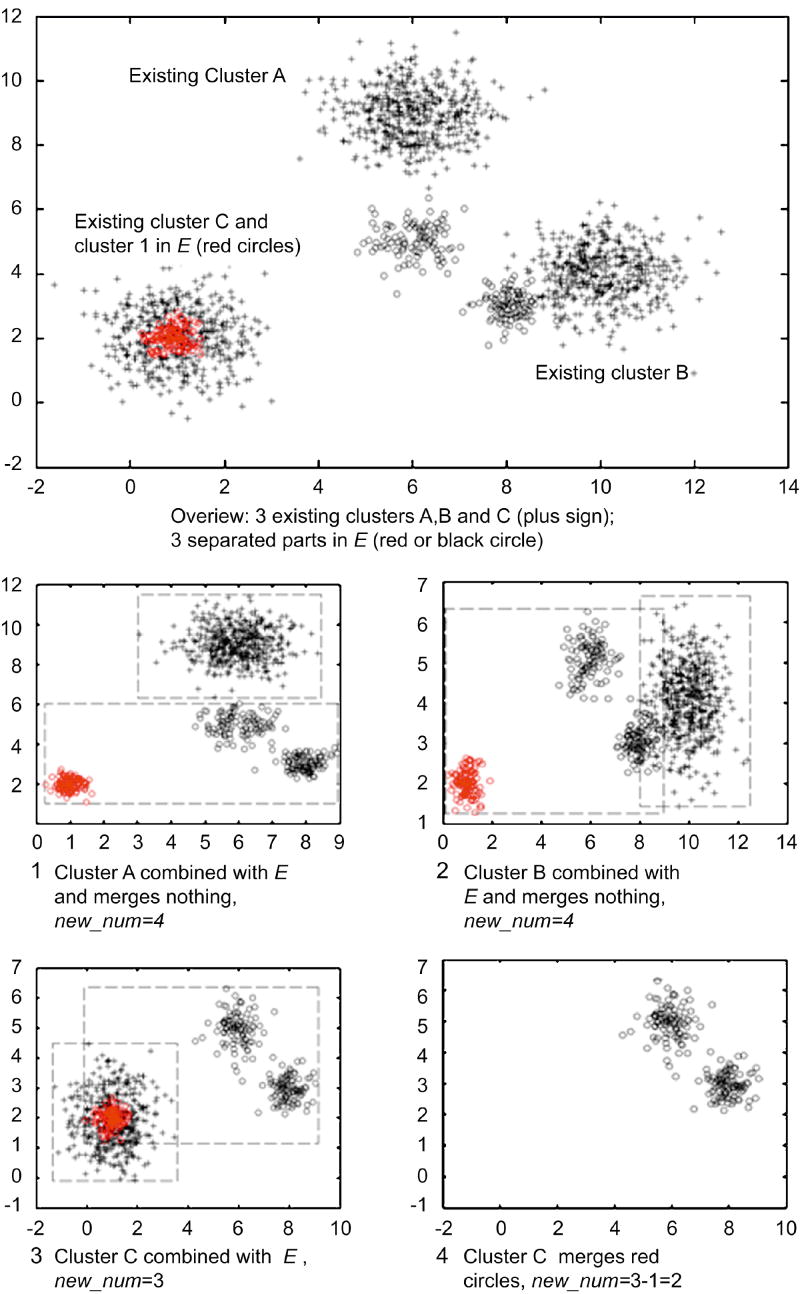
The largest subplot shows the overview of a synthetic dataset, and four smaller subplots labeled as 1-4 shows three merging loop (1-3) and the final result of carrying out iterative cluster merging on this dataset
2.6 Online Optimization of GMM based on Minimum Classification Error
In this step, we optimize all the phenotype models so that they can restore the clustering result in future loop. Now that we have identified Knew novel phenotypes from image E, and using PAM clustering method, all the ν cells in original E are assigned into K0+ Knew clusters, denoted as C1, C2,…Ck0+Knew, with Cm denoting the indices of samples in clusters m according to the result from PAM clustering. On the other hand, a GMM has been estimated for each phenotype and a series of classifiers can be built regarding to the conditional distribution shown in equation (4), and a series of classes C̃1, C̃2,…C̃K0+Knew are thus defined, with C̃m denoting the indices of samples assigned to the m-th class. The ultimate target of phenotype modeling is to make C̃m=Cm,m =1,2…K0+Knew, i.e. the GMM should restore the operation made by the clustering (merging of cells or definition of new phenotypes), and make sure that similar cells in future images can be assigned in a same cluster. Such consistency between clustering and classification result is critical when a new cluster has just been identified, and the number of cells used to build the GMM are not so large. For such phenotypes, we must adjust the GMM to include new members indicated by clustering.
Thus, after obtaining K0+Knew clusters from E, we continue to refine the conditional distribution models by adjusting the parameters , similar to [6] this is done by minimizing a penalty function that is related to the classification error, while in our case, the classification error is defined as the inconsistency between clustering result Cm and classification result C̃m given by GMM.
Given a vector e representing a single cell from the original new image E, we consider a set of class conditional likelihood function given by
| (8) |
We define the parameter set related to Sm(e) as , And the entire parameter set of the classifier is . For ei,i=1,2…ν (each cell in the image E) and C̃m (the set of cell indices assigned to class m) the decision rule based on GMM is given by
| (9) |
Define the following class misclassification measure
| (10) |
Where η is a positive number. Hence, dm (e) >0 implies misclassification and dm (e) ≤0 means correct decision. Next, we define the following empirical penalty function of the parameter set Λ based on the classification result for all v cells in image E
| (11) |
where
| (12) |
| (13) |
with γ being a constant. Notice that the logic function is defined using the clustering result Cm, thus this method add penalty to the inconsistency between C̃m and Cm, and thus update GMM to make C̃m consistent with Cm.
In order to maintain the original constraints in the GMM, we apply the following transformations on the parameters: (i)πm,t → π̃m,t, where πm,t = exp {π̃m,t} / Σi exp {π̃m,t}; (ii) μm,t [p ]→μ̃m,t [p ]=μm,t [p ]/σm,t [p ] and (iii) σm,t [p ] → σ̃m,t [p ]=logσm,t [p ], where p= 1, 2…P.
To minimize L (Λ) with respect to Λ, we use the stochastic gradient algorithm. Starting from the nth cell in image E, the mixture weights are updated according to
| (14) |
with
| (15) |
where
| (16) |
The elements in the mean vectors are updated according to
| (17) |
with
| (18) |
where [x]p denotes the p-th entry of a vector x.
And the elements in the covariance matrices are updated following
| (19) |
with
| (20) |
In our experiments, we choose the following parameters: η =1,γ =0.4 , and the step sizes e1 (0)=0.01, e1 (n)=e2 (n)=e1 (0)n0.8 and e3 (n)=0.2 e1 (n).
3. Experiments and results
3.1 Synthetic dataset
3.1.1 Dataset Description
After going over fluorescent microscopy cell images generated for Drosophila genome wide RNAi screen (Bakal et al, unpublished), we picked up seven types of cells (RGB colour image) and simulated them using seven types of polygons in 8-bit gray level images (256 level gray scale with intensity 0 indicating black and 255 for pure white). The information of these cells and polygons are shown in Figure 4.
Figure 4. Information of seven types of polygons used as synthetic dataset.

The key geometry and gray level parameters of each polygon were sampled from random variables defined according to the information from real cells. For instance, gray level filled into an ellipse was sampled from uniform distribution in the range of [0, 50], while the rectangles were filled with gray levels sampled uniformly from the range of [120, 180]. Each polygon was described using six features, including mean and standard deviation of gray levels, and geometry features like length of longest axis, length of shortest axis, perimeter and area of the polygons.
We generated 2000 polygons from each of seven types to serve as training dataset, i.e. the set of existing phenotypes, and we also had another 2000 polygons from each type to form the test dataset, i.e. cells in a series of synthetic images used to carry out experiments. In each experiment, we started from a certain set of existing phenotypes and built GMM from training samples. On the other hand, we iteratively chose two of seven polygon types and selected 100 polygons apiece out of the testing dataset to form a synthetic test image, altogether 70 images can be formed for one experiment. Using the model estimated from training set, we can identify existing and novel type of polygons from these synthetic images, and observe the performance of our method under different number of novel phenotypes and order of image input.
3.1.2 Performance under different sets of existing phenotypes
Figure 5 shows the general performance of our method under different sets of existing phenotypes. Figure 5 left shows the performance of the method with improved gap statistics and MCE model optimization, and these results are compared with the performance of the method with improved gap statistics but no model optimization, which are listed in Figure 5 right.
Figure 5. Performance of two online phenotype discovery methods on the synthetic dataset.

left) The method with improved gap statistics and MCE model optimization; right) The method with improved gap statistics but no model updating. The number along X axis shows the number of phenotypes used as existing phenotypes. All the accuracy values for each phenotype are averaged across different composition of existing phenotypes (when number of existing phenotypes varies from 1 to 6, the number of possible compositions are 7, 21, 35, 35, 21 and 7, respectively) and 50 different order of image input for each composition.
We changed the number and composition of existing phenotypes, (composition means which types are chosen as “existing”), and for each set of existing phenotypes, we shuffled the order of image input 50 times. Whatever set of existing phenotypes we used, the synthetic images always contained all seven phenotypes and we can always define accuracy for each polygon type as “the proportion of test samples restored into its original cluster”. If one phenotype is used as existing phenotype in one experiment, the accuracy on this phenotype is defined as the proportion of testing cells (in this phenotype) merged into the that existing cluster; while if the phenotype is novel, the accuracy of this phenotype equals the proportion of testing cells left along in a separate cluster after all the merging loops. Thus, we can average the accuracy across all different order of image input and composition of existing phenotypes to report the general performance of our method under different experiment conditions.
We can see from Figure 5 that our method have consistent performance for different polygon types under different conditions, with all the accuracy values over 85%, and the best performance comes when the number of existing phenotypes are 3 and 4. What’s more, the method with GMM optimization based on MCE continuously outperforms the method without model optimization step. The model optimization procedure dramatically improves the performance on most polygon types when the number of existing phenotypes is lower than 3. This is consistent with our expectation of adding the model updating steps: modifying the models for novel phenotypes according to the clustering result so that it can characterize the new phenotype better with relatively low number of training samples. When the number of existing phenotype is 6, both method suffered from false negative (especially for rectangle and trapezoid phenotypes) as novel samples were merged into existing phenotypes, and this indicates the importance of cluster validation and the necessity of more refined multiple hypothesis tests.
3.1.3 Modifications on gap statistics and model updating improve the performance
Specifically, we pick up two sets of experiments both with six existing phenotypes, and compare the performance of three online phenotype discovery methods. One series of experiments are carried out with ellipses serve as novel phenotype, and the other series have 16-point star as novel phenotype. Both types of experiments have 70 test images with 200 polygons each, the order of image input are shuffled 50 times and the average accuracy for each polygon type is shown in Figure 6.
Figure 6. Performance of three online phenotype discovery methods on two specific experiments on synthetic dataset.

left) Average performance across 50 experiments with ellipses serve as novel phenotype; right) Average performance across 50 experiments with 16-point stars serve as novel phenotype. The accuracy on an existing phenotype is defined as the ratio of testing cells in this phenotype and merged to its original phenotypes; and the accuracy for a novel phenotype is calculated as the proportion of test cells in this phenotype, while left alone in a separate cluster after all the merging loops.
All of the three involved methods are based on iterative cluster merging, but one directly uses gap statistics to estimate the cluster numbers, one uses improved gap statistics with reference dataset sampled separately, and the other one is the method proposed here, with improved gap statistics as well as phenotype model optimization using MCE. We can see from Figure 6 that the method here outperforms the other two in at least five of six phenotypes.
The method using original gap statistics suffers from the complicated composition of existing phenotype, especially when distinct phenotypes of rectangles and 16-point stars are both used as existing phenotypes (Figure 6 left). Taking reference dataset separately from each existing phenotype dramatically improves the performance, because the reference dataset focus on where the samples really lies, and thus each reference dataset is less sparse and more representative than taken from a single distribution with support defined by the whole dataset.
In both type of experiments, the accuracy on the novel phenotype is improved by the involvement of model optimization based on MCE. After a novel phenotype is identified, the GMM is estimated based on a small amount of samples, and following samples in this phenotype are prone to be mistakenly merged into existing phenotypes. With the phenotype models continuously updated according to each new image, such false merging is effectively avoided, and the accuracy related to novel phenotypes are improved.
3.2 Performance validation on published genetic screening dataset aiming at defining local signalling networks regulating cell morphology
3.2.1 Dataset Description
We download quantified data related to [1] from http://arep.med.harvard.edu/QMS and use it to validate our method’s ability of restoring biological meaningful clusters. In this dataset, the morphological change of 12601 cell segments from 249 different treatment conditions (TCs) are described by twelve morphological indicators. A quantitative morphological signature (QMS) is defined for each TC based on the morphological change it causes. All TCs are clustered based on their QMS, and seven out of 41 resulted clusters are highlighted in [7]. We selected altogether 6782 cell segments from six of these biological meaningful clusters and use their quantified morphology indicators to carry out our experiments. The information of those six clusters is summarized in Table 1.
The work in [1] represents the recent attempt of using fluorescent microscopy images based genetic screen to define local network regulating cell morphology. Gene over-expression and double-stranded RNA (dsRNA) induced RNAi are utilized individually or in combination to form altogether 249 TCs. A QMS is defined for each TC according to the observed morphological change on cultured Drosophila BG-2 Cells. Through cell culturing, stochastic labeling and segmentation, altogether 12601 individual cells are obtained for analysis..
Three level of quantification are employed to generate the QMS for each TC: from individual cell image to 145 morphological features for each cell; from 145 features to a group of twelve morphological indicators for each cell (constructing twelve neural networks (NN) based on twelve group of training cells with typical morphological changes and measuring the similarity between each cell and each of the training sets); and from morphological features of each cell to QMS for each TC (a normalized Z-score across all the cells for a same TC). Seven scores are used to form final QMS vector for each TC.
3.2.2 Restoring biological meaningful clusters
In this case we try to validate the ability of restoring biological meaningful “pheno-clusters” for our method. Six phenol-clusters highlighted in [1], namely Cluster 6, 8, 18, 33, 1 and 27 are used. Quantified morphological indicators for 2,800 cell segments are divided into a flow of image input consisting of 28 synthetic images with 100 cells in each image. Two series of experiments with different sets of existing pheno-clusters are carried out and the performances of three online phenotype discovery methods are compared. Both kinds of experiments are repeated 100 times with different order of inputting test images. Figure 7 shows the result of these experiments.
Figure 7. Performance comparisons among three methods on restoring biological meaningful cluster from published high throughput screen data.

left) Average performance across 100 experiments with cluster 1 and 27 serve as novel phenotype; right) Average performance across 100 experiments with cluster 23, 1 and 27 serve as novel phenotype.
We get similar trends as in the synthetic datasets. The method proposed in this paper outperforms the other two methods in at least four of six phenol-clusters, and also improve the accuracy on novel phenotypes. Specifically, adding cluster 33 into the group of existing phenotypes helps improve the results. Cluster 18 is the largest phenol-cluster in the dataset, featuring large, flat cells typically with extensive lamellipodia, and cluster 27 includes three TCs featuring cells displaying an aberrant number of long protrusions [1], by adding cluster 33 (featuring cells subject to dsRNA TCs targeting at Rho1 family) to existing phenotypes, we can identify cells with spiky and polarity structure better, thus reduce the possibility of merging cells in cluster 27 into cluster 18.
This case shows our method’s ability of restoring biological meaningful clusters/phenotypes in the online scenario, and supplies the confidence for applying our method when trying to extend genetic screen in [1] to genome wide scale.
3.3 Identifying novel phenotype from high-content RNAi genome-wide screening
3.3.1 Dataset Description
We utilized the fluorescence images mentioned in [5]. A genome wide RNAi screen was carried out to implicate genes involved in Rac (a subfamily of the Rho family GTPases) signaling using Drosophila Kc167 cell line. The corresponding cellular phenotypes were analyzed for changes, and the authors present a framework of analysis with the core step of classifying the cells into three pre-defined phenotypes, namely normal, ruffle and spiky.
Image Acquisition and Segmentation
All the fluorescent images are obtained following the protocol in [5], among three channels in the original color images, cytological profiling was based on analyzing cell shapes in the gray level image of actin channel. A two-step segmentation method is involved in cell segmentation. It includes nuclei segmentation on DNA channel, and cell body segmentation on the combined images of Actin, Tubulin and DNA channels [11, 12, 13]. In the nuclei segmentation, the nuclei are first detected by a background correction based adaptive threshold method and the gradient vector field. Then the clustered nuclei are segmented using the marker watershed algorithm. Segmentation results of nuclei are used as the ‘seed’ images for marker watershed based cell body segmentation. To accurately delineate the boundaries of cell bodies, an automated feedback system is used to reduce the over-segmentation of cells following [12]. Detailed shape and boundary information of nuclei and cell bodies is obtained after the segmentation procedure.
Morphological Feature Extraction and Feature Selection
To capture the geometric and appearance properties, we extract 211 cellular morphology features belonging to five categories following [5], including 85 wavelet features, 10 Zernike moments features, 48 Haralick features, 14 geometric region property features, and 54 phenotype shape descriptor features. To describe the dataset more informatively, an unsupervised feature selection method is adopted. It is based on iterative feature elimination using k nearest neighbor (kNN) features, following [14]. We use correlation coefficients as the similarity measure for each pair of features, iteratively pick up the feature having biggest correlation coefficient with its kNN features, discard these k neighbor features and update parameter k until k is reduced to 1. A set of 15 features is finally selected.
Training and testing dataset
We use the three phenotype defined in [5] as the existing phenotypes. To assure the reliability of models for existing phenotypes, we pick up an extended training dataset from the combination of the original 1 000-cell-patch database in [5] and the cells processed from the whole genome wide screen. Using the EM algorithm, a GMM with two Gaussian items are fit to normal phenotypes, while ruffle and spiky phenotype end up with four Gaussian items, respectively. Another 1 000 cells are selected as testing dataset. The information of our training and testing dataset is listed in Table 2.
3.3.2 Box and whisker plot showing the performance on restoring existing phenotypes
Using the 1000 testing cells from three phenotypes, we form a flow of ten synthetic images; each image contains 100 cells from two of three phenotypes. Using our method of online phenotype discovery with improved gap statistics and model optimization based on MCE, we try to merge those testing cells into their original phenotypes using the GMM estimated in previous step. The order of image input is shuffled 100 times and the accuracy for each phenotype is calculated. Across the 100 repeated experiments, the average accuracy for normal phenotype is 91.49%, with standard deviation of 1.11%; some cells in ruffle phenotype are not merged due to the various texture property caused by actin accumulation, and the average accuracy still reach 87.10%, with standard deviation of 1.44%; and the spiky phenotype has an average accuracy of 90.87% and standard deviation of 1.35%.
We rank the accuracy from each experiment, and illustrate the performance using box and whisker plot. The accuracy for each phenotype in each experiment is sorted in descending order and plotted along the Y-axis, the two horizontal edges of boxes indicate upper and lower quartile of accuracy values while the red line in the middle shows the median value. The whiskers and lines extending from the end of boxes show the extent of the rest data, and red crosses (+) are outliers with accuracy values beyond 1.5 times of inter quartile range. The box plots for all three phenotypes are shown in Figure 8. With all the inter quartile range smaller than 5%, we can confirm the robustness of our method against different order of image input.
Figure 8. Performance on restoring existing phenotypes from testing dataset.

3.3.3 Discovering novel phenotypes from the genome wide RNAi screen
Finally we combine our method with the whole dataset of genome wide RNAi screens. Starting from the three existing phenotypes, we identified another three novel phenotypes, and the information about these phenotypes is shown in Table 3. These phenotypes are different from the original ones in level of actin accumulation (uniform, punctuate or highly accumulated), distribution of actin (along the boundary or across cell body), size and stage of polar formation, etc. The biological mechanism behind these phenotypes remains to be explored, but by doubling the number of morphological phenotypes, our method does show its ability to supply a better insight into the high content RNAi screen, and based on the method in [5] as well as our discovery, a more versatile scoring system can be built to better reveal the detailed role of genes involved in the screen.
At present stage, all functions are developed in Matlab 7.0 and run in PC with Intel® Core™ 2 T7200 2.00GHz CPU and 2.00GB of RAM. Starting from three existing phenotypes, the average running time for the method based on improved gap statistics and model optimization using MCE is 2.2 seconds on a group of 100 segmented cells, 13.2 seconds on a group of 600 cells and 25.4 seconds on a group of 1000 cells. When we change the PAM clustering method into fuzzy C-means method from the fuzzy logic toolbox of Matlab, the average running time on a group of 100 cells is larger than 30 seconds, which is intractable for online application. On the other hand, k-means method is as efficiency as PAM method, our method using PAM outperforms k-means based method on the accuracy of restoring existing phenotypes by 2-5%. Considering the fact that cell number in each image is seldom over 300 in the reported high content screen, our method recruit proper technologies to solve all the major challenge against online phenotype discovery and the present framework is efficiency and robust for online application.
4. Discussion and Conclusions
Identifying novel morphological phenotypes online is a major challenge in specific high-throughput image-based screens. Manual phenotype labeling of high-throughput image-based data is a laborious and inordinately time-consuming process, while available automatic identification methods usually classify cells into a limited set of predefined phenotypes which have been determined through biased means and won’t be updated according to the online image input. As millions of images are now generated during the course of a comprehensive genome-scale screen new methods are needed to effectively identify novel phenotypes in such massive databases. Here we report the development of an online phenotype discovery method which models existing phenotypes, compares cells in new images with existing phenotype models through cluster analysis, assigns some new cells to existing phenotypes, and finally identifies and validates novel phenotypes online.
Instead of hanging with single Gaussian model, we use Gaussian mixture model to describe each biologically meaningful cluster. Theoretically GMM can approximate closely any continuous density function for a sufficient number of mixtures and appropriate model parameters [15]. Gap statistics plays a key role in cluster analysis and merging. Using GMM as the reference distribution for the existing phenotypes in gap statistics, we can cover the complete properties of phenotypes more efficiently. Furthermore, we iteratively combine the new image with the sample set from each existing phenotypes and update the content of new image. Thus the task in each loop is simplified to compare part of new image with only one existing phenotype.
Originally, clustering based on compactness criteria and methods based on GMM are of different types. We set a bridge between them through two ways, one is multiple hypothesis test used for cluster validation and another is model optimization based on MCE methods. The former step validates the merging operation based on the GMM to avoid the influence of outliers while the latter one modifies the GMM to get more robust results.
For analysis of high content screen data, many researchers choose to summarize the information of single cells or objects to supply a normalized signature for higher level concepts (e.g. treatment conditions, genes, complexes, etc). Thus it is critical to identify different phenotypes related to a same treatment condition. When applied to the analysis of high content screens, our method can be involved in identifying multiple phenotypes related to single well, help the definition of refined phenotype signature and supply more detailed insight into related questions. Under the frame of iterative cluster merging, our future goals are to build more reliable phenotype models, construct complete pipelines of cluster analysis with validation procedures and finally obtain more reliable definition of phenotypes.
Acknowledgments
We would like to thank colleagues of Perrimon Lab in the Department of Genetics at Harvard Medical School, for their excellent collaboration. The authors would also like to thank research members of The Methodist Hospital Research Institute, Radiology Department. The research is funded by The Methodist Hospital Research Institute (Stephen T.C. Wong).
Footnotes
Publisher's Disclaimer: This is a PDF file of an unedited manuscript that has been accepted for publication. As a service to our customers we are providing this early version of the manuscript. The manuscript will undergo copyediting, typesetting, and review of the resulting proof before it is published in its final citable form. Please note that during the production process errors may be discovered which could affect the content, and all legal disclaimers that apply to the journal pertain.
References
- 1.Bakal C, Aach J, Church G, Perrimon N. Quantitative morphological signatures define local signaling networks regulating cell morphology. Science. 2007;316:1753–1756. doi: 10.1126/science.1140324. [DOI] [PubMed] [Google Scholar]
- 2.Friedman A, Perrimon N. A functional genomic RNAi screen for novel regulators of RTK/ERK signaling. Nature. 2006;444:230–234. doi: 10.1038/nature05280. [DOI] [PubMed] [Google Scholar]
- 3.Friedman A, Perrimon N. Genetic screening for signal transduction in the era of network biology. Cell. 2007;128:225–231. doi: 10.1016/j.cell.2007.01.007. [DOI] [PubMed] [Google Scholar]
- 4.Kiger AA, Baum B, Jones S, Jones MR, Coulson A, Echeverri C, Perrimon N. A functional genomic analysis of cell morphology using RNA interference. Journal of Biology. 2003;2(27):271–285. doi: 10.1186/1475-4924-2-27. [DOI] [PMC free article] [PubMed] [Google Scholar]
- 5.Wang J, Zhou X, Bradley PL, Perrimon N, Wong STC. Phenotype recognition for high-content RNAi genome-wide screening. Journal of Molecular Screening. 2008;13:29–39. doi: 10.1177/1087057107311223. [DOI] [PubMed] [Google Scholar]
- 6.Zhou X, Wang X. Optimisation of Gaussian mixture model for satellite image classification. IEE Proc-Vision, Image and Signal Process. 2006;153(3):349–356. [Google Scholar]
- 7.Tibshirani R, Walther G, Hastie T. Estimating the number of clusters in a dataset via the gap statistic. J Royal Stat Soc B. 2001;32(2):411–423. [Google Scholar]
- 8.Kaufman L, Rousseeuw P. Finding groups in Data: An introduction to Cluster Analysis. Wiley; New York: 1990. [Google Scholar]
- 9.Yan M, Ye K. Determining the Number of Clusters Using the Weighted Gap Statistics. Biometrics. 2007;63:1031–1037. doi: 10.1111/j.1541-0420.2007.00784.x. [DOI] [PubMed] [Google Scholar]
- 10.Thalamuth A, Mukhopadhyay I, Zheng X, Tseng G. Evaluation and comparison of gene clustering methods in microarray analysis. Bioinformatics. 2006;22(19):2405–2412. doi: 10.1093/bioinformatics/btl406. [DOI] [PubMed] [Google Scholar]
- 11.Zhou X, Liu KY, Bradley PL, Perrimon N, Wong STC. Towards automated cellular image segmentation for RNAi genome-wide screening. Lecture Notes in Computer Science; MICCAI 2005; pp. 885–892. [DOI] [PubMed] [Google Scholar]
- 12.Yan P, Zhou X, Shah M, Wong STC. Automatic Segmentation of RNAi Fluorescent Cellular Images with Interaction Model. IEEE Trans on Info Tech in Biomedicine. 2008;12(1):109–117. doi: 10.1109/TITB.2007.898006. [DOI] [PMC free article] [PubMed] [Google Scholar]
- 13.Li FH, Zhou X, Wong STC. An automated feedback system with the hybrid model of scoring and classification for solving over-segmentation problems in RNAi high content screening. Journal of Microscopy. 2007;226(2):121–132. doi: 10.1111/j.1365-2818.2007.01762.x. [DOI] [PubMed] [Google Scholar]
- 14.Mitra P, Murthy CA, Pal S. Unsupervised Feature Selection Using Feature Similarity. IEEE Trans PAMI. 2002;24(3):301–312. [Google Scholar]
- 15.Zhao Y, Zhuang X, Ting S. Gaussian mixture density modeling of non-Gaussian source for autoregressive process. IEEE Trans Signal Processing. 1995;43(4):894–903. doi: 10.1109/83.535841. [DOI] [PubMed] [Google Scholar]