Abstract
We present a novel method called RosettaHoles for visual and quantitative assessment of underpacking in the protein core. RosettaHoles generates a set of spherical cavity balls that fill the empty volume between atoms in the protein interior. For visualization, the cavity balls are aggregated into contiguous overlapping clusters and small cavities are discarded, leaving an uncluttered representation of the unfilled regions of space in a structure. For quantitative analysis, the cavity ball data are used to estimate the probability of observing a given cavity in a high-resolution crystal structure. RosettaHoles provides excellent discrimination between real and computationally generated structures, is predictive of incorrect regions in models, identifies problematic structures in the Protein Data Bank, and promises to be a useful validation tool for newly solved experimental structures.
Keywords: protein structure/folding, structure, crystallography, computational analysis of protein structure, protein structure prediction, hydrophobic interactions, protein structures—new underpacking, validation, visualization
Introduction
Tight packing of side chains in protein cores is crucial to protein folding and stability. Protein cores are packed as tightly as corresponding crystals, and mutations that disrupt a protein core strongly reduce the free energy of folding.1–3 The near absence of voids in protein cores is in part a reflection of the large free energy cost of forming a protein-sized cavity in water, which increases steeply with the total volume of the structure, including voids.
Much work has been done in the assessment of protein core packing. The most widely used packing-related metric is the Leonard-Jones (LJ) interaction energy, which favors nonbonded atom pairs that are close together but not overlapping. The LJ energy, along with the majority of other commonly used force-field terms and scoring methods, is pairwise additive: each pair of atoms in a structure is evaluated, and the results are summed. However, the void volume and cavity contribution to the solvation free energy cannot be accurately expressed as a sum of atom pairs. Cavity area and volume obey the inclusion–exclusion rule: total space filled is that filled by single atoms, minus two-body intersections, plus three body intersections, minus four body intersections, and so on, and cannot be accurately captured by pair-additive functions.
Multibody methods that directly measure cavities are typically based on a space-filling representation in which each atom is modeled as a hard sphere with radius equal to the van der Waals (VDW) radius of the atom. Setting the radius of the sphere to the physically reasonable VDW radius is problematic in that all empty space within the protein is usually contiguous with the outside of the protein. To produce explicit cavities, existing methods inflate the VDW radii, usually by the radius of a water molecule (1.4 Å), filling most interstitial space and cutting off remaining cavities from outside space. Several methods exist to characterize the explicit cavities in the inflated representation, including an approximate slicing method4 and the exact Alpha Shapes method.5,6 Unfortunately, the inflated atom representation washes out those geometric features of a protein that are smaller than 2.8 Å. For example, after inflating VDW radii, a long, narrow crack would disappear. In a close-packed lattice of carbon atoms, voids larger then 2.8 Å do not appear until the spacing is increased by 40%. We have found in practice that features finer-grained than 2.8 Å are important in assessing packing quality.
To avoid the loss of detail inevitable in an inflated VDW model of voids and packing, we have developed a new method, RosettaHoles, that generates a set of void-filling balls that cover the interstitial space in an uninflated VDW model. In regions surrounding cavities, we measure the contact surface area for 30 probe radii ranging from 0.1 to 3.0 Å in size, yielding a wealth of data about packing of atoms around each cavity. We then employ a support vector machine (SVM)7 trained to distinguish high-resolution crystal structures from poorly packed theoretical model. The resulting score is an estimate of the probability that a given atomic arrangement is like those in high-resolution crystal structures. This score has been used extensively in our laboratory for assessment of predictions and designs produced with Rosetta8 and has proven very effective in distinguishing well-packed, high-resolution crystal structures from poorly packed computationally generated models. When applied to experimentally determined models, we find that the RosettaHoles score of structures in the Protein Data Bank (PDB) depends heavily on experimental method and X-ray resolution and that many structures with poor scores are known to be problematic in some way. We believe RosettaHoles will be useful in validating newly determined experimental structures as well as theoretical models of natural and designed proteins.
Results
Summary of method and testing
As described in detail in Methods section, RosettaHoles starts by finding the largest spherical hole adjacent to each buried atom in the VDW structure and then pruning away balls that are accessible to a water-sized probe. The remaining cavity balls are the basis for both visualization and quantitative analysis of core packing. For visualization, the spherical holes are clustered into contiguous cavities, and small clusters are pruned away. See Figures 1 and 2 for an illustration and the methods section for details. Quantitative analysis is based on the contact surface area with respect to various sized probes, computed for atomic shells surrounding empty spaces in the protein. These surface area statistics are aggregated via a Support Vector Machine (SVM) into the RosettaHoles score, which estimates the probability that a structural region came from a high resolution crystal structure, and root-mean-squared distance (RMSDpred), in a local region of a model to the corresponding crystal structure. Training and testing were performed on three data sets of computational protein structure predictions and designs from Rosetta.
Figure 1.
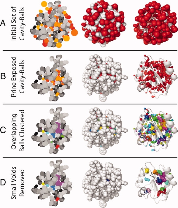
Overview of cavity computation and visualization. (A) All of the spheres computed based on vertices of the approximate Apollonius diagram. (B) Balls remaining after those exposed to the surface are pruned away. (C) Balls clustered into contiguous cavities with an arbitrary color for each cavity. (D) Final clusters remaining after small cavities have been pruned away. In the flat slices on the left, colors are shaded by depth for clarity.
Figure 2.
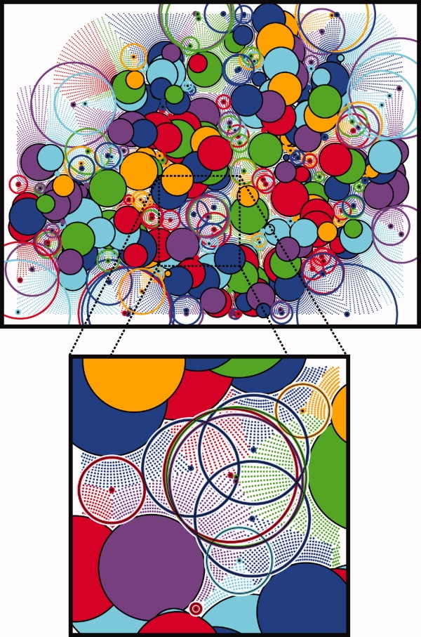
Calculation of cavity balls. Pictured is the result of a 2D implementation of our cavity finding process performed on a slice through the center of heat shock operon repressor HrcA (arbitrarily selected example). Shaded circles represent atoms and the surrounding like-colored dots are closer to that atom than any other. The furthest dot for each atom, which approximates the vertex of the ideal Apollonius diagram, is marked as a larger like-colored dot with a black center. Centered on these dots are the largest empty circles that fit around each vertex and do not intersect any atom. These circles are the 2D analog of the cavity filling balls in our method. Slices of atoms closer to the camera overlap those further from the camera and coloration is arbitrary.
We show that RosettaHoles applies generally to computationally generated models by analysis of fullatom structure predictions submitted by all groups in the 7th Critical Assessment of Structure Prediction (CASP7). To assess the usefulness of our method on experimentally solved structures, we analyze the packing quality of all structures in the PDB.
Illustration
Figure 3 illustrates explicit cavity visualization and RosettaHoles scores from SVM training. An experimentally determined structure is shown in panels A, B, C, D, along with a corresponding structure prediction in panels E, F, G, and H. Panels A and E show the unadorned crystal and predicted structures, respectively. Panels B and F show the cavities superimposed on the structures, colored by contiguous cavities. The balls clearly indicate the cavities in the computationally generated model. Panels C, D, G, and H show the RosettaHoles score on a color scale from red (bad packing = 0) to green (good packing = 1). A slice through the colored VDW structures is shown in panels D and H. Surface atoms tend to be colored blue as they have neutral packing scores. The poor packing in the computationally generated model shows up clearly in both the explicit cavity representation 3(B,F) and in coloration by RosettaHoles score (compare red regions in D/H).
Figure 3.
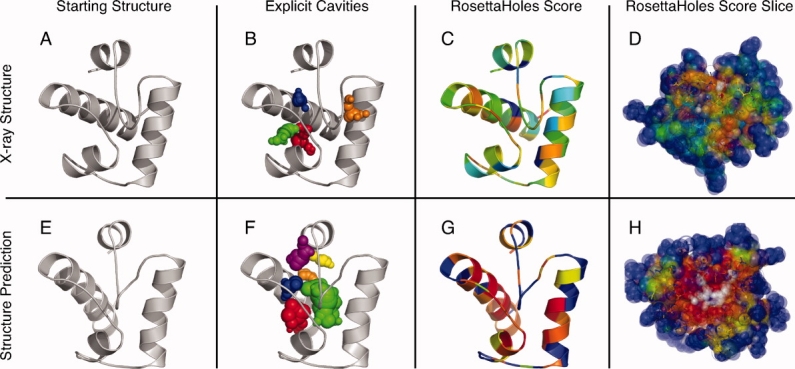
Visualization of cavities. The top panels A, B, C, and D show a crystal structure of CASP6 target 199, heat shock operon repressor HrcA, and the bottom panels E, F, G, and H show a computational structure prediction for this protein. The leftmost panels A and E show the unadorned structure. Panels B and F show the structure with cavity clusters represented explicitly in arbitrary colors to distinguish cavities. The structures in panels C, D, G, and H are colored by the numerical packing score described in the text. The color scale ranges from green to blue to red, with the worst packed regions in red.
Comparison of packing metric in experimental and computed structures
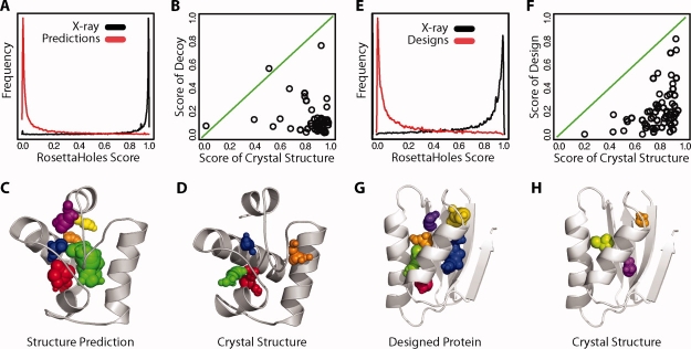
The RosettaHoles scores shown by coloration in Figure 3(D,H) show a qualitative difference between the crystal structure and the flawed computational model. Figure 4 shows a quantitative comparison of RosettaHoles between crystal and computationally generated structures for a broad range of proteins. Figure 4(A) shows a density plot of RosettaHoles scores for the void-centered regions in data set 1 (see methods), with structure predictions in red and corresponding crystal structures proteins in black. There is a clear separation, receiver operating characteristic (ROC) of 0.943, between atomic shells from crystal versus computationally generated models. Figure 4(B) shows the RosettaHoles scores of whole structures, the median of the scores over all regional scores for a structure. In almost all cases, the computationally generated model scores significantly worse than the crystal structure. These aggregate RosettaHoles scores have an ROC score of 0.972. Figure 4(C,D) shows an example structure pair from the data set, a computationally generated model in 4C and the corresponding crystal structure in 4C. The difference in packing quality is visually clear. A similar separation in RosettaHoles score is observed between a set of fixed backbone protein designs and corresponding crystal structures, as shown in Figure 4(E,F). Atomic shells from designed proteins can be differentiated from similar regions from crystal structures fairly reliably with an ROC score of 0.934 [Fig. 4(E)] and aggregate packing scores for whole structures separate designs from crystal structures with an ROC score of 0.980 [Fig. 4(F)]. As in the structure prediction data, almost all computed models score worse than the experimentally determined structure. Figure 4(G,H) shows an example design and crystal structure pair.
Figure 4.
Packing quality of protein structure predictions and designs. (A) Distribution of RosettaHoles scores for cavities in predicted and crystal structures (ROC 0.943). In red are the estimated RosettaHoles scores of structure predictions for 42 proteins and in black is the distribution of scores for the set of corresponding crystal structures. (B) RosettaHoles whole-structure score for 42 structure predictions plotted against the score of the corresponding crystal structure. (C) Structure prediction for CASP target 199. (D) Crystal structure for target 199. (E) Distribution of RosettaHoles scores for individual cavities (ROC 0.934). In red are the RosettaHoles scores of fixed backbone redesigns of 62 proteins and in black is the distribution of scores for the set of corresponding crystal structures. (F) RosettaHoles whole-structure score for the 62 designs plotted against the score of the corresponding crystal structure. (G) Fixed backbone design of protein 1cc8. (F) Crystal structure for 1cc8.
Correlation of packing metric with local structure quality
In the discrimination tests, we observed that the RosettaHoles scores for local regions of a structural model are a powerful predictor of how much those region deviate from the corresponding region of a crystal structure. Following up on this observation, we tested the correlation between local RMSD to crystal structure and RMSDpred, the packing based predictor of local RMSD, for 12 large (200–400 residue) CASP7 targets. Predicted RMSDpred was computed exactly as the RosettaHoles scores (see methods) except that SVM regression was used rather than SVM discrimination. RMSDs to crystal structure were measured over the same local regions used in generating the RMSDpred scores. For each of the 12 proteins, local regions for comparative models were sorted into bins based on RMSDpred, and the median local RMSD for each bin was computed. Figure 5 shows the result for each of the 12 structures; the estimated RMSDpred bin is plotted on the x axis, and the median real RMSD for the bin on the y axis. The area of each plotted point is proportional to the number of local regions that scored in that bin. In the majority of cases, the median RMSD for each bin is correlated with RMSDpred, showing that packing information is predictive of local structure RMSD.
Figure 5.
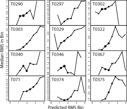
Correlation of local packing score with local RMSD. Predicted versus actual RMSD is shown for 12 large (200–400 residue) CASP7 targets. Predicted RMSD was computed exactly as the RosettaHoles scores except that SVM regression was used rather than SVM discrimination. RMSDs to crystal structure were measured over the same 7-Å radius balls of atoms used to compute the estimated RMSD. The atom balls were binned on predicted local RMSD, shown on the x-axis, and the median true RMSD is plotted on the y-axis. The area of each plotted point is proportional to the number of local regions which scored in that bin.
Packing analysis on CASP7 models
Although we developed RosettaHoles for the analysis of structure predictions and designs generated with Rosetta, it detects similar packing flaws in computationally generated models submitted by other groups in CASP7. For each CASP7 target with a crystal structure available for reference, we computed packing scores for submitted models from all groups. Because it is impossible to fairly assess packing in models that do not include all heavy atoms, all models missing more than 5% of heavy atoms were discarded. Table I shows the percentile rank of the crystal structure among all the computational models for each target. For most targets, the crystal structure ranked better than all submitted models. In all but four cases, the crystal structure is in the top 3%, and in all but one case, the crystal structure is in the top 10%. All four of these cases are due to a low packing score for the crystal structure rather than an abundance of well-packed models (Supplementary Fig. S1).
Table I.
Packing Score Percentile of Crystal Structure Among CASP7 Targets
| Target | Percentile | Target | Percentile | Target | Percentile |
|---|---|---|---|---|---|
| t283 | 97.5 | t320 | 100.0 | t346 | 97.5 |
| t285 | 97.0 | t321 | 99.2 | t347 | 100.0 |
| t286 | 100.0 | t322 | 100.0 | t348 | 95.2 |
| t288 | 100.0 | t323 | 100.0 | t359 | 93.7 |
| t290 | 98.4 | t324 | 100.0 | t362 | 100.0 |
| t292 | 97.6 | t325 | 100.0 | t364 | 97.0 |
| t297 | 100.0 | t328 | 99.2 | t367 | 100.0 |
| t298 | 99.1 | t329 | 100.0 | t369 | 100.0 |
| t300 | 88.0 | t330 | 100.0 | t371 | 100.0 |
| t301 | 100.0 | t331 | 100.0 | t372 | 98.4 |
| t304 | 97.9 | t332 | 100.0 | t374 | 100.0 |
| t306 | 99.1 | t333 | 100.0 | t375 | 100.0 |
| t307 | 97.6 | t334 | 100.0 | t376 | 100.0 |
| t308 | 98.8 | t338 | 100.0 | t378 | 100.0 |
| t309 | 93.5 | t339 | 100.0 | t379 | 100.0 |
| t312 | 96.9 | t340 | 97.7 | t382 | 99.3 |
| t313 | 97.5 | t342 | 100.0 | t383 | 99.3 |
| t315 | 100.0 | t345 | 100.0 | t385 | 100.0 |
| t316 | 100.0 | t346 | 97.5 | t386 | 94.1 |
| t319 | 91.0 |
The percentile rank of the crystal structure (correct answer) among all structure predictions submitted in CASP7.
Packing analysis of structures in the PDB
We performed a systematic analysis of packing quality for all PDB structures larger than 50 residues in size and containing less than 10% nucleic acid (circa April 2008). For the analysis of PDB structures, only heavy atoms were considered because most structures contain few if any hydrogen atoms but all heavy atoms are typically present. All heteroatoms other than hydrogen and water were included. The RosettaHoles score was found to be highly correlated with experimental method and crystallographic resolution. Figure 6 shows density plots of the packing score for various X-ray resolution bins as well as for NMR structures and CASP7 models. Very high-resolution crystal structures (sub-1.0 Å) have systematically better packing scores than all other structures; a 95th percentile structure between 1.0 and 2.0 Å in resolution would be merely average for 1.0 Å or better resolution. Similarly, a 95th percentile NMR structure would be average among 1–2 Å crystal structures. The computationally generated fullatom models submitted to CASP7 are systematically worse than all experimentally solved structures.
Figure 6.
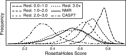
Packing score distributions of predicted and experimental structures. Density plots of the packing score for different X-ray resolution bins as well as for NMR structures and CASP7 models submitted by all groups. Very high-resolution crystal structures (sub-1.0 Å) have systematically better packing scores than all other structures; a 95 percentile structure between 1.0 and 2.0 Å resolution would be merely average for 1.0 Å or better resolution. Similarly, a 95th percentile NMR structure would be average among 1 to 2 Å crystal structures. The computationally generated fullatom models submitted to CASP7 are much worse than experimentally solved structures.
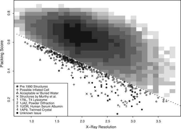
The RosettaHoles score is plotted versus resolution for 38,061 crystal structures in Figure 7. For clarity, the majority of the structures in the plot are shown in a 2D histogram, with only points below the dotted line shown explicitly. The plotted points, especially the very lowest ones, have unusually bad packing scores for their resolution. Many of these structures were published before 1990, suggesting an increase in structure quality since that time. For some outliers, especially among the sub-2.0 Å resolution structures, the inclusion of low B-factor buried waters often raises the packing score above the plotted diagonal line. Eight of the outliers, (PDB codes 2A01, 1BEF, 1RID, 1Y8E, 1BGX, 1G44, 2QID, 1G40) are from the Murthy group.9
Figure 7.
Assessment of PDB structures using RosettaHoles score. RosettaHoles score is plotted versus resolution for 38,061 crystal structures. For clarity, the majority of the points are shown in a 2D histogram, with only points below the dotted line shown explicitly. The plotted points, especially the very lowest ones, have unusually bad packing scores for their resolution. The lowest points at a given resolution were investigated to discover the cause of poor packing quality. (The open circles represent structures that were not further investigated, and the filled circles represent structures that were considered but no explanation could be found.) Many of these structures were published before 1990, and the poor packing may be an artifact of older methodology. Eight of the outlier points are structures associated with KH Murthy (see Ref. 9). For some outliers in the sub-2.0 Å resolution structures, the inclusion of low b-factor buried waters raises the packing score above the plotted diagonal line. Many underpacking outliers have possible inflated unit cells according to WhatCheck.
The outlier marked number 1 in Figure 7 is of particular interest. This structure, 179L, is one of many T4 lysozyme mutants published by Matthews et al.10 All of the many hundreds of similar T4 lysozyme structures from Matthews et al. have packing scores that are at least average given their resolution, and most are well above average. Comparison of 179L with 177L, which are the same mutation and the same crystal space group, revealed that the placement of secondary structure elements in 179L is stretched along two axes. This stretching caused large voids between some secondary structure elements and thus a bad RosettaHoles score. The stretched structure turns out to have been caused by one crystallographic data set being mistakenly substituted for another, which resulted in an increase in the a and b cell parameters by about 10%. Changing a and b from 80.0 Å to 72.6 Å, followed by re-refinement, resulted in a very modest decrease in the R-value (from 25.3% to 23.4%). This is because the fractional crystallographic coordinates are essentially correct and change very little after refinement with the correct cell dimensions. The error in the structure occurs when the wrong cell dimensions are used to convert the crystallographic coordinates into absolute values. This error was not apparent in the bond lengths and angles during refinement (Dale Tronrud, personal communication).
It seems possible that other packing quality outliers could be due to mistakenly inflated crystallographic cells. We analyzed the packing outliers with WhatCheck11 and found that most have possible inflated cell parameter errors based on anisotropic analysis of bond lengths. If the unit cell is too large, there are two ways a refinement process could compensate: (1) the whole model can be stretched uniformly to fill more space, increasing bond lengths and voids volume slightly but producing no new holes and (2) large voids can open up in portions of the model, adding overall volume without increasing bond lengths. A sensible refinement process would most likely prefer to stretch the model, as this will best match the uniformly stretched electron density. However, bond lengths can be stretched only so far and remain physically reasonable; hence, if the cell is inflated by a significant amount, voids will form. The corrections recommended by WhatCheck are reflective only of bond stretching and are typically very small—smaller than would be needed to correct underpacking flaws—but bond stretching in conjunction with excessive void volume is a strong indication that these structures may, like 179L, have significantly inflated unit cells.
Discussion
We have developed a novel method for visualization and quantitative assessment of protein core packing based on a set of balls that fill the interstitial space in a protein structure. This methodology, called RosettaHoles, works directly with a space-filling VDW model and does not require inflation of the VWD radii to induce explicit cavities. The void-filling balls, after clustering and pruning, can be superimposed on standard representations of protein structures to create a very clear picture of the empty space in the structure. The RosettaHoles score, based on contact surface area data for atoms surrounding cavities, effectively discriminates between high-resolution crystal structures and computational models.
RosettaHoles has been found broadly useful in our laboratory for assessing predictions of the structure of naturally occurring proteins and designs of novel proteins with new folds and functions. Our analysis shows that computational structure prediction and design calculations often result in structures with packing flaws. As these flaws are nearly invisible to pairwise additive energy functions, they have been difficult to identify in an automated way. RosettaHoles's near-perfect discrimination of crystal from computationally generated models, not only in whole protein structure but in local regions, should aid in the development of prediction and design algorithms that produce well-packed structures. An analysis of packing quality in models submitted from many other groups to CASP7 indicates that packing defects are not unique to Rosetta but are present in all computationally generated models submitted in CASP7.
Our new method has notable differences from previous methods, which are based on approximate and exact analytical void volume calculations. The limitation of these techniques is that explicit cavities are not present in a typical VDW representation of a protein—all internal space is contiguous with the outside. The commonly accepted solution to this problem is to expand the VDW radii by the radius of a water molecule. While expanding the radii in this way fills most interstitial space and creates explicit cavities, it renders invisible all structural detail smaller than a water molecule. RosettaHoles provides an alternative that allows finer discrimination by using a set of void-filling balls to define cavities and utilizing contact surface area data for a range of probe radii from 0.1 to 3.0 Å. This is particularly important because in our studies, we have found that the most powerful discriminator between incorrect models and crystal structures is the amount of interstitial space in the core of a structure which is accessible to a ball of radius 0.8 Å. This information is lost when radii are inflated by 1.4 Å.
What are the features that most differentiate computationally generated and crystal structures? Because of increased void volume, computationally generated models have, for most probe sizes, more exposed surface than do crystal structures. However, crystal structures have more surface area exposed to very small probes. Figure 8(A) shows the median difference in contact surface area between computationally generated and crystal structures for various probe radii, 0.1– 2.0 Å. Most values are positive because computationally generated models are less well packed and thus have more internal surface exposed to probes. For small probe sizes below 0.4 Å in radius, the trend is reversed: crystal structures have more surface area exposed to very small probes than do computationally generated models. Further insight into the differences in atom–atom distributions is provided by Figure 8(B), which shows the radial distribution function (RDF) for methyl–methyl atom pairs from a large set of crystal structures along with the methyl–methyl RDF from a set of Rosetta structure predictions modeled with explicit hydrogen atoms. Crystal structures show a gradual peak centered at 4.0 Å, whereas the computationally generated models have a sharper peak at 3.8 Å, suggesting that individual atom pairs are spaced more closely together in computationally generated models than crystal structures even though computationally generated models are less well-packed overall.
Figure 8.
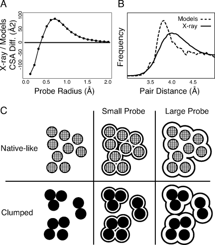
Differences in atomic arrangement in computational versus experimental structures. (A) The median difference in contact surface area between computationally generated structures and crystal structures for probe radii 0.1 to 2.0 Å in radius. The contact surface area is measured over 7 Å radius balls of atoms surrounding computed cavities. For probes 0.4 Å or larger, the computationally generated models have more exposed surface and crystal structures have more surface exposed to very small probes. (B) The RDF for methyl side chain groups in crystal structures and computationally generated protein structures. In crystal structures, the methyl groups are typically 4.0 Å apart but there is a broad peak. Methyl–methyl pairs in computationally generated models tend to be spaced slightly closer together and have a tighter peak around this value. (C) Model for differences in atom distributions for computed models (black) versus experimentally determined structures (grey). The outline represents the surface exposed to a small or large probe. The evenly packed configuration has more surface area exposed to a small probe while a large probe can access more surface area in the clumped arrangement. We hypothesize the clumped arrangement occurs more frequently in computationally generated structures.
We hypothesize that the differences between predicted models and crystal structures reflect clumping of atoms following minimization of pair-additive energy functions, such as the Rosetta fullatom energy. Figure 8(C) shows a hypothetical native-like, evenly spaced arrangement of atoms as shaded circles and a set of clumped atoms as filled circles. The surface accessible to both small and large probes is shown for both the native-like and clumped sets of atoms. For a small probe, there is more surface area exposed in the evenly distributed set of atoms because the even spacing is greater than the size of the probe in most places, but there is less exposed surface area in clumped arrangement because even a small probe cannot fit within the tight groupings. In contrast, for a large probe, there is less surface area exposed in the evenly distributed set of atoms and more exposed surface area in the clumped arrangement. The data shown in Figure 8(A,B) are well explained by this hypothesis.
The physical origins of the difference in packing between computationally generated and crystal structures may be twofold. First, the clumping observed in predicted and designed structures could reflect the missing entropic contributions associated with atomic vibrations during energy minimization (the energy rather than the free energy is being minimized). Second, the increased number of large voids in computed models likely reflects the limited extent to which solvation can be modeled with pair additive force fields. A large component to the free energy of solvation is the cost of forming a protein-sized void in the solvant, and this cavity free energy cannot be captured by a pair additive function. The importance of this contribution is illustrated by the very small number of voids in native protein structures, and the neglect of this term could explain the larger number of voids in computed models. Our new approach to quantifying packing is a step toward incorporating the solvent associated cavity free energy into protein structure prediction and design calculations. Toward this end, we are developing a differentiable RosettaHoles score, which can be easily minimized, for incorporation directly into modeling calculations.
The same kind of packing flaws found in computationally generated protein designs and structure predictions occur in some experimentally determined structures. Low-resolution X-ray and NMR structures, in particular, appear poorly packed in comparison to high-resolution X-ray structures. A systematic analysis of the PDB shows that many post-1990 packing quality outliers are problematic crystal structures. Our analysis of packing in the PDB has already lead directly to an author's request for retraction. Further, RosettaHoles is complementary to existing validation methods. We have compared the RosettaHoles score to the MolProbity score, an extensively used composite of many validation metrics including bond geometry and steric clashes.12 MolProbity and packing scores for 37,059 crystal structures in the PDB were compared, and the overall correlation is 0.527. Much of this correlation is due to the underlying resolution of the structures as both MolProbity and RosettaHoles scores are highly correlated with resolution. If the structures are divided into 0.5 Å resolution bins, the average correlation between the packing and MolProbity scores within each resolution bin is 0.203. This low correlation is reflective of the fact that the clashes and bond geometry features measured by MolProbity are largely independent of voids and underpacking measured by RosettaHoles. Because it provides new and valuable structural information, we believe RosettaHoles will help in the identification and correction (or retraction if corrections cannot be made) of other flawed structures as well as validation of new submissions to the PDB.
Methods
Overview
Our goal is to visualize and quantitatively measure underpacking in the protein core. RosettaHoles starts by finding the largest balls that can be placed in the empty space adjacent to each atom in the structure [Fig. 1(A)] and then prunes away balls that are accessible to a water-sized probe from the outside of the structure [Fig. 1(B)]. The remaining buried void-filling spheres are the basis for both visualization and quantitative analysis of core packing. For visualization, the spherical holes are clustered into contiguous cavities [Fig. 1(C)], and small holes/clusters are pruned away [Fig. 1(D)]. The resulting cavity clusters can then be displayed with a molecular visualization package such as RasMol or PyMol.13,14 Quantitative analysis is based on the contact surface area, the area that is accessible to probes of various sizes on the surface of an atom or group of atoms. The contact surface area statistics were used in a machine-learning-based packing measure that was trained and tested on sets of well packed and poorly packed structures. The data sets used for training included incorrect ab initio structure predictions with good Rosetta energy but poor packing, fixed-backbone protein designs that minimize Rosetta energy8 but tend to be poorly packed, and comparative models generated by Rosetta during the CASP7 experiment15 (www.predictioncenter.org). Testing was done on models submitted by all groups in CASP7 and on the whole of the PDB. The following sections describe the RosettaHoles methodology in detail.
Definition of cavities
For each atom Ai in the structure, we compute the largest empty ball Bi tangent to Ai that does not overlap any other atoms. This computation proceeds in three steps: (1) For each atom Ai of radius ri, define a set of 30 × 162 dots:  that are evenly distributed on concentric spheres of radius ri + pr centered on atom Ai (there are 162 dots on each concentric sphere; the dot mask for each concentric sphere is rotated randomly to more evenly sample the space around each atom). (2) Remove
  from Dots(Ai) if
  is closer to the surface of any other atom Aj≠i than it is to the surface of Ai. The resulting dot sets are a discrete approximation to an Apollonious diagram, a partitioning of space in which each atom is assigned a cell and all points in that cell are closer to the surface of that atom than to the surface of any other atom (see Fig. 2). (In the special case where all atoms are exactly the same size, the Apollonious diagram is the same as a Voronoi diagram.) (3) Select CSApr(
 ) which is furthest away from the surface of atom Ai, breaking ties arbitrarily. Figure 2 shows the results of a 2D implementation of this process performed on a slice through heat shock operon repressor HrcA. Shaded circles represent atoms and the surrounding like-colored dots are closer to that atom than any other (step 2). The furthest dot for each atom (step 3) is marked as a larger like-colored dot with a black center. The ball Bi of radius ri + pri centered on CSA3.0(
 ) will touch the surface of atom Ai (to within 0.1 Å) and will be the largest such ball (to within 0.2 Å) that does not intersect any other atom Aj≠i. The colored open circles in Figure 2 are the 2D analog of these spheres. This calculation can be performed quickly using precomputed bitmasks.16
For the balls to represent interior cavities, those on the surface must be removed. We define ball Bi to be buried if a probe sphere the size of a water molecule (1.4 Å) cannot touch Bi without intersecting any other ball Bj≠i or any atom Ai. Balls with any degree of exposure to a water-sized probe are removed. This process is repeated until no exposed balls remain; multiple rounds of pruning are required because the removal of one ball may expose another. Figure 1(A) shows heat shock operon repressor HrcA (PDB code 1STZ, an arbitrarily selected example) and its cavities in three different ways, a 2D slice with coloration representing depth, a 3D VDW structure, and a cartoon representation. Figure 1(B) shows the cavities in Figure 1(A) after pruning. Pruning is followed by clustering overlapping balls into cavities, as shown in Figure 1(C). For visualization, clusters that have joint volume less than 20 Å3 or surface area less than 40 Å2 are removed, resulting in a final set of cavities as illustrated in Figure 1(D). Packing statistics are computed for a representative set of the buried balls, as described later.
Packing statistics
The RosettaHoles scores are based on packing information about a cavity ball and the local region surrounding it, most importantly the contact surface area of atoms surrounding the cavity with respect to a sequence of probe radii, 0.1 Å, 0.2 Å, … 3.0 Å. To reduce computation time, a representative set of cavity balls is selected in a greedy fashion by successively choosing the largest such ball that is not within 4 Å of a previously selected ball. For each buried cavity ball Bi in the representative set, we record the radius, number of other balls Bi overlaps, and total volume and surface area of the cluster containing Bi. In addition to the holes themselves, we examine the contact surface area of portions of the protein structure surrounding each ball. Contact surface (accessible area on the atomic surface) was used in preference to solvent accessible surface (area swept out by the probe center) or molecular surface (a smoothed, continuous atomic surface) because contact surface area with respect to different probe radii are directly comparable: a smaller probe always has greater or equal contact surface area than a larger probe. For each void-filling ball Bi, define  to be the shell of atoms that are between r − 1.0 and r Å from the center of the cavity ball Bi. For each Bi, we consider the atomic shells CSApr(
 ) − CSA3.0(
 ) of radii {1.0 Å, 2.0 Å, … 7.0 Å} and compute the contact surface area (not including the cavity balls) of Dots(Ar) = {dot
 |k = 1,2,…162; pr = 0.1 Å, 0.2 Å, … 3.0 Å} for various probe sizes pr, denoted dot
 , and normalize by dot
 . This normalization corrects for atoms that are on the surface of the structure. Values reported for each dot
 ∈ Dots(Ai) are dot
 for pr = 0.1 Å, 0.2 Å, … 0.2.9 Å. A score for each representative cavity ball is generated from these raw statistics via an SVM, as described in the following section.
Assessment of packing quality
SVM description
The quantitative measures reported by RosettaHoles are based on an SVM trained to estimate the probability that a local cavity-centered region of a structure is from a high-resolution crystal structure versus a computationally generated model. The long vectors of packing statistics described in Packing Statistics section are condensed into summary statistics by taking a weighted average (linear combinations of individual statistics) with weights determined by linear kernel SVM, as described in the next section. To ease interpretation, the summary statistics are mapped monotonically to the interval [0,1] and thus can be interpreted roughly as probabilities. Predictions were performed using a soft margin SVM with a linear kernel and reported as empirical probabilities via a sigmoidal mapping17 as implemented in the R package e1071.18 We trained separate SVMs to (1) estimate the probability of an individual cavity-centered region being part of a crystal structure and (2) to estimate RMSD of a cavity centered region of a computational model to that of a crystal structure via an SVM regression.18 All training and prediction was done on individual cavities (approximately 400–1000 per structure). Aggregate probability and RMSDpred scores for whole structures are taken as the median score of all the local scores for the structure. Other more sophisticated methods of summarization, including mean and various quantiles, were tried, with no clear benefit over simply taking the median of the scores for each ball.
SVM training
SVM training was carried out on three data sets: (1) crystal structures for 45 small to medium sized proteins and corresponding high RMSD structure predictions that have low Rosetta fullatom energy but are poorly packed; (2) fixed-backbone redesigns of 59 proteins along with corresponding crystal structures; (3) homology models for 12 medium to large size CASP7 targets as well as the crystal structures for these targets. There is an overlap of eight proteins between sets (1) and (2), but no models were the same. The first two data sets were used to evaluate the ability of packing statistics to discriminate artificially generated protein structures of poor quality from their crystal structure counterparts. Set (3) was used in regression tests to predict local RMSD to crystal structure for each local atomic shell in computational models. Discrimination tests on sets (1) and (2) were cross-validated 10 fold and no models of the same protein sequence were included in both the training and test set. RMSD predictions on set (3) were tested using a 12-fold leave-one-out style cross validation by testing on structures from one protein and training on data from the other 11. For training sets larger than 10,000 examples, a random subset of size 10,000 was chosen for training (there are many computationally generated structures for each protein and many cavities per structure, yielding many examples).
Acknowledgments
We thank Phil Bradley for original ideas about contact surface area-based assessment of protein packing quality, John Karanicholas for help in development and debugging, and Andrew Ban for mathematical contributions. We thank Bin Qian, Rhiju Das, Srivatsan Raman, Paul Murphy, Divya Bhat, Lin Jiang, Andrew Lever-Fay, James Thompson, and others who have used RosettaHoles and provided feedback and Jane Richardson, Janet Smith, and other members of the PDB Validation Task Force for help in analysis of packing outliers. We thank Dale Tronrud and Brian Matthews for communicating their findings on the 179L structure. RosettaHoles is available as part of the Rosetta software package (http://www.rosettacommons.org/) and will soon be made available as a service on the Robetta web server (http://robetta.bakerlab.org/).
References
- 1.Kellis JTJ, Nyberg K, Fersht AR. Energetics of complementary side-chain packingin a protein hydrophobic core. Biochemistry. 1989;28:4914–4922. doi: 10.1021/bi00437a058. [DOI] [PubMed] [Google Scholar]
- 2.Erikson AE, Baase WA, Zhang XJ, Heinz DW, Baldwin EP, Mathews BM. Response of a protein structure to cavity-creating mutations and its relation to the hydrophobic effect. Science. 1992;255:178–183. doi: 10.1126/science.1553543. [DOI] [PubMed] [Google Scholar]
- 3.Eriksson AE, Baase WA, Wozniak JA, Mathews BM. A cavity-containing mutant of T4 lysozyme is stabilized by buried benzene. Nature. 1992;355:371–373. doi: 10.1038/355371a0. [DOI] [PubMed] [Google Scholar]
- 4.Lee B, Richards FM. The interpretation of protein structures: estimation of static accessibility. J Mol Biol. 1971;55:379–400. doi: 10.1016/0022-2836(71)90324-x. [DOI] [PubMed] [Google Scholar]
- 5.Liang J, Edelsbrunner H, Fu P, Sudhakar PV, Subramaniam S. Analytical shapecomputation of macromolecules: I. molecular area and volume through alpha shape. Proteins. 1998;33:1–17. [PubMed] [Google Scholar]
- 6.Liang J, Edelsbrunner H, Fu P, Sudhakar PV, Subramaniam S. Analytical shapecomputation of macromolecules: II. Inaccessible cavities in proteins. Proteins. 1998;33:18–29. [PubMed] [Google Scholar]
- 7.Boser BE, Guyon IM, Vapnik VN. A training algorithm for optimal margin classifiers. In: Haussler D, editor. 5th Annual ACM Workshop on COLT. Pittsburgh, PA: ACM Press; 1992. pp. 144–152. [Google Scholar]
- 8.Rohl CA, Strauss CE, Misura KM, Baker D. Protein structure prediction using Rosetta. Meth Enzymol. 2004;383:66–93. doi: 10.1016/S0076-6879(04)83004-0. [DOI] [PubMed] [Google Scholar]
- 9.Janssen BJC, Read RJ, Brünger AT, Gros P. Crystallographic evidence for deviating C3b structure. Nature. 2007;448:E1-E2. doi: 10.1038/nature06102. [DOI] [PMC free article] [PubMed] [Google Scholar]
- 10.Zhang XJ, Wozniak JA, Matthews BW. Protein flexibility and adaptability seenin 25 crystal forms of T4 lysozyme. J Mol Biol. 1995;35:527–552. doi: 10.1006/jmbi.1995.0396. [DOI] [PubMed] [Google Scholar]
- 11.Hooft RW, Vriend G, Sander C, Abola EE. Errors in protein structures. Nature. 1996;381:272. doi: 10.1038/381272a0. [DOI] [PubMed] [Google Scholar]
- 12.Davis IW, Leaver-Fay A, Chen VB, Block JN, Kapral GJ, Wang X, Murray LW, Arendall WB, III, Snoeyink J, Richardson JS, Richardson DC. MolProbity: all-atom contacts and structure validation for proteins and nucleic acids. Nucleic Acids Res. 2007;35:W375–W383. doi: 10.1093/nar/gkm216. [DOI] [PMC free article] [PubMed] [Google Scholar]
- 13.Sayle R, Milner-White EJ. RasMol: biomolecular graphics for all. TIBS. 1995;20:374. doi: 10.1016/s0968-0004(00)89080-5. [DOI] [PubMed] [Google Scholar]
- 14.DeLano WL. The PyMOL Molecular Graphics System. Palo Alto, CA, USA: DeLano Scientific LLC; 2008. http://www.pymol.org. [Google Scholar]
- 15.Proceedings of the Seventh Meeting on the Critical Assessment of Techniques for Protein Structure Prediction. Proteins. 2007;69(Suppl 8):1–207. doi: 10.1002/prot.21849. [DOI] [PubMed] [Google Scholar]
- 16.LeGrand SM, Merz KM. Rapid approximation to molecular surface area via the use of Boolean logic and look-up tables. J Comput Chem. 1993;14:349–352. [Google Scholar]
- 17.Platt JC. Probabilities for SV Machines. In: Smola A, Bartlett P, Schölkopf B, Schuurmans D, editors. Advances in large margin classifiers. MIT Press; 1999. pp. 61–74. [Google Scholar]
- 18.R Development Core Team. R: A language and environment for statistical computing. Vienna, Austria: R Foundation for Statistical Computing; 2008. http://www.R-project.org. [Google Scholar]
- 19.Drucker H, Burges CJC, Kaufman L, Smola A, Vapnik V. Support vector regression machines. InNIPSpp. Cambridge, MA: MIT Press; 1997. pp. 155–161. [Google Scholar]
- 20.Berman HM, Westbrook J, Feng Z, Gilliland G, Bhat TN, WeissigHelge, Shindyalov IN, Bourne PE. The Protein Data Bank. Nucleic Acids Res. 2000;28:235–242. doi: 10.1093/nar/28.1.235. [DOI] [PMC free article] [PubMed] [Google Scholar]
- 21.Lovell SC, Davis IW, III WBA, de Bakker PIW, Word JM, Prisant MG, Richardson JS, Richardson DC. Structure validation by C-alpha geometry: phi, psi, and C-beta deviation. Proteins. 2003;50:437–450. doi: 10.1002/prot.10286. [DOI] [PubMed] [Google Scholar]


