Computing generalized Langevin equations and generalized Fokker–Planck equations

Abstract

The Mori–Zwanzig formalism is an effective tool to derive differential equations describing the evolution of a small number of resolved variables. In this paper we present its application to the derivation of generalized Langevin equations and generalized non-Markovian Fokker–Planck equations. We show how long time scales rates and metastable basins can be extracted from these equations. Numerical algorithms are proposed to discretize these equations. An important aspect is the numerical solution of the orthogonal dynamics equation which is a partial differential equation in a high dimensional space. We propose efficient numerical methods to solve this orthogonal dynamics equation. In addition, we present a projection formalism of the Mori–Zwanzig type that is applicable to discrete maps. Numerical applications are presented from the field of Hamiltonian systems.

Many applications such as molecular dynamics lead to the solution of a system of ordinary differential equations,

involving a wide range of time scales. For example the time step in molecular dynamics simulations of proteins is 1 fs while typical events of interests are in the micro- or millisecond time scale. Carrying out these simulations using brute force techniques is impractical (e.g., by integrating the equations of motion); this is one of the main limiting factors towards greater predictability and applicability. This issue can be partially addressed by techniques that attempt to model this high-dimensional system by using a reduced set of resolved variables A(u), or observables. It is not possible to formulate exact equations for dA(t)/dt in closed form, that is in terms of A only. Approximations are necessary to close the equations. An effective approach can be derived from the Mori–Zwanzig formalism (1–3), which assumes that there is a probability distribution μ(du) conserved by the dynamics. This formalism leads to a decomposition of dA(t)/dt in three terms (4): a drift term that is a function of A(t), a memory term that depends on A(s) for 0 ≤ s ≤ t, and a fluctuating term F_t. One may then replace the fluctuating term by a stochastic process, for example white or colored noise (5, 6), to close the system of equations.

As examples of applications in biochemistry, one might be interested in modeling the position of an ion in a membrane channel, or the motion of the centers of mass of groups of atoms without resolving internal vibrations. It might also be desirable to model a large number of degrees of freedom which are computationally expensive to calculate; this is the case for example in implicit water models where water molecules are removed from the system and replaced by a stochastic model such as a Langevin model. Many other such examples can be found from the literature on multiscale modeling (5).

The same Mori–Zwanzig formalism can be used to derive a kind of generalized Fokker–Planck equation for the evolution of a probability density function ϕ^t(A). This equation, contrary to the Fokker–Planck equation for diffusive processes, contains a term function of ϕ^t and a non-Markovian term function of past values ϕ^s, 0 ≤ s ≤ t. We will show how all the relevant time scales in the system, e.g., reaction rates, and metastable basins can be extracted numerically from this equation.

One of the main numerical difficulties in these equations is that the fluctuating term F _t and the memory kernels require in principle the solution of the so-called “orthogonal dynamics equation” (7) which is a partial differential equation with n + 1 variables (recall that u ∈ ℝⁿ). This is impractical in most real life applications where n can be in the range 10⁴ – 10⁶. Many techniques have been developed to address this issue (see refs. 5 –8 for example). We propose a new approach to solve this equation. This approach does not require a time scale separation, wherein the variable A is assumed to be much slower than other time scales in the system, or an adiabatic or Markovian approximation. The method is numerically robust, e.g., it is not sensitive to small perturbations in the data (see for example ref. 9 which requires solving a Volterra integral equation of the first kind). The method has a low computational cost and can be carried out on desktop computers.

The paper is organized as follows. We first present the standard Mori–Zwanzig formalism. For any phase variable B, this gives an equation for e^tLB where $L\stackrel{def}{=}{\displaystyle {\sum }_{i=1}^n{R}_i\partial /\partial u_i}$ is the Liouvillian. We also derive a new formulation applicable to a discrete map M, in which we obtain equations for M^k B. This is followed by 2 important equations which can be derived from the Mori–Zwanzig formalism: the generalized Langevin equation (GLE) and generalized non-Markovian Fokker–Planck equation (GFPE). A numerical discretization of the GFPE based on a Galerkin scheme is then proposed along with an algorithm to calculate reactions rates and other time scales in the system. These equations rely on the solution of the orthogonal dynamic equations. An algorithm to carry out this calculation is presented. The paper ends with numerical results. The notation $\stackrel{\text{def}}{=}$ indicates a definition or an equality that cannot be derived from previous statements.

Mori–Zwanzig Projection

We consider the dynamical system given by Eq. 1 where u ∈ Ω ⊆ ℝⁿ. In the context of molecular dynamics of proteins, the vector u is the set (q,p) of atom coordinates and momenta. In many contexts it is desirable to model the dynamical system using only a subset of variables instead of the full set u. This might be the case if one is trying to build a coarse grained model. These problems can be formulated abstractly in the following fashion. Let us denote υ(u ₀,t) the solution of Eq. 1 at time t with initial conditions u(0) = u ₀. A phase variable A is an m-dimensional vector valued function defined on Ω, A(u). Associated with the Liouvillian L, we define a time evolution operator e^tL : [e^tL A](u)$\stackrel{\text{def}}{=}$A(υ(u,t)).

The general model reduction problem or coarse graining problem can be formulated as follows: given a phase variable B and e^sLA (0 ≤ s ≤ t), is it possible to approximate e^tLB? We call this the closure problem. For example, B could be dA/dt. This problem is trivial if A is a complete set of generalized coordinates, i.e., m = n. In most applications however, m ≫ n, so that this (coarse-graining) procedure may provide significant computational speed-up.

The Mori–Zwanzig procedure is a very general and powerful formalism to help answer such problems. From now on, we assume that the initial conditions for u are drawn from a probability distribution μ⁰. The probability distribution μ^t is defined by the condition

We will assume that μ^t is conserved by the dynamics, i.e., μ^t = μ⁰. We now simply denote this measure by μ.

Standard Mori–Zwanzig Decomposition.

The Mori–Zwanzig procedure uses a projector operator P. We define P as the following conditional expectation (4):

We say that the phase variable C is a function of phase variable D if D(u) = D(u*) implies C(u) = C(u*). As an example PB is a function of A.

Because the Mori–Zwanzig decomposition has been derived by many authors (1, 4), we skip the derivation and simply state the final formula. We define the phase variable F _t (fluctuating term) as the solution of the following partial differential equation with n + 1 variables, the orthogonal dynamics equation:

Then:

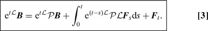For later convenience, we denote S_⊥ ^τ the evolution operator associated with the orthogonal dynamics equation:

A key point to observe in Eq. 3 is that e^tLPB is a function of e^tL A, and e^tLPLF _s is a function of e^tL A. This means that given e^sL A, 0 ≤ s ≤ t, we can calculate e^tLPB and ∫₀ ^t e^{(t – s)L}PLF _sds without knowing the fully resolved trajectory υ(u,t). In this sense, the first 2 terms in the decomposition satisfy the closure problem. The function e^{(t – s)L}PLF _s is often called the memory kernel because it is a function of past values of A. In addition, the last term satisfies PF _t = 0 for all t, and may therefore be called the fluctuating term.

Discrete Mori–Zwanzig Decomposition.

It is possible to derive a similar looking Mori–Zwanzig decomposition where the continuous integration over time is replaced by a discrete sum. This decomposition can be useful in different contexts, when the data itself is discrete, or when a discretization is applied in numerical computation. For example, the set Ω might be divided into N ^cell cells and the data A(u) could be given as a vector of length N ^cell such that A _i = 1 if u is in cell i and 0 otherwise. The discrete Mori–Zwanzig decomposition can be formulated using an arbitrary map M : u ↦ Mu. For any phase variable A, we define: MA : u ↦ A(Mu). As a typical example, M can be defined as M $\stackrel{\text{def}}{=}$ e^ΔtL. Let us define F _k recursively by

The following decomposition can be obtained for an arbitrary phase variable B, with k ≥ 1 an integer:

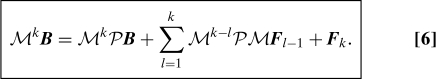This decomposition is in the same spirit as the original Mori–Zwanzig decomposition because it satisfies the following properties: PB and PMF _l are functions of A, and PF _k = 0. It can be proved by induction.

Generalized Langevin Equations

The Mori–Zwanzig decomposition can be further transformed to reach a form more suitable to construct stochastic models of A. In particular, this leads to a generalized Langevin equation (10). If we assume that the dynamics is volume preserving (∇ · R $\stackrel{\text{def}}{=}$ 0), then, using integration by parts and the chain rule, the memory kernel PLF _t can be shown to be equal to

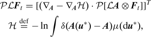where ^T is the transpose operator and ⊗ is the outer product of 2 vectors. Using this result with B $\stackrel{\text{def}}{=}$ LA along with the Mori–Zwanzig decomposition (Eq. 3), we get a form of the fluctuation dissipation theorem (11, 10):

where the memory kernel is related to the autocorrelation of the fluctuations F _t.

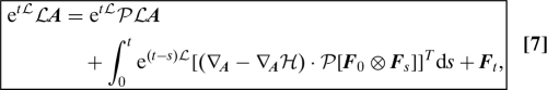
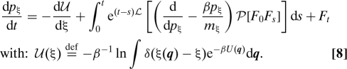
This equation can be further simplified to some of the usual forms. We briefly discuss an example. Consider the case of a separable Hamiltonian system H $\stackrel{\text{def}}{=}$K(p) + U(q), in the canonical ensemble (β $\stackrel{\text{def}}{=}$ (k _B T)⁻¹), with atomic positions q _l, momenta p _l, and masses m _l. We may choose A to be a coordinate and its momentum (ξ,p _ξ). For simplicity we further assume that the mass $m_{\xi }^{-1}\stackrel{\text{def}}{=}{{\sum }_l\frac{1}{m_l}\left(\frac{\partial \xi }{\partial q_l}\right)}^2$ is constant. From Eq. 7, we can prove that the equations of motion are then given by dξ/dt = p _ξ/m _ξ, and

Fokker–Planck Equation

We now derive a Fokker–Planck equation for the resolved variable A. We have to distinguish between variable A seen as a function of u, which is denoted by A(u), and seen as an independent variable, then denoted A. We apply the Mori–Zwanzig projection (Eq. 3) to the scalar phase variable B _a $\stackrel{\text{def}}{=}$ Lδ(A(u) − a):

We denote ϕ^∞(a) the equilibrium probability density function of a = A(u). The Fokker–Planck equation assumes a simple form if we choose an initial probability distribution of the form

where ϕ⁰ is some given initial condition. This corresponds to a constrained equilibrium where variables orthogonal to a are sampled from the equilibrium distribution while a is sampled according to ϕ⁰. We denote ϕ^t(a) the probability density function corresponding to the initial probability distribution ν⁰(du).

To obtain a Fokker–Planck equation, we need to multiply Eq. 9 by ν⁰(du) and integrate over u. Using the chain rule, integration by parts and properties of the Dirac δ functions (a long derivation), we can show that this leads to a GFPE:

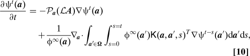where ψ^t $\stackrel{\text{def}}{=}$ ϕ^t/ϕ^∞, and K is a tensor phase-variable:

The notation P_a′ indicates explicitly the value of A(u) = a′ used in the projection.

Numerical Solution Using a Galerkin Discretization

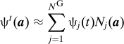
We now discuss how the GFPE may be solved numerically. The direct numerical calculation of the memory kernel K(a,a′,s) is difficult because of the Dirac δ function in its definition (Eq. 11). However this becomes relatively straightforward if one uses a Galerkin discretization of ψ^t. Suppose we have some basis functions N _j(a) and:

Galerkin Discretization.

The Galerkin formulation is derived from Eq. 10 by multiplying by the test function N _i(a) and integrating over a. The coefficients ψ_i(t) are then solutions of the following set of integro-differential equations.

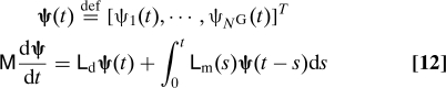with the following matrices:

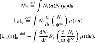For irreversible processes, [L_m(s)]_ij decays when the support of N _i and N _j are far from one another (diagonally dominant matrix) or when s is large.

Discrete Mori–Zwanzig Decomposition.

A second formulation can be obtained by taking advantage of the discrete Mori–Zwanzig formalism (Eq. 6). We choose as M the time evolution operator over Δt : M $\stackrel{\text{def}}{=}$ e^ΔtL and as B _a the scalar phase-variable (M − I)δ(A(u) − a). Then, we obtain the following scheme (t _k = kΔt):

where

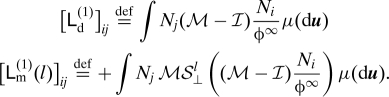The notation S_⊥ ^l refers to the discrete orthogonal dynamics defined by Eq. 5. The integer superscript and the context are hopefully sufficient to remove the ambiguity with S_⊥ ^s from Eq. 4.

This decomposition is not a finite-difference approximation in time. In particular it gives exactly the same solution as Eq. 12 at times kΔt. There is no time discretization error. This is because the discrete decomposition (Eq. 6) is an exact equation.

This formulation does not require any derivative of N _i and therefore is also applicable for discontinuous basis functions such as the hat function. (N _i(x) = 1 if 0 ≤ x ≤Δ x and 0 otherwise.) A simple piecewise constant approximation of ψ is therefore possible. This makes the numerical implementation relatively simple. This numerical scheme was chosen for the discussion in Numerical Results.

Reaction Rate and Metastable Basins.

In many chemical systems, metastable basins are separated by energy barriers making transition a rare event. Calculating the rate of transition between these basins is often of great importance. Let us consider Eq. 13, and look for solutions of the form ψ(t _n) $\stackrel{\text{def}}{=}$ μ_l ⁿψ_l. From these solutions, we will derive the general solution of our problem. Plug in the form of our solution in Eq. 13 and assume that the memory kernel L _m ⁽¹⁾(l) becomes negligible for l ≥ l ₀. Then, we obtain a polynomial eigenvalue problem

All solutions to this equation can be associated with solutions of Az = μBz with

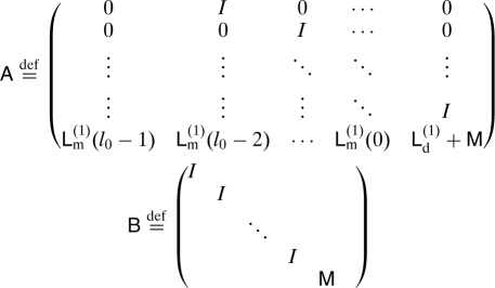and z ^T = (ψ^T,μψ^T,…,μ^l₀ψ^T). If we assume that the eigenvalue problem Az = μBz admits N ^G(l ₀ + 1) distinct eigenvalues μ_l and eigenvectors z _l, we can form the general solution of our problem. Consider the vector

for a given initial condition ψ(t ₀). It can be expanded in the basis z _l : z(t ₀) = ∑_{l = 1} ^NG(l₀+1) c _l z _l. By induction and using Eq. 13, we can prove that the general solution is of the form z(t ₀) = ∑_{l = 1} ^NG(l₀+1) c _l(μ_l)ⁿ z _l, and in terms of ψ:

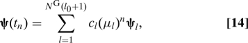where ψ_l is the vector formed by taking the first N ^G components of z _l. Note that the ψ_l are not linearly independent because they are in a space of dimension N ^G but we do need N ^G(l ₀ + 1) such vectors to expand the general solution.

In many chemical reactions, there is a (or a few) time scale that is very slow compared to the other time scales in the system. This is the case for example when an energy barrier separates two metastable basins. That time scale can be obtained from μ_l. One of the eigenvalues must be equal to 1 and the corresponding eigenvector ψ₀ is the equilibrium distribution. All others eigenvalues in general have a real part in the interval] −1,1[. In many instances, there is a single (or a few) eigenvalue μ₁ close to 1; this is the slowest time scale in the system. The corresponding reaction rate is given by −ln(μ₁)/Δt. This is the rate of transition across the energy barrier separating the 2 most stable basins. The eigenvector ψ₁ is approximately constant in each metastable basin but changes sign between basins. The change of sign can be used to identify precisely the boundary of metastable sets (for additional details see ref. 12 for example). This is illustrated in Numerical Results. More generally, all time scales in the system can be extracted from the eigenvector decomposition, for example the first passage times. If needed the conditional probability p(a,t|a ₀,0) can be obtained.

Orthogonal Dynamics Equation

Both the GLE and GFPE require computing the solution of the orthogonal dynamics equation, which is a partial differential equation in dimension n + 1. A direct solution is impractical in most cases. Various strategies with low computational cost have been proposed most notably by Lange et al. (9) and Chorin et al. (7). In ref. 9, the authors reconstruct the memory kernel in the GLE from the velocity autocorrelation; their equation is derived from Eq. 8 assuming that P[F ₀ F _s] is independent of p _ξ. This leads to a Volterra integral equation of the first kind which is difficult to solve numerically. In ref. 7, a computationally efficient scheme is proposed to calculate PLF _s using a Galerkin approach.

We now assume that we have a numerical algorithm, e.g., Molecular Dynamics or Monte-Carlo, that allows generating samples u with a distribution equal to (close to) the equilibrium distribution μ. We define the following notations. N ^sam: number of sample points u; u ₀ ^k: sample k; N ^G: number of basis functions N _i(a); N ^mem: number of discrete times s at which the memory term is computed. Assume we integrate in time using some numerical procedure; we denote u _m ^k the sample at step m, using u ₀ ^k as initial condition.

Given a function G, there are several ways to numerically approximate PG from G(u ₀ ^k). For our application, we consider a Galerkin expansion of the form P^G G(a) $\stackrel{\text{def}}{=}$ ∑_j P _j N _j(a) with

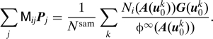The pseudocode to numerically compute F _s is then given by For l = 0 to N ^mem − 2, do Calculate P^G G with G(u ₀ ^k) = F _l(u ₁ ^k) Calculate F _l+1(u _m ^k) = F _l(u _m+1 ^k) − (P^G G)(A(u _m ^k)), for 0 ≤ m ≤ N ^mem − 2 − l

This is a numerical implementation of Eq. 5 where M is the evolution operator e^ΔtL. In the limit of taking Δt → 0, the sequence F _k in Eq. 5 (0 ≤ k ≤ t ₁/Δt) converges to F _kΔt in Eq. 2; the single step error is O(Δt ²). It is possible to derive higher order integrators, however, in practice, statistical errors incurred when approximating P are larger than the time discretization errors. The cost of this calculation is O(N ^sam(N ^mem)²). If we apply this to calculate the matrices in Eq. 12 or 13, the total cost is O(N ^sam(N ^mem)² N ^G). This assumes that the basis N _i has local support. If the basis has global support, e.g., Legendre polynomials, the total cost is O(N ^sam(N ^mem)² N ^G + N ^sam N ^mem(N ^G)²).

In the presence of energy barriers, it is possible to generate samples u ₀ ^k from the constrained ensemble, that is for various a ₀ we generate samples lying on the surface A(u) = a ₀. This is sufficient to calculate P^G and the efficiency of the method becomes independent of ϕ^∞(a) and in particular of energy barriers along A(u). If the system does not exhibit large energy barriers, it is possible to carry out this calculation using a single (a few) very long trajectory. In that case the total cost using our approach is reduced to O(N ^sam N ^mem N ^G) for a basis with local support.

Accuracy and Limitations

The method works irrespective of energy barriers along A(u). However it relies on techniques to numerically estimate P. This requires being able to efficiently sample the surface A(u) = a. Roughly speaking, if the coordinates orthogonal to A contain metastable basins, the number of steps in a molecular dynamics simulation required to generate N ^sam uncorrelated points is very large. A precise statement is beyond the scope of this paper and depends in general on the rate of decay of the auto-correlation of B when moving on the surface A(u) = a. If we consider a simulation in the hypersurface A(u) = a, the previous analysis (see Reaction Rate and Metastable Basins) shows that the number of steps required should be proportional to −1/ln(max_aμ₁ ^⊥(a)), where μ₁ ^⊥(a) is the largest eigenvalue different from 1 for the constrained dynamics with A(u) = a. In this case, specific acceleration techniques must be applied. We mention the technique of Zheng et al. ((13), biasing force along ∇A and ∇F _A), normal mode approximations (14), biasing techniques, etc. These techniques allow lowering max_aμ₁ ^⊥(a) away from 1.

We also note that the method will be computationally expensive to apply to problems where the dimensionality of A is large. This is because all the functions of A become difficult to discretize in an efficient manner. Techniques like sparse grid of Smolyak (15) may become useful in those cases.

Numerical Results

Oscillators.

It is possible for some systems to calculate analytically the fluctuating term F _t. We will use such a system to check the accuracy of Eq. 5 and the pseudo-code above. Consider the case of a particle attached to some masses with springs:

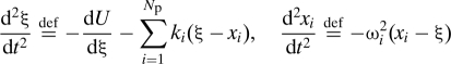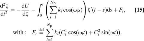
We can derive the following equation for ξ″ (5):

If we assume that the initial positions and momenta of the masses x _i are generated randomly according to the canonical distribution at temperature T (= (k _Bβ)⁻¹), then $C_i^1=1/\sqrt{\beta k_i}{\eta }_i$, $C_i^2=1/\sqrt{\beta k_i}{\zeta }_i$, with η_i and ζ_i normally distributed variables with variance 1 and mean 0. Consequently,

This is consistent with Eqs. 8 and 15.

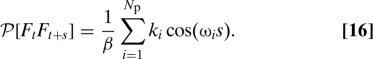
To demonstrate the accuracy of Eq. 5 and its correspondence with Eq. 2, we use Eq. 5 to calculate F _t (using the pseudo-code above) and then calculate P[F _t F _t+s] as a function of s. The result is compared with the analytical expression given by Eq. 16. Choose for example N _p = 32 particles with ω_i = i, k _i = 1. As the number of particles goes to infinity, P[F _t F _t+s] approximates a Dirac δ function at 0. Fig. 1 shows a comparison of Eqs. 5 and 16. We used a trajectory with 4 10⁷ steps and a step size of 5 × 10⁻³. The trajectory was generated using Langevin dynamics with a friction coefficient of 0.05 and a temperature of k _B T = 1. We note that the decay of the memory kernel happens on a time scale comparable to the time scale of ξ, and therefore the adiabatic approximation does not apply.

Fig. 1.

Oscillators with ω_i = i and k _i = 1. The numerical solution is compared with an analytical expression (Eq. 16). Eq. 5 and the pseudocode in Orthogonal Dynamics Equations were used.

Implicit Water Model.

It is common in molecular dynamics simulations of solvated molecules (e.g., protein) to model water using an implicit model. In that case, the water molecules are removed from the system and replaced by a model; the mean force may be estimated using various techniques such as the Poisson–Boltzmann equation or the Born and Onsager models (16). The fluctuating part is typically approximated by a Langevin term with friction and white noise. We revisit this problem using our approach.

We chose a small poly-peptide (alanine dipeptide) in water. This is a 22-atom molecule. We used 450 water molecules. The box size was 25.1 × 24.5 × 23 Å. We considered the total atomic force that water is exerting on the protein and A is the location of the center of mass of the protein. The memory kernel β/mP[F ₀ F _s] (see Eq. 8) is shown on Fig. 2.

Fig. 2.

(A) Memory kernel β/mP[F ₀ F _s] (see Eq. 8) for fluctuating atomic forces exerted on a protein by water molecules. (B) Derivative of the velocity auto-correlation function. We plot the left and right hand sides of Eq. 17 as an indirect way to verify our computation of P[F ₀ F _s.

In that case, we could not compare with a reference solution. However the following indirect verification was conducted. In Eq. 8, if we multiply by p(0), average over all initial conditions, and neglect the derivative with respect to p (see ref. 9), we get

As a way to verify our calculation of P[F ₀ F _s], we plot the left and right hand sides of Eq. 17 in Fig. 2. The agreement is very good.

Non-Markovian Fokker–Planck Equation.

We tested our numerical scheme to calculate the GFPE. A comparison with a direct brute force calculation is made. We used the discrete Mori–Zwanzig scheme described in Discrete Mori–Zwanzig Decomposition.

Consider a particle x in a double well potential given by x ²/4(x ² − 2). This function has 2 minima at −1 and 1, and a local maximum at 0. We attached to the particle 16 other particles using springs, with stiffnesses chosen such that the kernel P[F _t F _t+s] decays approximately like e^−20s (see Eq. 16 and ref. 5). The temperature was chosen such that k _B T = 0.1. This corresponds to a barrier of 2.5 k _B T. We generated trajectories using a Langevin equation with a friction of 1. The time step for the integration was 0.001. The time interval Δt (see page 3) is equal to 0.256. In our implementation of Eq. 13, we did not generate a single long trajectory as this would have resulted in poor statistics near −2 and 2. Instead we created bins of size 0.0625 and in each bin we generated a fixed number of initial conditions drawn from the constrained canonical ensemble distribution. For each initial condition, we ran a trajectory of length 16Δt = 4096 steps. This algorithm generated accurate data with small statistical errors.

After computing the drift matrix L_d ⁽¹⁾ and the memory matrices L_m ⁽¹⁾(l), we solved the GFPE numerically and compared with a brute force calculation. The initial conditions are taken from a Gaussian distribution centered at −1 with standard deviation 0.2. Trajectories were run with these initial conditions and the final value of x was recorded after 32,768 steps. This corresponds to 128Δt. The resulting probability density functions are shown on Fig. 3.

Fig. 3.

Probability density functions (PDF) at time 16Δt = 4.1. The label “PDF at t = 0 ” corresponds to the initial distribution of x. The label “Direct simulation” corresponds to an estimate of the PDF based on running many trajectories using Langevin dynamics. The label “Fokker–Planck” corresponds to the solution computed using Eq. 13. The label “Equilibrium” is the reference equilibrium distribution of x. The variable x is on the horizontal axis.

We computed the eigenvectors and eigenvalues of the polynomial eigenvalue problem as described in the section “Reaction rate and metastable basins.” One of the eigenvalues was found to be almost equal to 1. The corresponding eigenvector matched the equilibrium distribution. The second eigenvalue is 0.9946. The third is 0.84 and the other eigenvalues have a smaller real part. In Fig. 4, we plot the vector ψ₁ (see Eq. 14). As described in Reaction Rate and Metastable Basins, we expect this vector to change sign at the transition region between the 2 metastable basins, x < 0 and x > 0. This is the case; we computed that the 0 of the function is near x = 0.001.

Fig. 4.

Eigenvector ψ₁ vs. x _i. The eigenvalue for ψ₁ is 0.99462. The 0 of the function separates the 2 metastable basins.

In addition the associated eigenvalue gives a rate equal to −ln(μ₁)/Δt = 0.021 [time unit]⁻¹. We compared this rate with an estimate based on the brute force calculation shown in Fig. 3 (solid curve): This gave 0.021 [time unit]⁻¹. The transition state theory from ref. 17 predicts a rate of 0.033 [time unit]⁻¹, which is consistent with the fact that a rate from transition state theory overestimates the actual rate since re-crossing of the transition region at x = 0 is not accounted for.

In Fig. 5, we calculated the rate using the Fokker–Planck equation while varying the number of terms we keep in the memory kernel, that is for a given integer l on the x axis we only keep the terms L_m ⁽¹⁾(0),…,L_m ⁽¹⁾(l − 1). Fig. 5 shows the effect of the memory kernel on the rate, which is essentially multiplied by 3.5 when we keep 10 terms in the memory kernel. For l > 9, the memory kernel L_m ⁽¹⁾(l) is small and dominated by statistical noise. This plot shows the importance of memory and the non-Markovian effects in the evolution of ϕ^t.

Fig. 5.

Reaction rate, or rate of transition, vs. number of terms kept in the memory sequence L_m ⁽¹⁾(l). The direct simulation estimate is the horizontal line and is equal to 0.021.

Conclusion

We presented a theoretical framework and numerical techniques to calculate generalized Langevin equations and non-Markovian Fokker–Planck equations by sampling trajectories. A discrete form of the Mori–Zwanzig formalism has been derived (Eq. 6). A generalized non-Markovian Fokker–Planck equation was presented in a general setting (Eq. 10), along with its numerical discretization (Eq. 13). An algorithm to calculate the various terms in these equations is given. An important element is the procedure used to solve the orthogonal dynamics equation numerically. The accuracy of the method was shown with different examples, including one with analytical solutions, one with atomic forces exerted by water molecules on a polypeptide, and a problem with 2 metastable basins for the Fokker–Planck equation. We haven't addressed the question of estimating statistical errors, and cases with large energy barriers.

References

- 1.Mori H. Transport, collective motion, and Brownian motion. Prog Theo Phys. 1965;33:423–455. [Google Scholar]
- 2.Zwanzig R. Nonequilibrium Statistical Mechanics. New York: Oxford Univ Press; 2001. [Google Scholar]
- 3.Evans D, Morriss G. Statistical Mechanics of Nonequilibrium Liquids. London: Academic; 1990. [Google Scholar]
- 4.Chorin AJ, Hald OH, Kupferman R. Optimal prediction and the Mori–Zwanzig representation of irreversible processes. Proc Natl Acad Sci USA. 2000;97:2968–2973. doi: 10.1073/pnas.97.7.2968. [DOI] [PMC free article] [PubMed] [Google Scholar]
- 5.Givon D, Kupferman R, Stuart A. Extracting macroscopic dynamics: model problems and algorithms. Nonlinearity. 2004;17:R55–R127. [Google Scholar]
- 6.Berkowitz M, Morgan JD, McCammon JA. Generalized Langevin dynamics simulations with arbitrary time-dependent memory kernels. J Chem Phys. 1983;78:3256–3261. [Google Scholar]
- 7.Chorin AJ, Hald AH, Kupferman R. Optimal prediction with memory. Physica D. 2002;166:239–257. [Google Scholar]
- 8.Akkermans RLC, Briels WJ. Coarse-grained dynamics of one chain in a polymer melt. J Chem Phys. 2000;113:6409–6422. [Google Scholar]
- 9.Lange O, Grubmüller H. Collective Langevin dynamics of conformational motions in proteins. J Chem Phys. 2006;124:214903. doi: 10.1063/1.2199530. [DOI] [PubMed] [Google Scholar]
- 10.Akkermans RLC. New Algorithms for Macromolecular Simulation. Vol. 49. Berlin: Springer; Lecture Notes in Computational Science and Engineering; pp. 155–165. [Google Scholar]
- 11.Ciccotti G, Ryckaert J-P. On the derivation of the generalized Langevin equation for interacting Brownian particles. J Stat Phys. 1981;26:73–82. [Google Scholar]
- 12.Schütte C, Fischer A, Huisinga W, Deuflhard P. A direct approach to conformational dynamics based on hybrid Monte Carlo. J Comp Phys. 1999;151:146–168. [Google Scholar]
- 13.Zheng L, Chen M, Yang W. Random walk in orthogonal space to achieve efficient free-energy simulation of complex systems. Proc Natl Acad Sci USA. 2008;105:20227–20232. doi: 10.1073/pnas.0810631106. [DOI] [PMC free article] [PubMed] [Google Scholar]
- 14.Sweet C, Petrone P, Pande V, Izaguirre JA. Normal mode partitioning of Langevin dynamics for biomolecules. J Chem Phys. 2008;128:145101. doi: 10.1063/1.2883966. [DOI] [PMC free article] [PubMed] [Google Scholar]
- 15.Smolyak SA. Quadrature and interpolation formulas for tensor products of certain classes of functions. Dokl Akad Nauk SSSR. 1963;4:240–243. [Google Scholar]
- 16.Leach A. Molecular Modelling: Principles and Applications. 2nd Ed. New York: Prentice Hall; 2001. [Google Scholar]
- 17.Chandler D. Introduction to Modern Statistical Mechanics. 1st Ed. Oxford: Oxford Univ Press; 1987. [Google Scholar]