The kinetics of helix unfolding: Molecular dynamics simulations with Milestoning

Abstract

The unfolding process of a helical heteropeptide is studied by computer simulation in explicit solvent. A combination of a functional optimization to determine the reaction coordinate and short time trajectories between “Milestones” is used to study the kinetic of the unfolding. One hundred unfolding trajectories along three different unfolding pathways are computed between all nearby Milestones providing adequate statistics to compute the overall first passage time. The radius of gyration is smaller for intermediate configurations compared to the initial and final states suggesting that the kinetics (but not the thermodynamics) is sensitive to pressure. The transitions are dominated by local bond rotations (the ψ dihedral angle) that are assisted by significant nonmonotonic fluctuations of nearby torsions. The most effective unfolding pathway is via the N-terminal.

Introduction

The phenomenon of peptide dynamics has been the subject of intensive studies from both experimental and theoretical perspectives. Computer simulations have the potential to provide a wide range of information about this process, yielding microscopic insight into the pathways and rates of conformational transitions, including the characterization of rarely sampled intermediates ^1,2. The progress in computational studies of peptide dynamics and folding may be divided into several stages, with progressive improvements in methodology and investigations of larger systems. Early studies used direct MD and free energy simulations of secondary structure elements ¹, followed by extensive simulations of helices, sheets and mini-proteins with first implicit and later explicit solvent models ^1,2.

Early studies included following unfolding of helices and turns, performed at elevated temperatures or with umbrella sampling ^1,3. These simulations found individual helical hydrogen bond breaking occurring at tens to hundreds of picoseconds and stabilities of sheets significantly greater than for helices. Pioneering work involved 2.2 ns length explicit solvent MD trajectories of YPDGV, a turn-forming pentapeptide, for which folding and unfolding was found on the nanosecond time scale ⁴ and clustering was applied to analyze the conformational space and structural transitions⁵. Other studies employed the LES methodology for more comprehensive exploration of conformational space and determination of peptide structures CHDLFC⁵, and SYPFDV⁶ illustrating significant correlation between experimental structure and optimized peptide conformations.

More extensive calculations were initially performed using implicit solvation². For the blocked (AAQAA)₃ peptide, microsecond simulations with a solvent model involving a distance-dependent dielectric function and a solvent accessible surface area term described the conformational free energy surface and folding as a function of temperature⁷. A single free energy minimum was found at all studied temperatures, corresponding to a folded state in the low temperature range, and an unfolded state at higher temperatures. Cluster analysis showed that folding proceeded through multiple nucleation events. Simulations by Duan and coworkers using the Generalized Born (GB) implicit solvent model suggested that folding of alanine-rich helical peptides proceeded through several stages: three stages for the blocked YG(AAKAA)₂ AAKA peptide⁸ and two for the Fs-21 peptide, AAAAA(AAARA)₃A,⁹. Important results for folding of helices, sheets and small proteins were obtained using REMD². These studies showed that explicit solvent REMD can correctly predict the global free energy minima for small model helix-forming¹⁰ and hairpin-forming peptides^11,12, and others¹³. Good agreement between the calculated and observed melting temperature of Fs was obtained after adjustment of the AMBER force field¹⁰. The timescales for hairpin formation were estimated to fall in the microsecond range using energy landscape theory¹¹. REMD with the GB/SA implicit solvation gave incorrect results in some cases, predicting a helix-turn-helix structure for Fs and hydrophobic residues on the surface for the harpin-forming GB1 peptide². In our joint experimental-computational study of the WH21 peptide¹⁴ we found generally good agreement between the GB/SA REMD simulations employing the CHARMM¹⁵ force field and measured properties. The simulations found that the alpha-helix was the system free energy minimum at low temperatures, and predicted an enthalpy change of -10 kcal/mol and an entropy change of -30 cal/mol K^-1 for the folding transition, quite similar to the experimental values of -11.6 kcal/mol and -39.6 cal/(mol K)¹⁴.

Significant progress in enhancing the rate of conformational exploration was achieved with introduction of the replica exchange MD (REMD) method^2,16. REMD aims at thermodynamics and not at kinetics, which is the focus of the current investigation. Recent techniques to study kinetics include hyperdynamics^17,18, transition path sampling¹⁹ and sampling biased along an order parameter such as the TIS²⁰, PPTIS²¹, Forward Flux²² and Milestoning²³.

Current computer power enables simulations of folding equilibrium of peptides in aqueous solution using molecular dynamics (MD). Examples are a beta-hexapeptide²⁴, CW1 and CW2²⁵ and Ala5²⁶. With application of highly distributed computing systems, a significantly longer peptide, the 21-residue Fs system, has been studied²⁷. The overall picture is that methods for equilibrium simulations are well developed, with accuracy limited by potential function development^2,27, while a systematic computational description of peptide folding kinetics is only beginning to emerge.

In the present manuscript we use the reaction path approach (RP). Reaction Path (RP) studies of kinetics and thermodynamics of peptide conformational transitions were initiated by Czerminsiki and Elber^28,29 and were (significantly) exploited further by Wales³⁰. A variant of the peptide we investigate in the present manuscript was studied by stochastic path optimization by Cardenas and Elber³¹. Comprehensive sampling of conformational space is simpler in the RP approach compared to Molecular Dynamics (MD) simulations. However significant questions remain. Lack of explicit solvent, inaccuracies of the models for effective solvation (especially for kinetics), and the use of energy minima (with implicit solvent) instead of free energy add to the uncertainties of these investigations.

Milestoning^23,32-35 aims to solve some of the RP problems by combining features of RP and MD. Short time trajectories are computed in the neighborhood of the reaction coordinates and a coarse grained stochastic model for the motions is developed²³. This strategy makes it possible to investigate the kinetics in much larger systems³⁴. In the present manuscript our efforts focus on early events in the unfolding of a helical peptide. Unfolding is more appropriate for a study with the reaction path approach than folding. This is because, close to the unfolded state, the number of alternative conformations is large and the reaction coordinates create a large network. The network of unfolded structures is dense and more difficult to describe with few reaction coordinates. The conformations closer to the folded state and states lower in free energy are likely to be sparse and accessible to this approach as suggested also from analysis of a very large number of trajectories²⁷. Future studies will address more comprehensive structure of the folding network.

II. Theory

Reaction paths

The question of how to choose a reaction path (RP) to describe a complex condensed phase problem is an important challenge that attracted and continues to attract timely research. There are two reasons for the significant interest in RP. The first is of qualitative understanding of the reaction progress, and the second is of quantitative comparison to experimental data.

Atomically detailed simulations retain the coordinates of all atoms as a function of a parameter (typically time), monitor the progress of the reaction, and allow for comprehensive data mining of reaction dynamics. However, the comprehensive picture is not something we can easily understand and use. Typically we describe and quantify the process using a model of reduced complexity. We discuss bond breaking in aqueous solutions and not the motion of individual water molecules surrounding the reaction center. We describe complex conformational transition in peptides and proteins by a sequence of events that include local bond rotations, hydrogen bond formations, and shifts of secondary structure elements (see for instance³⁶). The sequence of events can be tested experimentally by probing the time evolution of different degrees of freedom³⁷. We do not consider in detail the Cartesian displacements of protein atoms.

The qualitative information extracted from the RP provides a simple, easy to understand picture of the process. However, to study function we need to connect the structural and energetic information with kinetic and thermodynamic properties. This second task of a linking structure to function can also be addressed by the RP. A widely used approximate approach is the Transition State Theory (TST). If the energy barrier separating the reactants and product is significantly larger than kT a rate constant can be computed with different variants of this theory and corrections to it³⁸.

If our interest focuses on qualitative insight of reaction mechanisms then many options are possible that vary from theoretically-derived most-probable Brownian trajectories³⁹, or trajectories that maximize the flux⁴⁰ to heuristic such as targeted molecular dynamics⁴¹ or an assumed internal coordinate. However, our focus in the present paper is two fold. The first goal is indeed to study mechanisms. However, we also aim to obtain quantitative estimate of the rate of folding (or unfolding) along particular reaction coordinates. The RP of choice in the present study is the steepest descent path. In many calculations of reaction coordinates one ignores the kinetic energy of the system and determines the RP according to the properties of potential energy surface. For example, the Steepest Descent Path (SDP) is widely used in chemistry and is a continuous curve with a low energy barrier that connects the reactants and the products. At any point along the SDP we find at most one negative eigenvalue of the second derivative matrix of the potential energy. An important advantage of an SDP is that it allows the test of a concrete mechanism. The disadvantage of the SDP approach lies in the multiplicity of possible paths. The three paths considered in the present manuscript examined unfolding mechanisms that are initiated differently.

Given the above classification we realize that there are two types of reaction coordinates to simulate folding. The first type (widely used in the past in studies of folding) is of a collective variable selected by intuition, for example end-to-end distance of a polymer or the number of native contacts. The second type, which is used in the present manuscript, is the SDP widely used in studies of small molecules. These two classes reflect different philosophies of the RP.

The collective variable usually corresponds to a single order parameter that monitors the progress of the reaction. Indeed the number of native contacts is a useful probe for the folding/unfolding state of the system and was used extensively in theoretical and computational studies of protein folding⁴². Nevertheless, there are two difficulties in the use of collective variables as reaction coordinates in computational studies of kinetics.

The first is sampling in the orthogonal space to the reaction coordinate. For the unfolded state (zero native contacts) the number of conformations is extremely large which makes computational exploration of this state (for a fixed number of native contact) very difficult. It also makes the calculation of kinetics problematic, since one usually assumes a separation of time scales between times for motion along the reaction coordinate and times for motion in the direction perpendicular to it. For the vast space orthogonal to the reaction coordinate such separation is hard to justify.

The second difficulty is of qualitative interpretation of the results. Typical collective variables tend to average multiple mechanisms and mask interesting dynamics at the molecular level. For example, the end-to-end distance cannot capture the importance of a specific bond rotation.

When an SDP is used as a reaction coordinate we have a different scope in mind. The SDP is constructed numerically as a set of images along a line. The line has a minimum energy barrier separating the reactants and products. We have no information on the properties of the system far from the curve connecting the set of images. We therefore approximate the space orthonormal to the reaction coordinate by a hyperplane and assume that trajectories do not deviate significantly from the SDP line. It is easier to justify time scale separation within this picture since the space orthogonal to the reaction coordinate is typically small and can be explored quickly. Mechanisms are also easier to identify within the SDP picture. The challenge is that a single SDP cannot provide a comprehensive view of the process. Other SDPs may have significant contributions and pipes may cross and split creating a complex network of transitions. Furthermore, the relative weights of different SDPs need an extra calculation, a task left for future work.

We generate the SDPs of the present study from initial guesses. The initial paths were selected from equilibrium replica exchange simulations in implicit solvent. The details of these studies were reported elsewhere¹⁴. Replica exchange calculations in conjunction with implicit solvent models explore alternative conformations rapidly and offer a rich bank of alternate structures to choose from to build initial guesses for the folding pathways.

Once an initial guess for the reaction coordinate is available we optimized the path in two steps. In the first step the SPW algorithm is used⁴³. The SPW algorithm is a robust and fast algorithm that provides reasonable approximations to the SDP. The output path from the SPW algorithm is used as a starting point for an optimization of another functional that rigorously provides the steepest descent path³⁹.

$$F\left[q\left(l\right)\right]={\int }_{X_R}^{X_P}\sqrt{\nabla U^t\cdot \nabla Udl}$$ (1)

The reaction coordinate is q. The gradient of the potential energy is ∇U, X_R and X_P are the coordinate vectors of the reactants and the products respectively, and dl is a length element along the reaction coordinate $dl=\sqrt{d{X}^t\cdot dX}$. It was shown in ³⁹ that a minimum of F (q(l)) is indeed the SDP. We also called the algorithm of (1) “optimization of a scalar force” to indicate that we optimize the norm of the potential gradient (and not the potential gradient itself). A discrete representation of the functional was introduced making it possible to compute numerically the SDP.

The above functional form is particularly convenient to study complex systems. One of the reasons is that the end points are fixed ensuring a “successful” transition from reactant to product. This is an outcome that is hard to get in initial value calculations of reaction coordinates. In that sense equation (1) is similar to other boundary value formulations of the SDP such as the LUP algorithm⁴⁴ and numerically enhanced implementations of LUP (the NEB⁴⁵ and the zero temperature string⁴⁶). The approach in equation (1) is different from the above three since it is formulated as a minimization of a functional. Having a target function at hand enhances stability and allows in principle larger steps. It also makes it possible to use stochastic optimization techniques (such as Monte Carlo) for the SDP without explicit calculations of the derivatives of the functional. Nevertheless, the algorithm in equation (1) is in general slower than approaches that rely on potential derivatives. In our case since the calculations of the reaction path are only a negligible component of the computational cost we have used directly equation (1) as implemented in the Molecular Dynamics Modeling package MOIL (module sdp)⁴⁷. The output of the calculation is three SDP paths that are used in the Milestoning calculations.

Milestoning

Milestoning is an approximate simulation technique to study kinetics at long time scales while retaining the atomically detailed description of the system^33,34. It is based on the availability of Milestones, interfaces along the reaction pathway connecting the reactants and products (figure 1). Consider an exact trajectory that is initiated at the reactants and ends at the products. It may pass many times back and forth through the Milestones, but it “hits” the product state only once. The product state is absorbing and the trajectory is terminated after the first touch of the final Milestone.

Figure 1.

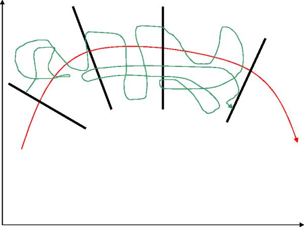
A schematic view of Milestoning. The red arrow is the reaction coordinate and in green we draw an exact reactive trajectory that is initiated at the reactants (R) and is terminate at the last interface (P). The interfaces are shown as thick black lines orthonormal to the reaction coordinate.

An ensemble of trajectories of this type provides the reaction rate as a function of time. For example, the number of molecules in the reactant state N_R (t) at time t is frequently modeled by an exponential decay as a function of time

$$N_R\left(t\right)=N_0\exp [-\lambda t]$$ (2)

The number of trajectories initiated in the reactant state is N₀ and λ is the apparent rate constant. The difficulty in estimating rate constants by straightforward simulations of individual trajectories and fitting the data against equation (2) is of cost. Because of limited computer power Molecular Dynamics trajectories are typically restricted to the sub-microsecond time scale. Ensemble of such trajectories would be (of course) significantly more costly. Milestoning makes it possible to compute the ensemble of reactive trajectories at a fraction of the cost, which in the present example is at least one thousand.

In Milestoning we assume that an equivalent representation of reactive trajectories can be assembled from short trajectories between Milestones (figure 2). Trajectories are renewed at the interfaces by sampling from a pre-determined stationary distribution at the interface. In the present manuscript we restrict our attention to conditions close to thermal (canonical) equilibrium. However, any known stationary distribution can be used, even far from equilibrium, as long as it represents a steady flux. The renewal is done with a fixed value of the reaction coordinate in the hypersurface orthonormal to the reaction coordinate at i and not necessarily at the point in which the trajectory we wish to renew was terminated. This loss of memory in the interface differentiates Milestoning from other Transition Path Sampling procedures (like TPS¹⁹, TIS²⁰, and Forward Flux²² that continue the terminated trajectory from the same point in which it was stopped). The spatial memory loss of Milestoning can be made exact with a special choice of the reaction coordinate and the dynamics³⁵. However, in general it is an approximation. The approximate re-sampling at the interface overcomes a significant statistical problem (getting a statistically meaningful number of trajectories to terminate at a particular interface). It allows us to push the time scales that we can study with Molecular Dynamics significantly further than is possible with other algorithms. It also allows us to investigate processes that do not follow exponential kinetics and mix diffusion and hopping over barriers. Below we consider in more details the approximations made in Milestoning and then we discuss why the calculations are significantly more efficient.

Figure 2.

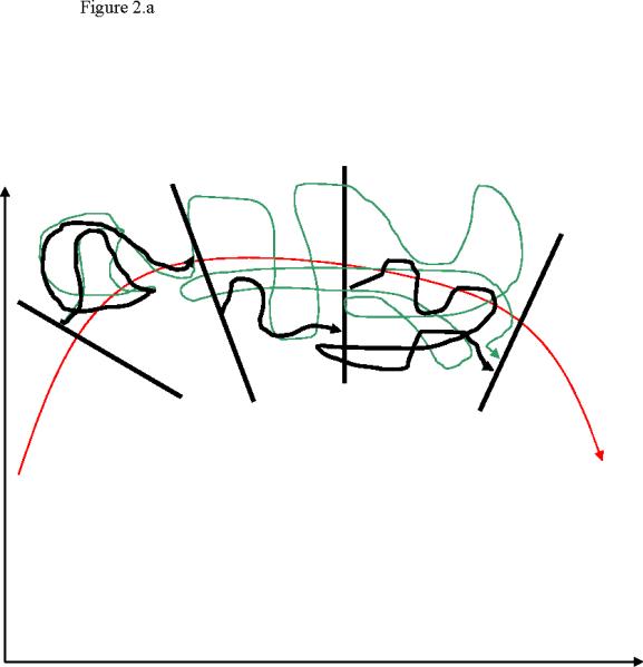
A schematic picture of the Milestoning approximation. A complete exact trajectory is shown in green as in Figure 1. Also shown are fragments of a trajectory in black (2.a). There are three trajectories fragments that we “glue”. The assumption is that the relaxation times in the hyperplane perpendicular to the reaction coordinate are short. Therefore we can sample from equilibrium at the interface and the short relaxation times at the interface (compared to the transition time between the Milestones) can be ignored. Since we have an ensemble of trajectories it should not matter (provided that our assumption is correct) where we initiate the trajectory at the interface. Also shown in blue lines (2.b) the probability densities of terminating trajectories at the Milestones. If we know the probability densities of the terminating trajectories we can sample the fragmented trajectories directly from these distributions. In previous²³,³³,³⁴ and current applications of Milestoning we assume that equilibrium densities can approximate the terminating distributions. A distribution that provide an exact first passage time is found in ³⁵ and a new intriguing numerical protocol to sample these distributions was proposed in⁴⁸

There are two ways of thinking about the above approximation (figure 2). The first considers a single trajectory. If the time of relaxation to equilibrium within the hyperplane perpendicular to the reaction coordinate is much shorter than the transition time between the Milestones, then the relaxation time within the plane can be ignored. The total reaction time is just the sum of transition times between the Milestones. This view suggests a clear way to test the Milestoning approximation and to improve it. Since we are working with a finite number of interfaces, increasing the distance between the interfaces will better satisfy the separation of time scale (the time scale for the relaxation within the interface remains the same while the time scale for the transition between the interfaces is getting longer as we increase the separation). However, the computational efficiency of Milestoning decreases with a decrease in the number of interfaces. So a compromise between accuracy and efficiency should be made.

The second view, which is subtler and discussed extensively in³⁵, is based on the time evolution of the probability density. Instead of the motion of one trajectory at a time we consider the time evolution of an ensemble of trajectories. Let the probability density of trajectories that terminate in the hyperplane perpendicular to Milestone i be ρ_i (Γ), where Γ denotes the orthogonal hypersurface. This probability density is our best (exact) choice for renewing the trajectories at i. Unfortunately, this probability density is not known exactly except in special cases³⁵. The probability density is therefore approximated by an analytical function or using a simulation. An analytical approximation we have used in the past is that of an equilibrium distribution^33,34. Of course the terminating trajectories generate samples of the exact distributions at the nearby interfaces and the approximate form of the density can be tested for consistency. A computational technique that directly generates these distributions, and is still significantly more efficient than straightforward Molecular Dynamics, was proposed recently⁴⁸ and is a very promising direction.

We define the mean first passage time (MFPT) 〈t〉 as the time averaged over an ensemble of trajectories that are initiated at the reactants (Milestone 1) and terminated at the products (Milestone N). The last Milestone (products) is absorbing. The MFPT captures characteristics of the time evolution of the process. For example if the reactant population, N_R (t), decays exponentially as a function of time -- N_R (t) = N₀ exp(-λt) then the rate constant λ is given by 1/〈t〉. To compute the overall MFPT we use the formula developed in³², which was illustrated in³³ and re-derived in³⁵. For completeness of this paper we define the relevant variables, explain how they are extracted from the simulation, and provide the final formula.

We define K_ij (τ) the probability density that a trajectory initiated at Milestone i at time τ' = 0 will transition to Milestone j at time τ' = τ. The time integral ${\int }_0^{\infty }{K}_{ij}\left(\tau \right)d\tau =p_{ij}$ is the transition probability from state i to state j. The sum over all final states is normalized ${\sum }_j{p}_{ij}=1$. The last (products) Milestone is absorbing and p_NN = 1. We also define the transition matrix:

$${\left[\mathbf{K}\left(\tau \right)\right]}_{ij}=\left\{\begin{array}{cc}\hfill K_{ij}\left(\tau \right)\hfill & \hfill i\ne j\hfill \\ \hfill 0\hfill & \hfill \text{otherwise}\hfill \end{array}\right\}$$ (3)

The mean first passage time is then given by

$$\langle t\rangle =1^t\cdot {\int }_0^{\infty }\tau \mathbf{K}\left(\tau \right)d\tau \cdot {\left[\mathbf{I}-{\int }_0^{\infty }\mathbf{K}\left(\tau \right)d\tau \right]}^{-1}\cdot {\mathbf{Q}}_i$$ (4)

The symbols 1^t, I, and Q_i are a vector of all ones (1,1,…,1), the identity matrix, and a projection vector onto the initial Milestone (1,0,…0)^t respectively. From equation (3) it is obvious that the transition matrix K plays a dominant role in determining the kinetics of the system. Indeed in our previous papers on Milestoning and in the present study we estimate this matrix numerically by sampling. We initiate trajectories at each Milestone i according to Boltzmann distribution, constrained to the hypersurface at i, ρ_i (Γ)

$$\begin{array}{cc}\hfill & {\rho }_i\left(\Gamma \right)d\Gamma =Z^{-1}\delta (q-q_i)\exp [-\beta U\left(X\right)]d\Gamma \hfill \\ \hfill & Z=\int dX\exp [-\beta U\left(X\right)]\hfill \end{array}$$ (5)

We denote the reaction coordinate by q, the complete coordinate space by X, and the complementary space to q by Γ. We record the termination times of the trajectories at Milestone j. The number of termination events from Milestone i to j, L (i → j;τ, τ + Δτ), is counted during the time interval [τ, τ + Δτ]. We divide L (i → j;τ, τ + Δτ) by the total number of trajectories initiated at i, L_i, to estimate K_ij (τ)Δτ with the proper normalization.

$$K_{ij}\left(\tau \right)\Delta \tau \cong \frac{L(i\to j;\tau ,\tau +\Delta \tau )}{L_i}$$ (6)

Since all trajectories initiated at i terminate in the limit of long time we also have $L_i\equiv {\sum }_{j,k=1,\dots ,\infty }L(i\to j;k\cdot \Delta \tau )\cdot \Delta \tau$.

Estimating the elements of the transition matrix and their time dependence is necessary if the complete time evolution of the system is of interest (e.g. compute N_R (t) for a general, not necessarily exponential process). The theory and some examples of these general processes is discussed in detail in³³. The essence is a numerical solution of an integral equation for the probability of being at Milestone i in time t. These general calculations can be expensive since they require significant sampling of the three dimensional tensor K_ij (τ)(including the time “dimension).

On the other hand Equation (4) that provides the overall mean first passage time includes only integrals of the probability density, K_ij (τ), that are easier to estimate and require significantly less statistics. We have estimated the mean first passage time (MFPT) in the study of the allosteric transition of scapharca hemoglobin³⁴ using a relatively small number of trajectories. We focus on the MFPT also in the present study of folding/unfolding of a helical peptide.

So far we discuss the theory and the implementation of Milestoning. However, we did not discuss why Milestoning is beneficial to straightforward Molecular Dynamics. In³³ it was argued that the computational gain of using Milestoning compared to straightforward Molecular Dynamics is proportional to the number of Milestones if the process is diffusive and is exponential in the number of Milestones for activated transitions (states separated by a significant free energy barrier). For the completeness of this paper we repeat the qualitative arguments below. We also illustrate (as part of this manuscript) that the Milestoning calculations of helix folding is more efficient than straightforward Molecular Dynamics by a factor of thousands, enabling meaningful calculation of rates in complex systems.

Consider first a diffusive process along a (one dimensional) reaction coordinate. If the diffusion is on a “flat” energy surface (we shall consider the other limit next) then the time t it diffuses along a path length Y would be proportional to Y² (from the relationship - Dt : Y² where D is the diffusion constant). In Milestoning we consider diffusion between the M interfaces. Each pair is roughly separated by Y/(M - 1)≈ Y/M distance. The time of transition between two interfaces is therefore proportional to (Y/M)². The total time of a transition between M interfaces is M ·(Y/M)² = Y²/M. The computational time to observe a transition in Milestoning is therefore a factor of M shorter than a straightforward trajectory. We typically use close to one hundred Milestones so the computational gain is substantial. Consider next a significant barrier separating the two minima. If the system is close to thermal equilibrium, then the probability of making it to the top of the barrier is proportional to exp[-βΔU] where β is the inverse temperature and ΔU the barrier height with respect to the reactants. However if we divide the reaction path from the reactants to the top of barrier to M milestones then the probability of reaching the next Milestone is about exp[-βΔU / M]. Since we initiate the trajectories at a Milestone, the computational cost of computing the corresponding ensembles is proportional to a sum (instead of the product we have in MD)

$$\begin{array}{cc}\hfill & COST\left(Milestoning\right)\propto \sum _{i=1,\dots ,M}\exp [\beta \Delta U∕M]\hfill \\ \hfill & COST\left(MD\right)\propto \exp \left[\beta \Delta U\right]=\prod _{i=1,\dots ,M}\exp [\beta \Delta U∕M]\hfill \end{array}$$ (7)

For a typical number of Milestones (about one hundred), the gain can be staggering.

III. Computational protocol

Selection of initial seeds for the reaction coordinates

The use of a sample of SDP pathways that we propose in the present manuscript allows us to test concrete mechanisms, test their consistency with experimental data, and learn about characteristics of the transition. The guiding trajectories for helix unfolding pathways were generated using previous replica-exchange molecular dynamics simulations (REMD) of the blocked WH21 peptide¹⁴ (sequence WA₃HA₃RA₄RA₄RA₂). Both the N terminal and C terminal are uncharged. The N terminal is capped with CO-CH₃ group while the C terminal is terminated with NH₂ group. The simulations used 8 replicas with temperatures spanning 280-450 K and a Generalized Born/Surface Area (GB/SA) continuum solvation model and the CHARMM program (charm: ref 15). In a 30-ns long REMD trajectory starting from an α-helical structure, conformational equilibrium was reached after 15 ns. For the unfolding transition this simulation predicted a melting temperature T_m of 330-350 K, unfolding enthalpy ΔH = -10 kcal/mol and entropy of ΔS = -30 cal/(mol K). These values were in reasonable agreement with the experimentally observed values of T_m =296 K, ΔH = -12 kcal/mol and entropy of ΔS = -40 cal/(mol K)¹⁴. Our second REMD simulation was 15 ns in length and started from the extended structure. In this case the helical conformation was first attained after ca. 2.8 ns and equilibrium was reached after 10 ns.

We generated three helix-coil transition paths from the structures sampled in the GB/SA REMD simulations. For path 1 we employed the sample of 37,500 structures from the 367 K replica in the 30 ns (“equilibrium”) simulation, classified by the root-mean-square deviations (RMSD) of backbone atoms from an ideal helix and the number of α-helical hydrogen bonds (NAHB) for each structure. The subset with NAHB=8 was hierarchically clustered based on backbone RMSD using the MMTSB tool set⁴⁹. The path was initiated by selecting a random structure from the largest cluster, and a series of intermediates was then identified by analysis of pairwise RMSD and NAHB, producing a chain of 16 structures spanning the range of NAHB=17 (corresponding to the α-helix) to NAHB=0 (fully unfolded state). For the second path, we selected three structures from the 298 K replica of the 30 ns “equilibrium” REMD - one corresponding to the α-helix (NAHB=17), the second to unfolded C-terminal portion of WH21 (with NAHB=8 and hydrogen bonds formed in N-terminus only) and the third to the coil state (NAHB=0). The third path was constructed from the first 2.8 ns of the 298 K replica of the 15 ns (“folding”) simulation in which the helix is formed from an extended conformation. In this case we again used RMSD and NAHB analysis to find 15 structures spanning from NAHB=17 to NAHB=0.

In our analysis we did not count the hydrogen bonds of the blocking groups. The backbone RMSD between the nearest neighbors in the chains varied from 0.7 A to 2.5 A. The paths selected were arbitrary, in the sense that they do not correspond to any directly simulated transitions, but represent roughly random walks through configuration space constrained to follow a roughly sequential, or zipper, hydrogen bond breaking/formation mechanism with limited RMSD changes between neighbors. We chose the generation methods to make the paths as different as possible. Thus, for path 1 the initial structures were sampled from above the simulated T_m, where the population of partially unfolded intermediates is higher than at 298 K, and the path was required to pass through the most highly populated NAHB=8 intermediate. Path 2 was based on the same REMD simulation, but only three structures from the 298 K replica were employed in the initiation, and the intermediate was arbitrarily selected to correspond to the unfolded C-terminal of WH21. Finally, path 3 was initiated based on the structures sampled in the 298 K replica of the “folding” simulation, using that part of the trajectory in which the system first converts from coil to helix in the course of the random walk generated by the combined MD and MC that are part of the REMD algorithm.

In the next stage of path generation, the initial chains underwent iterative interpolation and optimization using the SDP algorithm, producing paths with: 77 milestones for path 1, 129 milestones for path 2 and 113 milestones for path 3. These paths are complete in the sense that they start at the folded (helix) state and end at unstructured (zero hydrogen bonds) conformation. The number of alternative paths grows very rapidly as a function of distance from the folded state. Therefore time scales calculated along one-dimensional paths are likely to be overestimated, since transition to the unfolded state is made to any of many unstructured conformations. Therefore most of the detailed analysis presented in the Results section is done on the path in the neighborhood of the helix. There the number of alternative paths is smaller and time scale estimates is more likely to be meaningful.

Path calculations

Optimization of the initial guesses for intermediate structures along the paths follows. To speed up convergence the minimum energy paths were computed in two steps. The structures along the guess path were fed first to the SPW (Self Penalty Walk) algorithm⁴³ (module chmin in MOIL⁴⁷ and https://wiki.ices.utexas.edu/clsb/wiki). The optimized paths are computed with the discrete representation of a line integral with equi-distance restraints introduced by Elber and Karplus⁵⁰ and further refined by Czerminski and Elber⁵¹. This type of restraints was adopted by the NEB⁴⁵ and by the Maxflux⁴⁰ algorithms for calculations of reaction coordinates. In brief, the line integral is approximated by a finite difference expression

$$\begin{array}{c}S\left[X\left(l\right)\right]={\int }_{X_R}^{X_L}G\left(X\left(l\right)\right)\cdot dl\cong \sum _{i=1}^{N-1}G\left(X\left(l_i\right)\right)\Delta l_{i,i+1}+\hfill \\ \hfill +\sum _i\lambda {(\Delta l_{i,i+1}-\langle \Delta l_{i,i+1}\rangle )}^2+\sum _i\rho \exp \left[-\frac{\kappa \Delta l_{i,i+2}^2}{{\langle \Delta l_{i,i+2}\rangle }^2}\right]+E.C.\end{array}$$ (8)

In the context of the present manuscript the integrand G(X(l)) can be either U(X)/L in the SPW algorithm⁵¹ (L is the path length) or $\sqrt{\nabla U^t\nabla U}$ in the calculations of the SDP³⁹. The discrete length element is given by $\Delta l_{i,i+1}=\sqrt{{(X_{i+1,s}-X_{i,s})}^t(X_{i+1.s}-X_{i,s})}$. The path constraints apply to only a subset of the coordinates that are the Cartesian positions of the C_α atoms of the peptide. This subset is denoted by the index “s” in the above formula for the distance Δl_i,i+1. The parameter λ restrains all length elements to be similar to the average 〈Δl_i,i+1〉, and the term with the next nearest neighbor distance (Δl_i,i+2) reduces the path curvature. The restraint on next nearest neighbor distance was not used in the SDP calculations. The last terms (E.C.) are the Eckart Conditions expressed as six linear constraints³³ (three on translation and three on overall rotations). The path is optimized with a conjugate gradient minimizer or simulated annealing subject to the above linear constraints as a function of all the intermediate structures X_i.

Structures along the path were added between intermediate conformations to ensure that the difference between sequential structures did not exceed 0.6Å RMS after optimal overlap and optimization of the functional. The results of the SPW optimization were input to compute three different SDP paths with a discrete form of the functional of equation (8)³⁹. The optimizations are assumed converged when no significant changes in the structures are observed with more optimization cycles.

The paths are computed using the package MOIL with the Generalized Born model for solvation⁵², but are otherwise in vacuum. Water molecules are not included in the calculation of the SDP since the flat energy surface for solvent molecules and their permutations suggest low energy barriers and high degeneracy for their motions. Floppy solvent structure at room temperature does not support the use of a minimum-energy-path model and the generalized Born model mimics a potential of mean force more appropriate in the present context. Explicit solvation is (of course) included in the calculations of the short-time Milestoning trajectories.

Milestoning calculations

To compute short terminating trajectories between Milestones we follow two steps: (i) sample configurations in the Milestones to generate initial stationary distribution at the interfaces, and (ii) integrate trajectories initiated from the sample of step (i) and Maxwell velocity distribution until the trajectories terminate on nearby Milestones. Once a set of terminating trajectories and their corresponding time lengths are recorded we use equation (4) to estimate the overall first passage time of the early events of the folding/unfolding transition of the peptide.

In preparation for step (i) we solvate the peptide in a cubic box of water of 41.8³Å³ with periodic boundary conditions for each peptide configuration, q(l_i), along the SDP. The water model is TIP3P⁵³ (the geometry of the water molecules is fixed with the matrix-SHAKE algorithm^54,55). The force field is united atom OPLS⁵⁶ as implemented in our code MOIL⁴⁷. Four chloride ions were added to ensure electric neutrality and Particle Meshed Ewald⁵⁷ was used to sum electrostatic interactions. The Lennard Jones interactions were truncated at 8Å and the time step was 0.5 femtosecond (fs). We first equilibrate the solvent for 20 picoseconds around the frozen configurations of the peptide (from the SDP calculations). The system is coupled to a heat bath by velocity scaling in the first 20 ps (velocity scaling or the iso-kinetic ensemble ensures canonical ensemble of configurations⁵⁸). The remaining 20 picoseconds were run in the NVE ensemble. The system is sufficiently large so that the differences between an assigned temperature and computed temperature from the average kinetic energy are small. The standard deviations of the temperatures in the NVE ensembles along the paths are less than 10 degrees. The last coordinate sets of the trajectories of solvent (+ frozen peptide) are saved and used as starting points for simulations to generate the stationary distributions at the interface

The NVE simulations in the hyperplanes orthogonal to the reaction coordinate are ordinary Molecular Dynamics simulations of the peptide and solvent supplemented by linear constraints³³. The simulation parameters are the same as in the previous simulations equilibrating the solvent except that now the peptide is allowed to move. The MD trajectories remain in the designed Milestone through application of the constraint

$$(X_s-q_{si})\cdot e_{si}=0e_{si}\cong \frac{q_{si+1}-q_{si-1}}{\mid q_{si+1}-q_{si-1}\mid }$$ (9)

The constraint is enforced with Lagrange's multiplier (appendix of ref 33). The coordinate vector of the system is X and its projection onto the subset of the selected variables (the Cartesian positions of the C_α atoms) is X_s. The unit vector e_si is normal to the hyperplane i along the reaction coordinate. The normal (which is e_si) and a point in the hyperplane (which is q_si) determine the position of the interface uniquely. Since the constraint is expressed in Cartesian coordinate it is also necessary to fix the global orientation and position of the molecule. This is achieved by six (linear) constraints (derived from the Eckart conditions) in addition to the path constraints above. This is similar to the discrete path calculations discussed in equation (8) and discussed in detail in³³. The simulations were run in the NVE ensemble for 50 picoseconds (ps) for each location along the reaction coordinate and structures were saved every 0.5ps. For each q_si we therefore have a sample of 100 conformations that are used to initiate the terminating trajectories between the Milestones.

In the second phase we compute Molecular Dynamics trajectories without the hyperplane constraint (equation (9)) while retaining the six constraints on overall molecular orientations. We keep the six constraints to enable convenient determination of termination times. Trajectories that are initiated at q_si are stopped and their times are recorded when (X_s - q_si-1) ·e_si-1 = 0 (termination at the previous milestone) or when (X_s -q_si+1)· e_si+1 = 0 (termination at the next milestone). Since the vectors q_sj and e_sj are expressed in Cartesian coordinates which are sensitive to overall molecular motions it is useful to constrain the C_α to a fixed overall orientation. The constraints used in phase (ii) are softer than the constraints used in the sampling phase and therefore a larger time step (1 fs) is used without significant loss of accuracy. The rest of the simulation parameters are kept the same.

Typically trajectories are terminated after a few or tens of ps. However, in extreme cases tens of nanoseconds are observed as well. Nevertheless the trajectory times are much shorter than the computationally estimated time scale for folding or unfolding, which is in the microseconds (along one dimensional paths), illustrating that Milestoning is indeed a lot more efficient than straightforward Molecular Dynamics. For example the accumulated time of all trajectories of the Milestoning calculation of the first SDP is 68ns. The computed first passage time for the transition was 2 microseconds, significantly longer than the time that was required to compute it.

The actual number of Milestones that are finally used in the estimate of the overall mean first passage time may be smaller than the number of structures generated along the SDP. To improve the Milestoning approximation we make sure that the trajectories are not too short and memory lost between initiation of trajectory and its termination are indeed achieved³³. In practice we found that the loss of velocity correlation is usually sufficient to obtain accurate results for the mean first passage time. We further determine empirically that for aqueous peptide systems 400fs is usually enough to de-correlate the velocity along the direction parallel to the reaction coordinate. Therefore if we sample termination times shorter than 400 fs between sequential Milestones, we increase the separation between the milestones by taking one out. For example rather than computing termination between Milestones i,i i+1 we compute them between i,i i+2. This extra calculation is not expensive since the trajectories below 400fs are cheap to compute and add only little to the overall cost.

Results and Discussions

We consider the dynamics of helix unfolding along three reaction coordinates. In the first path (path 1) we consider unfolding initiated at the N terminal. In the second path (path 2) the unfolding is initiated at the C terminal, and in the third (path 3) the helix breaks in the middle creating two short helices in the first step. Snapshots along the paths are shown in figure 3. We consider in the text below the initiation of unfolding and the complete unfolding pathways.

Figure 3.

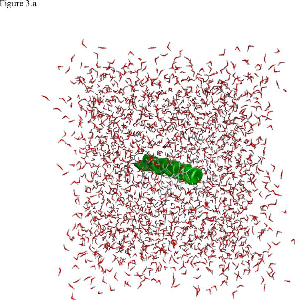
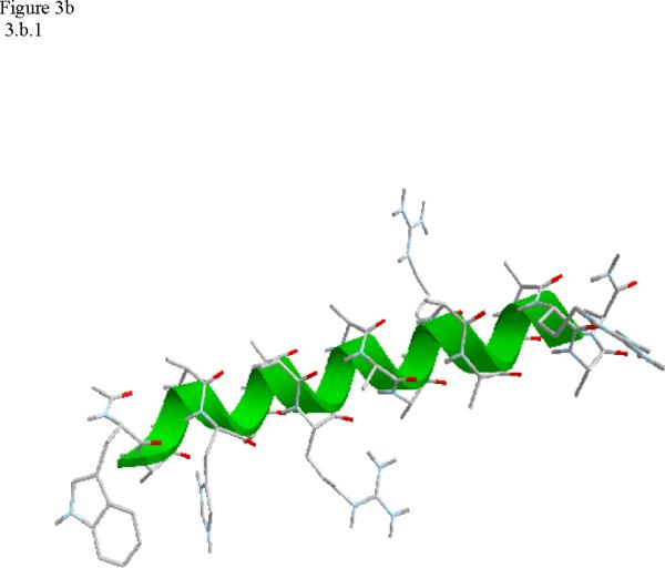
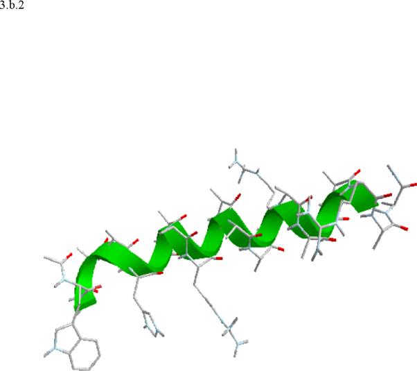
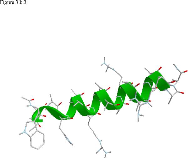
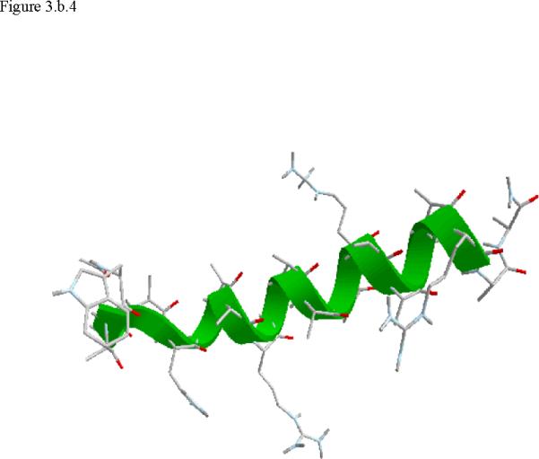
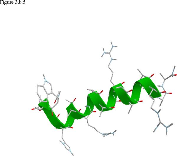
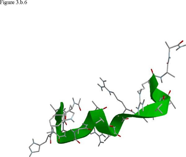
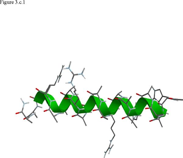
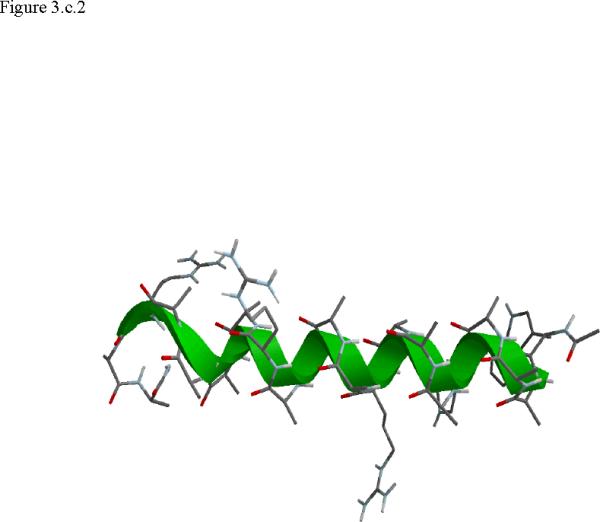
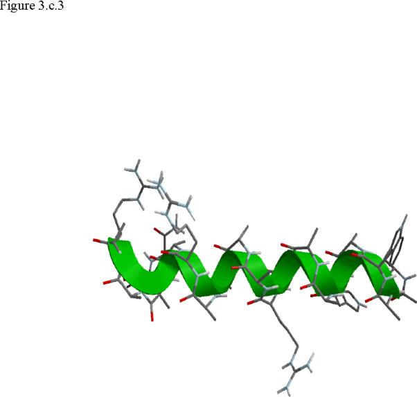
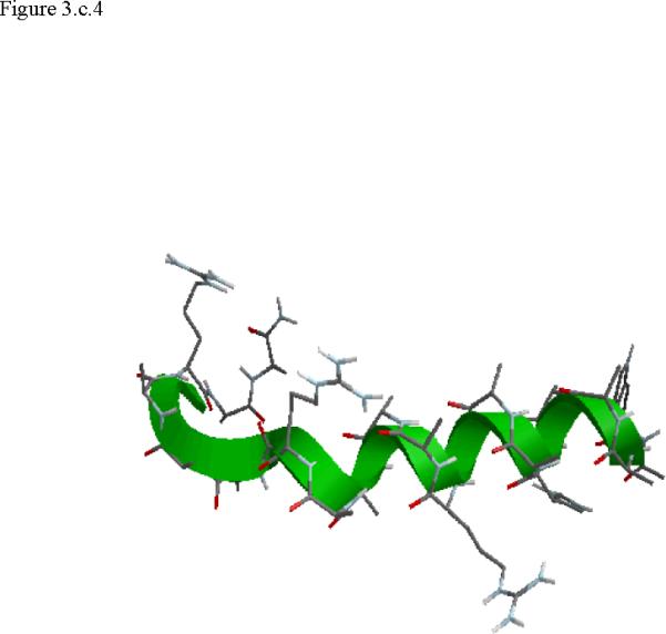
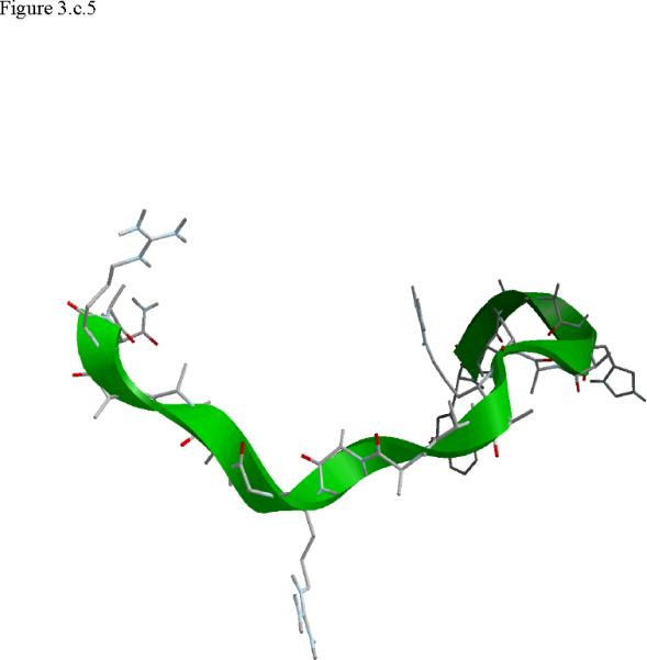
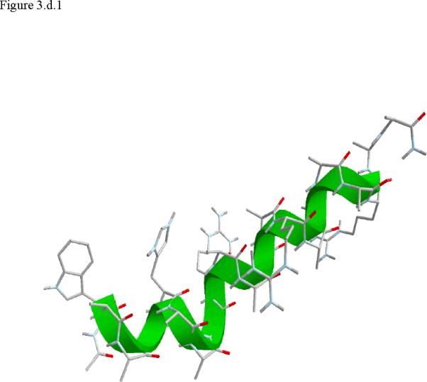
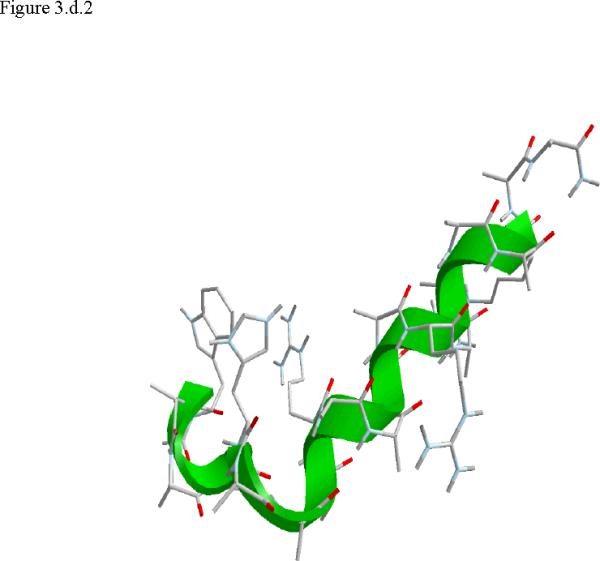
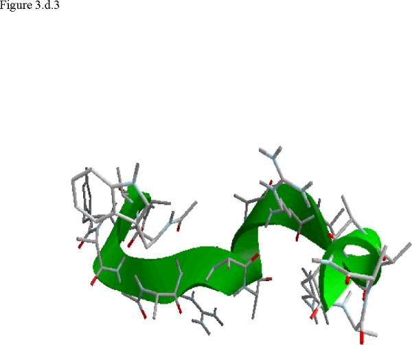
Structural snap shots along the three pathways. Ll the images displayed in the present manuscript were prepared with the cmoil/zmoil program, the graphic display module of MOIL⁴⁷ 3.a solvated structure of the helical conformation. For clarity the solvent was removed from all the structures that follow. Note also that in path 1 (figure 3.b) the N terminal is on the left wile in path 2 (figure 3.c) the C terminal is on the left. 3.b a sequence of peptide structures along the first path. 3.c second path. 3.d third path.

When does the first step of unfolding end? We have used quantitative and qualitative measures to define the end of the beginning. First we consider the reverse of the reactive flux in the Milestoning calculations. We seek the milestone i which is closest to the first milestone of the helical conformation such that the direction of the net flux of trajectories is reversed. Let n₊ be the number of trajectories that are terminating in the forward direction and n_- the number of trajectories terminated in the backward direction. We seek a pair of Milestone i and i +1 such that $(n_{+}^i-n_{-}^i)\cdot (n_{+}^{i+1}-n_{-}^{i+1})<0$. Near a stable conformation the flux of trajectories points to that state. A change in the direction of the net flux suggests a transition over a top of a free energy extremum. The net flux is estimated by the number of trajectories that terminate in the next Milestone minus the number of trajectories that terminate in the previous Milestone. In table 1 we list the number of trajectories between Milestones that led to our decision in paths 1-3. Second, we verify this choice by visual inspection, requiring significant structural changes in the subset of coordinates at q(l_i) where l_i is the index of the transition point. In retrospect the verification was not necessary since the flux condition works well. The “initiation” step of helix unfolding spans Milestones 1-14 in the first path, Milestones 1-58 in path 2, and Milestones 1-13 in the third path. In the analysis below we focus on path 1 that provide time scale consistent with experiment. The more significant barriers (and longer time scales) of paths 2 and 3 cannot be explained by a single dominant interactions and the excess energy (and free energy) is spread over many degrees of freedom.

Table 1.

The Number of trajectories initiated at a Milestone and terminating at (a) the milestone forward, (b) the milestone backward. The information was used to decide when the first barrier for unfolding was passed.

Path1	no. of traj. Forward/Total
Milestone before transition	44/100
Milestone after transition	74/100
Path 2
Milestone before transition	116/133
Milestone after transition	21/100
Path 3
Milestone before transition	34/100
Milestone after transition	61/100

Calculations of rate

The calculations of the complete unfolding rate along the three paths probe different processes compared to experiment. The calculations consider a transition from the helix into the neighborhood of only one unfolded conformation for each of the paths. The experiment considers a transition from the helix into any of the unfolded structures. The larger number of choices of alternative final conformations in the experiment makes it likely that the computation will provide a lower bound to the rate. We expect that simulated rates will be similar to experimental data if the final structure chosen in the calculations is one of highly preferred unfolded shapes, and that computed rates will be slower if multiple pathways to other unfolded structures contribute similarly to the rate. Indeed the mean first passage times that we obtain for one-dimensional unfolding (table 2) cover a diverse range of time scales, with the lowest values being comparable to the experimental rate. The relaxation rate is measured experimentally to be 3.3 × 10⁶ s^-1 at the 300 K^14,59. Nevertheless these estimates are still within typical errors that are seen with other studies. Errors in the force field can easily change the rates by a factor of 10. Consider an activated process that follows Arrhenius expression for the rate constant. Increasing of the barrier height by 1.5 kcal/mol at 300K, which is a typical error in condensed phase simulations, reduces the rate constant by a factor of 12. It is therefore unclear if the errors are a result of the assumed one-dimensional reaction coordinate, the force field, the Milestoning approximation, or other factors. The initiation of unfolding events that we examined and their corresponding rates provide some support to the force field we used. These rates are not in significant variance with those observed in straightforward multiple MD trajectories²⁷ suggesting that the results of our calculations are typical. We therefore continue to examine the mechanisms of unfolding along the paths.

Table 2. Mean first passage time.

The time scale for transitions from helical conformations, to the first step in unfolding and to the unfolded conformations. The times are given for the three paths that we considered.

	Unfolding time	Elementary step
Path 1	280ns	455ps
Path 2	7μs	1.58ns
Path 3	86μs	8.9ns

The kinetic of the first steps of unfolding (starting from the helix) are more likely to describe accurately experimental behavior when compared to the RP approach. Near the helix conformation the number of unfolding paths is small and parallel independent paths is a reasonable description of the process. In the discussion below we therefore focus on the early event, however we also analyze properties of the complete folding pathway as appropriate.

Efficiency of the calculations

In figure 4.a we show an example of a simulated first passage time distribution K_ij(τ) of transitions to two nearby Milestones. To differentiate between trajectories that terminate in the forward and the backward directions we use negative times to denote termination backward (on the previous Milestone). It is obvious that the time scale of termination at the nearby Milestones is significantly shorter than the time scale of the overall process (picoseconds versus microseconds). This illustrates the high efficiency of Milestoning. Even with 48 Milestones for the first path and one hundred trajectories launched from each Milestone (with a trajectory time of about 50ps, which is on the high side) the accumulated time to compute the rate is 100 × 48 × 50 ps = 240ns still significantly shorter that the time to compute a single trajectory probing the event. Note that for the calculations of the overall first passage time we need only the zero and the first moments of the above distribution. Therefore, despite the sparse sampling we are able to obtain results with acceptable (but significant) statistical error bars. For example halving the number of data points for the third unfolding path changes the time scale from 86µs to 205µs for the first 50 trajectories and to 79µs for the last 50 trajectories. If our estimates are accurate enough the time scales also suggest that the first path is significantly more likely from the kinetics viewpoint, even if thermodynamically configurations from all paths are observed in the Replica Exchange simulations.

Figure 4.

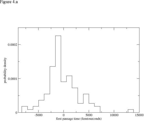
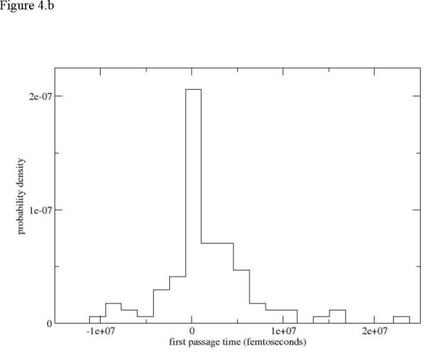
Local (between Milestones) first passage time distributions. 4.a Distribution sampled from Milestone 15 of the first path. Negative times denote termination of the trajectories on the previous Milestone and positive times termination in the forward direction. 4.b Distribution computed from the third path.

An extreme distribution of K_ij (τ) from path 3 is shown in figure 4.b. The trajectories are considerably longer since a smaller number of Milestones (29) was used along a less direct unfolding pathway compared to path 1. However a similar estimate to the one we did above suggests that Milestoning is still more efficient than straightforward MD. The maximum termination time is 22ns. A complete trajectory along all the 29 Milestones assuming the maximum time of transition for terminations at the Milestones (which is clearly an upper bound) requires 638ns. This is sill shorter by about a factor of 10 compared to the overall first passage time (eighty six microseconds) we estimated for this path (table 2).

Analyses of structural features of the transition

The analysis of the path includes changes in local variables such as specific torsion angles and global variables that capture the shape of the peptide, e.g. the radius of gyration. Besides the representation of distributions of relevant spatial variables, there is significant interest in their time dependence. In our analysis we wish to capture both, the spatial distributions of variables at a given instance of time and their time evolution. At each of the following figures we show several graphs that are color coded to indicate their position along the reaction coordinate. The black curve corresponds to the initial helical phase and the later time distributions are (in sequential order) red, green, blue and orange.

The radius of gyration

The complete path 1 is divided into five more-or-less equal segments. For example the initiation of unfolding in the first path includes 18 Milestones. The data presented in the graphs is collected from the conformational statistics generated from Milestones 1,5,10,15,18. In figure 5.a we show the variation in the radius of gyration of the C_α for several Milestones along the complete unfolding path (the C_α Cartesian coordinates define the space in which the reaction coordinate is optimized). The radius of gyration varies in value from about 7.5Å for the most compact conformations to 9.7 Å for the most extended structures. These are not very large deviations but they are nevertheless significant. The broadest distribution of radii of gyration is one step before complete unfolding (the blue curve) which is perhaps surprising. As we emphasized however, the RP approach does not measure correctly the diversity of structures of the unfolded state. This is since the sampling is performed in the neighborhood of particular structural images. The width of the last distribution in orange is therefore wider than the folded state but is not wider than the intermediate (blue) distribution.

Figure 5.

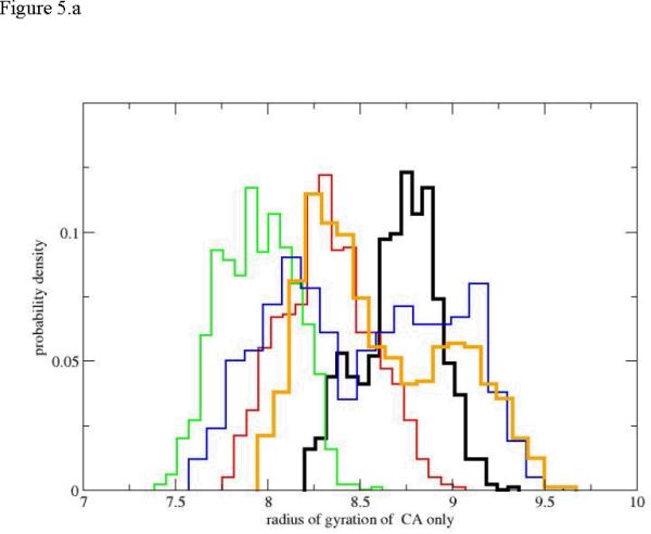
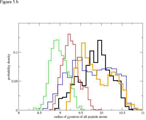
Probability density of the radius of gyration as a function of progress along the reaction coordinate for the first path. 5.a only C_α atoms are included in the calculation of the radius of gyration. 5.b all atoms are included. The black histogram is the distribution for the helical conformation. Red, green, blue and orange histograms follow sequentially the black curve along the path.

Another interesting observation is the non-monotonic behavior of the radius of gyration. The sequence of black, red, and green histograms clearly shows the average radius of gyration shrinking. Hence the backbone of the peptide (no side chains are considered) becomes more compact as unfolding is in progress. The red and green distributions are also not significantly broader than the distribution of the radii of gyration of the helix (first Milestone sampling). Only the blue and the orange distributions that lean towards the unfolded state show significant broadening compared to the initial helical state. In contrast to the red and green distributions they show an increase in the average value of the radius of gyration.

This observation also suggests that the use of radius of gyration as an order parameter to probe unfolding is problematic. The non-monotonic dependence of the radius of gyration on the RP makes it difficult to assign a position along the reaction coordinate given a value for a radius of gyration. The use of the radius of gyration as a reaction coordinate is therefore ambiguous. If we consider all the peptide atoms in figure 5.b (and not only the C_α) the evolution of the pathway shares similar properties to the backbone-only path. Not surprisingly the values of the radius of gyration are somewhat larger (the side chain atoms are now taken into account). However, we still observe the same qualitative trends of the compression of intermediate structures, and an increase in the average radius of gyration at late phases of the reaction (the blue and orange distributions). As before the blue and orange distributions are also considerably broader.

The analysis of the radius of gyration along the RP puts forward an interesting experimental suggestion. Since the radii of gyration (or the overall volume) of the folded and unfolded states are similar (black and orange distributions) we do not expect a significant change in the equilibrium constant relating the two states as a function of pressure. On the other hand the intermediate structures seem to have a smaller volume. Therefore the theoretical prediction is that pressure will reduce the time scale of the transition but will keep (more or less) the equilibrium constant of the folded and unfolded states intact.

Another widely used measure of size is the end-to-end distance computed from the nitrogen of the N terminal to the carbon of the carboxyl terminal. We show five histogram plots of the end-to-end distance distributions for path1 in figure 6. There is a clear and abrupt transition from a narrow distribution of distances at the helix conformation to a broad distribution of distances that consistently drift to more compact structures. The broad distributions overlap significantly and making it difficult to pinpoint a specific position along the reaction progress using the end-to-end distance. Interestingly the picture of the end-to-end distance is significantly different from what we have seen from the radius of gyration. A similar view is obtained also for the initiation of unfolding.

Figure 6.

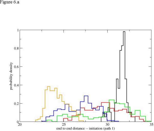
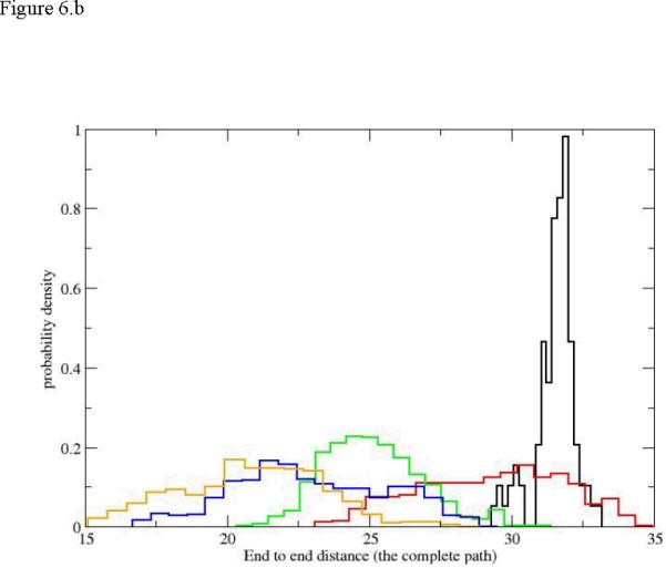
The probability density of the end-to-end distance as a function of the reaction coordinate. 6.a initiation of the unfolding pathway, 6.b the complete unfolding pathway of the first path (up to Milestone 18). The histograms and colors are the same as in figure 5.

The radius of gyration is a useful indicator of the compactness of the structure. However, other measures of shape can be useful. Honeycutt and Thirumalai⁶⁰ introduced two new shape measures constructed from the eigenevalues λ_i of the tensor of inertia (in addition to the radius of gyration). These measures were found useful in a number of studies of complex macromolecules⁶¹. The first is denoted by Δ and is defined by

$$\Delta =\frac{3}{2}\frac{\sum _{i=1,2,3}{({\lambda }_i-\stackrel{‒}{\lambda })}^2}{{\left(\sum _{i=1,2,3}{\lambda }_i\right)}^2}$$ (10)

The eigenvectors of the tensor of inertia are the λ_i. The average over the three eigenvalues is $\stackrel{‒}{\lambda }$. If the object is a sphere, all the eigenevalues are the same and Δ is zero, which is also its minimum. In figure 7 we show that the unfolding transition starts at reasonable high values of Δ and sequential distributions are shifted to lower values. The lower values indicate shapes that are more spherical than the initial (and also the final) state. Indeed the significant deviations from a spherical shape of the initial helix Milestone (the black histogram) and of the final unfolded Milestone (orange bins) are similar in size and distribution. For the initiation of the first path (figure 7b) we observe monotonic drift to more spherical shapes.

Figure 7.

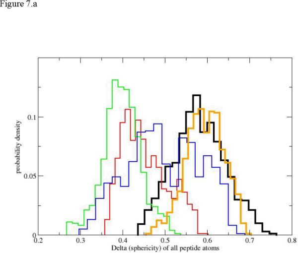
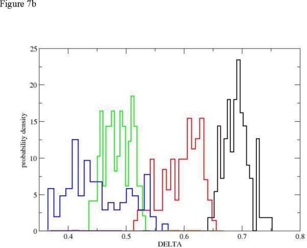
The probability density of the shape measure Δ for the first path. The histograms and colors are the same as in figure 5. 7.a: the complete path. 7.b: path initiation (up to Milestone 18, also only four distributions are used for clarity, no orange).

Another shape measure introduced by Honeycutt and Thirumalai is S

$$S=27\frac{\prod _{i=1,2,3}({\lambda }_i-\stackrel{‒}{\lambda })}{{\left(\sum {\lambda }_i\right)}^3}$$ (11)

In contrast to the Δ parameter S can be negative. For example if one (and only one) of the eigevalues is significantly smaller than the other two (and from the average). A “pita bread” shape will have a negative S. It is therefore of interest that our analysis never found negative S values suggesting a transition from cigar shapes to closely spherical conformations. In figure 8 we show that the changes (given only for the path initiation phase) clearly separate the states along the beginning of the unfolding pathway. The swollen configurations of the unfolded state were similar to the folded state using the measures of the radius of gyration and Δ. However, the last measure and the end-to end distance put the unfolded state in roughly the same domain as the intermediates.

Figure 8.

The probability density of the shape measure S for the initiation of the first path. The histograms and the colors are the same as in figure 5.

It is also intriguing to examine local torsions. Peptide conformations are usually determined by the value of the ψ dihedral angles. The variations in ω are negligible and the fluctuations in φ values are typically smaller than those of ψ. Even with the reduction in the number of relevant torsions there are still 21 ψ torsions in the peptide under consideration and we examined all of them. Detailing the fluctuations of all the twenty-one torsions in this manuscript can be exhausting and is not necessary. This is since these transitions tend to be local and we focus on the initial events of unfolding and the few active torsions. In figure 9a. we show the evolution of the distribution for the first torsion of interest ψ₁. The plot is surprising since the final distribution of the dihedral angle is concentrated near negative values of a helical conformation. Of course also the starting distribution is helical, making the unfolding process strongly non-monotonic (going from a helix to an extended chain and back to helix from the perspective of the first torsion). Only intermediate distributions (blue and red) “leak” to the extended chain but still maintain their hold in the helical configurations. The dihedral angle that does most of the work for initiation of the unfolding process is ψ₄. In figure 9b. we show a clear drift from a narrow distribution in the neighborhood of the helix, to a diffusive (red) distribution that covers most of the accessible torsion space, to different narrow distributions localized at the extended beta sheet configurations. Torsion angles of residue six and higher are unaffected by the unfolding of the edge of the helix (figure 9.c).). Similar localized transitions of dihedral angles assisted by large fluctuations of nearby torsions were found in other cases.

Figure 9.

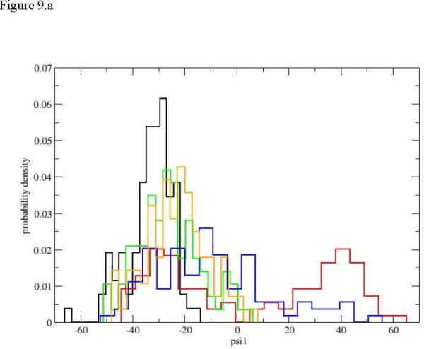
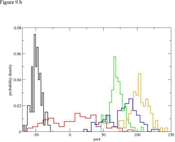
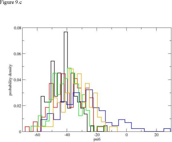
Probability densities for dihedral angle transitions along the first path. 9.a ψ₁, 9.b ψ₄, 9.c ψ₆. The histograms and colors are the same as in figure 5.

Concluding remarks

We have illustrated how the combination of reaction paths and Milestoning allow us to study at atomic detail the unfolding of a helical peptide. We are able to compute experimentally verifiable kinetics at long time scale that will be instrumental in calibrating and assessing force fields. An interesting observation that our analysis found is that the intermediate structures are more compact compared to the initial (folded) and the final (unfolded) states. This qualitative prediction of more compact transitional states suggests that the kinetic can be made faster if the pressure in the system increases. Increasing the pressure will not affect significantly the equilibrium between the folded and unfolded configurations. Three paths are considered N terminal, C terminal and unfolding from the middle. The significantly shorter time scale of the first path and the proximity of the time scale to the experimental unfolding rate suggest that the N terminal path is highly significant in accord with stochastic path calculations³¹. It will be of considerable interest to extend this study to a network of structural images representing Milestones between folded to unfolded configurations with time courses of transitions determined by first passage time distributions.

References

- (1).Brooks CL. Accounts Chem. Res. 2002;35:447. doi: 10.1021/ar0100172. [DOI] [PubMed] [Google Scholar]
- (2).Gnanakaran S, Nymeyer H, Portman J, Sanbonmatsu KY, Garcia AE. Current Opinion in Structural Biology. 2003;13:168. doi: 10.1016/s0959-440x(03)00040-x. [DOI] [PubMed] [Google Scholar]
- (3).Brooks CL. Current Opinion in Structural Biology. 1993;3:92. [Google Scholar]
- (4).Tobias DJ, Mertz JE, Brooks CL. Biochemistry. 1991;30:6054. doi: 10.1021/bi00238a032. [DOI] [PubMed] [Google Scholar]
- (5).Karpen ME, Tobias DJ, Brooks CL. Biochemistry. 1993;32:412. doi: 10.1021/bi00053a005. [DOI] [PubMed] [Google Scholar]
- (6).Mohanty D, Elber R, Thirumalai D, Beglov D, Roux B. Journal of Molecular Biology. 1997;272:423. doi: 10.1006/jmbi.1997.1246. [DOI] [PubMed] [Google Scholar]
- (7).Ferrara P, Apostolakis J, Caflisch A. Journal of Physical Chemistry B. 2000;104:5000. [Google Scholar]
- (8).Chowdhury S, Zhang W, Wu C, Xiong GM, Duan Y. Biopolymers. 2003;68:63. doi: 10.1002/bip.10216. [DOI] [PubMed] [Google Scholar]
- (9).Zhang W, Lei HX, Chowdhury S, Duan Y. Journal of Physical Chemistry B. 2004;108:7479. [Google Scholar]
- (10).Garcia AE, Sanbonmatsu KY. Proceedings of the National Academy of Sciences of the United States of America. 2002;99:2782. doi: 10.1073/pnas.042496899. [DOI] [PMC free article] [PubMed] [Google Scholar]
- (11).Garcia AE, Sanbonmatsu KY. Proteins-Structure Function and Genetics. 2001;42:345. doi: 10.1002/1097-0134(20010215)42:3<345::aid-prot50>3.0.co;2-h. [DOI] [PubMed] [Google Scholar]
- (12).Zhou RH, Berne BJ, Germain R. Proceedings of the National Academy of Sciences of the United States of America. 2001;98:14931. doi: 10.1073/pnas.201543998. [DOI] [PMC free article] [PubMed] [Google Scholar]
- (13).Simmerling C, Strockbine B, Roitberg AE. Journal of the American Chemical Society. 2002;124:11258. doi: 10.1021/ja0273851. [DOI] [PubMed] [Google Scholar]
- (14).Jas GS, Kuczera K. Biophysical Journal. 2004;87:3786. doi: 10.1529/biophysj.104.045419. [DOI] [PMC free article] [PubMed] [Google Scholar]
- (15).Brooks BR, Bruccoleri RE, Olafson BD, States DJ, Swaminathan S, Karplus M. J Comput Chem. 1983;4:187. [Google Scholar]
- (16).Sugita Y, Okamoto Y. Chemical Physics Letters. 1999;314:141. [Google Scholar]
- (17).Voter AF. Physical Review Letters. 1997;78:3908. [Google Scholar]
- (18).Hamelberg D, Mongan J, McCammon JA. Journal of Chemical Physics. 2004;120:11919. doi: 10.1063/1.1755656. [DOI] [PubMed] [Google Scholar]
- (19).Dellago C, Bolhuis PG, Geissler PL. Advances in Chemical Physics, Vol 123. Vol. 123. John Wiley & Sons Inc; New York: 2002. Transition path sampling; p. 1. [Google Scholar]
- (20).van Erp TS, Bolhuis PG. Journal of Computational Physics. 2005;205:157. [Google Scholar]
- (21).Moroni D, Bolhuis PG, van Erp TS. Journal of Chemical Physics. 2004;120:4055. doi: 10.1063/1.1644537. [DOI] [PubMed] [Google Scholar]
- (22).Allen RJ, Frenkel D, ten Wolde PR. Journal of Chemical Physics. 2006;124:17. doi: 10.1063/1.2140273. [DOI] [PubMed] [Google Scholar]
- (23).Faradjian AK, Elber R. Journal of Chemical Physics. 2004;120:10880. doi: 10.1063/1.1738640. [DOI] [PubMed] [Google Scholar]
- (24).Daura X, Gademann K, Schafer H, Jaun B, Seebach D, van Gunsteren WF. Journal of the American Chemical Society. 2001;123:2393. doi: 10.1021/ja003689g. [DOI] [PubMed] [Google Scholar]
- (25).Yeh IC, Hummer G. Journal of the American Chemical Society. 2002;124:6563. doi: 10.1021/ja025789n. [DOI] [PubMed] [Google Scholar]
- (26).Buchete NV, Hummer G. Journal of Physical Chemistry B. 2008;112:6057. doi: 10.1021/jp0761665. [DOI] [PubMed] [Google Scholar]
- (27).Sorin EJ, Pande VS. Biophysical Journal. 2005;88:2472. doi: 10.1529/biophysj.104.051938. [DOI] [PMC free article] [PubMed] [Google Scholar]
- (28).Czerminski R, Elber R. Journal of Chemical Physics. 1990;92:5580. [Google Scholar]
- (29).Czerminski R, Elber R. Proceedings of the National Academy of Sciences of the United States of America. 1989;86:6963. doi: 10.1073/pnas.86.18.6963. [DOI] [PMC free article] [PubMed] [Google Scholar]
- (30).Wales J, David . Energy Landscapes with applications to custers, biomolecules and glasses. Cambridge University Press; Cambridge: 2003. [Google Scholar]
- (31).Cardenas AE, Elber R. Biophysical Journal. 2003;85:2919. doi: 10.1016/S0006-3495(03)74713-4. [DOI] [PMC free article] [PubMed] [Google Scholar]
- (32).Shalloway D, Faradjian AK. Journal of Chemical Physics. 2006;124 doi: 10.1063/1.2161211. [DOI] [PubMed] [Google Scholar]
- (33).West AMA, Elber R, Shalloway D. Journal of Chemical Physics. 2007;126 doi: 10.1063/1.2716389. [DOI] [PubMed] [Google Scholar]
- (34).Elber R. Biophysical Journal. 2007;92:L85. doi: 10.1529/biophysj.106.101899. [DOI] [PMC free article] [PubMed] [Google Scholar]
- (35).Vanden Eijnden E, Venturoli M, Ciccotti G, Elber R. Journal of Chemical Physics. 2008;129:174102. doi: 10.1063/1.2996509. [DOI] [PMC free article] [PubMed] [Google Scholar]
- (36).Cardenas AE, Elber R. Proteins-Structure Function and Genetics. 2003;51:245. doi: 10.1002/prot.10349. [DOI] [PubMed] [Google Scholar]
- (37).Akiyama S, Takahashi S, Kimura T, Ishimori K, Morishima I, Nishikawa Y, Fujisawa T. Proceedings of the National Academy of Sciences of the United States of America. 2002;99:1329. doi: 10.1073/pnas.012458999. [DOI] [PMC free article] [PubMed] [Google Scholar]
- (38).Truhlar DG, Garrett BC, Klippenstein SJ. Journal of Physical Chemistry. 1996;100:12771. [Google Scholar]
- (39).Olender R, Elber R. Theochem-Journal of Molecular Structure. 1997;398:63. [Google Scholar]
- (40).Huo SH, Straub JE. Journal of Chemical Physics. 1997;107:5000. [Google Scholar]
- (41).Schlitter J, Engels M, Kruger P, Jacoby E, Wollmer A. Mol. Simul. 1993;10:291. [Google Scholar]
- (42).Cho SS, Levy Y, Wolynes PG. Proceedings of the National Academy of Sciences of the United States of America. 2006;103:586. doi: 10.1073/pnas.0509768103. [DOI] [PMC free article] [PubMed] [Google Scholar]
- (43).Nowak W, Czerminski R, Elber R. Journal of the American Chemical Society. 1991;113:5627. [Google Scholar]
- (44).Ulitsky A, Elber R. Journal of Chemical Physics. 1990;92:1510. [Google Scholar]
- (45).Jonsson H, Mills G, Jacobsen KW. Nudged elastic band method for finding minimum energy paths of transitions. In: Berne BJ, Ciccotti G, Coker DF, editors. Classical and quantum dynamics in condensed phase simulations. World Scientific; Singapore: 1998. p. 385. [Google Scholar]
- (46).E WN, Ren WQ, Vanden-Eijnden E. Phys. Rev. B. 2002;66:4. [Google Scholar]
- (47).Elber R, Roitberg A, Simmerling C, Goldstein R, Li HY, Verkhivker G, Keasar C, Zhang J, Ulitsky A. Computer Physics Communications. 1995;91:159. [Google Scholar]
- (48).Vanden-Eijnden E, Venturoli M. submitted. 2008 [Google Scholar]
- (49).Feig M, Karanicolas J, Brooks CL. MMTSB Tool Set. The Scripps Research Institute; La Jolla, CA: 2001. [Google Scholar]
- (50).Elber R, Karplus M. Chemical Physics Letters. 1987;139:375. [Google Scholar]
- (51).Czerminski R, Elber R. International Journal of Quantum Chemistry. 1990;167 [Google Scholar]
- (52).Onufriev A, Bashford D, Case DA. Proteins-Structure Function and Bioinformatics. 2004;55:383. doi: 10.1002/prot.20033. [DOI] [PubMed] [Google Scholar]
- (53).Jorgensen WL, Chandrasekhar J, Madura JD, Impey RW, Klein ML. Journal of Chemical Physics. 1983;79:926. [Google Scholar]
- (54).Ryckaert JP, Ciccotti G, Berendsen HJC. Journal of Computational Physics. 1977;23:327. [Google Scholar]
- (55).Weinbach Y, Elber R. Journal of Computational Physics. 2005;209:193. [Google Scholar]
- (56).Jorgensen WL, Tiradorives J. Journal of the American Chemical Society. 1988;110:1657. doi: 10.1021/ja00214a001. [DOI] [PubMed] [Google Scholar]
- (57).Essmann U, Perera L, Berkowitz ML, Darden T, Lee H, Pedersen LG. Journal of Chemical Physics. 1995;103:8577. [Google Scholar]
- (58).Abrams JB, Tuckrman ME, Martyna G,J. Computer simulations in condensed matter: From materials to chemical biology. Vol 1. Vol. 1. Springer; Berin: 2006. [Google Scholar]
- (59).Jas GS, Eaton WA, Hofrichter J. Journal of Physical Chemistry B. 2001;105:261. [Google Scholar]
- (60).Honeycutt JD, Thirumalai D. Journal of Chemical Physics. 1989;90:4542. [Google Scholar]
- (61).Dima RI, Thirumalai D. Journal of Physical Chemistry B. 2004;108:6564. [Google Scholar]