Abstract
Background and Aims
To model plasticity of plants in their environment, a new version of the functional–structural model GREENLAB has been developed with full interactions between architecture and functioning. Emergent properties of this model were revealed by simulations, in particular the automatic generation of rhythms in plant development. Such behaviour can be observed in natural phenomena such as the appearance of fruit (cucumber or capsicum plants, for example) or branch formation in trees.
Methods
In the model, a single variable, the source–sink ratio controls different events in plant architecture. In particular, the number of fruits and branch formation are determined as increasing functions of this ratio. For some sets of well-chosen parameters of the model, the dynamical evolution of the ratio during plant growth generates rhythms.
Key Results and Conclusions
Cyclic patterns in branch formation or fruit appearance emerge without being forced by the model. The model is based on the theory of discrete dynamical systems. The mathematical formalism helps us to explain rhythm generation and to control the behaviour of the system. Rhythms can appear during both the exponential and stabilized phases of growth, but the causes are different as shown by an analytical study of the system. Simulated plant behaviours are very close to those observed on real plants. With a small number of parameters, the model gives very interesting results from a qualitative point of view. It will soon be subjected to experimental data to estimate the model parameters.
Key words: Rhythms, plasticity, plant growth model, GREENLAB, interactions, branching system, fructification, emergent properties
INTRODUCTION
The architecture of a plant is the expression of equilibrium between endogenous processes and exogenous constraints exerted by the environment (Barthélémy and Caraglio, 2007). That is why all aspects of plant growth must be combined to build a reliable model. In this context, the coupling of morphological models with physiological ones gave birth to the so-called functional–structural models (Sievänen et al., 2000). They provide a sound basis for modelling the interrelations between physiological processes and morphological structures (Wernecke et al., 2006).
However, modelling of interactions between a plant and its environment remains a weak point in most models (Kurth, 1994; Le Roux et al., 2001). In addition to models of spatial interactions (Mech and Prusinkiewicz, 1996; Blaise et al., 1998), some models where architecture depends on functioning have been developed but they mostly concern the branching system (Borchert and Honda, 1984; Perttunen et al., 1996; Prusinkiewicz et al., 1997; Balandier et al., 2000). Nevertheless, plasticity in trees is not only visible at the level of the branching system but is a more general phenomenon, as shown by studies on the morphology of beech (Nicolini, 2000) or spruce trees (Deleuze, 1996). In this context, a new version of the GREENLAB model (Yan et al., 2004) was developed in Mathieu (2006) with full interactions between organogenesis and photosynthesis: the organogenetic rules of the plant are dynamically controlled by the available biomass. Among others, the numbers of fruits and branches are given by increasing functions of the ratio of available biomass to plant demand. This ratio is a variable representative of the balance between sources and sinks during plant growth and was called the rate of growth demand satisfaction in Drouet and Pagès (2003).
Simulations of plant growth with this model revealed periodic patterns in fruit or branch appearance for sets of well-chosen parameters. Such emergent properties can be explained by the underlying principles of the model: a high production of biomass induces a high rate of growth demand satisfaction and hence a large number of fruits. These numerous fruits attract biomass that will not be allocated to leaves, whose surface area might be (relatively) reduced. Thus biomass production, and consequently the rate of growth demand satisfaction, might decrease. In such a case, fewer fruits appear, more biomass is allocated to leaves, and so on. Rhythms are automatically generated.
Such a model is relevant for numerous real plants. In Wardlaw (1990), the author was interested in the growth of temperate fruit trees like apple trees and noticed that ‘heavy fruiting, which reduces shoot growth, will also reduce the formation of new flowers and results in poor fruit production in the following year’. In perennial plants, these phenomena of ‘mast seedings’, i.e. the succession of ‘high and low years in reproduction whereas environmental conditions are not bimodal’, are well known (Innes, 1993; Kelly and Sork, 2002). The proportional matter distribution between vegetative parts and fruits showed a cyclic pattern in cucumber plants (Marcelis, 1992) and a simulation model has been implemented (Marcelis, 1994). Similar studies were conducted on capsicum plants and these revealed a ‘linear relationship between abortion and the source–sink ratio’ (Marcelis et al., 2004; Heuvelink et al., 2006).
In the present model, the same mechanisms of balance between sources and sinks, combined with the influence of biomass acquisition on organogenesis, induce rhythms in branch formation. Such phenomena were observed in trees. For example, Lusk and Le-Quesne (2000) studied the periodicity of whorl formation in Araucaria araucana and suggested that this periodicity was probably linked to the whole-plant carbon balance. It seems that the plant needs to accumulate enough reserves to be able to initiate the construction of a new branch whorl.
The following is a brief presentation of the GREENLAB model and how interactions between organogenesis and photosynthesis are implemented, mainly concerning the branching system and regulation of fruiting. Model simulations showed the appearance of rhythms under given conditions. The model is based on the theory of discrete dynamical systems. The explicit formalization of this system in simple cases helps us to understand the different origins of observed cyclic patterns. Several examples are presented with plant behaviour depending on the parameters of the model. The emergence of rhythms is explained in detail.
MATERIALS AND METHODS
Presentation of the model
The GREENLAB model of plant growth that was derived from AMAP models is used here (de Reffye et al., 1997). A detailed presentation of this functional–structural model can be found in de Reffye and Hu (2003) and Yan et al. (2004). The mathematical framework of the model defined in de Reffye et al. (2003) and Cournède et al. (2006) allows an analytical study of the results and thus a better understanding of the system behaviour. In addition, it is possible to use optimization methods to calibrate the model. The plant is described as a dynamical system, and its growth is characterized by a time step, called the growth cycle, that depends on plant development. Its duration can vary from a few days for herbaceous plants to 1 year for trees of temperate regions.
Plant architecture can be seen as a hierarchical system in which the axes are grouped into categories called ‘physiological ages’ and defined by the combination of a set of morphological, anatomical or functional parameters (Barthélémy et al., 1997). The plant is described as a collection of elementary units of different physiological ages (Barthélémy, 1991). Their organization to form the whole plant structure follows the rules of organogenesis defined in de Reffye et al. (2003) for the GREENLAB model. The elementary unit used here is the metamer which is defined as an internode bearing lateral organs, i.e. leaves and potential fructiferous or axillary buds whose numbers are given as genetic data of the plant. Some of these buds give birth to either fruits or lateral axes, whereas others may not develop. The development of an axis results from the functioning of its terminal apex, as long as it is alive. It can be either continuous or rhythmic depending on the plant. The beginning of the growth cycle corresponds in the first case to the appearance of one metamer; this is how annual plants are treated. In the second case, it coincides with the blossoming of the bud: the set of preformed metamers appears quite simultaneously compared with the growth cycle duration and forms a growth unit. The metamers are ordered according to different botanic laws (Barthélémy and Caraglio, 2007) and their number is computed as a function of the rate of growth demand satisfaction. Polycyclism is not considered in this paper. Thus, after the appearance of cohorts of organs, the architecture does not change during the growth cycle.
Sources are the seed and the active leaves. Fresh biomass production is considered to be proportional to crop transpiration and, to simplify, respiration is implicitly taken into account in a global coefficient of light conversion efficiency (Le Roux et al., 2001). The following empirical equation of resource acquisition is implemented in GREENLAB:
 |
1 |
Sf,t is the total green leaf area of the plant at cycle t, B is the product of potential evapotranspiration and transpiration efficiency divided by an empirical resistance, and A is an empirical coefficient characteristic of the competition for light in the canopy. In this study, A is considered to be constant. However, some more complex models can be implemented in the same framework taking into account variations of A according to plant architecture (Cournède and de Reffye, 2006). All the empirical parameters can be estimated from experimental data with methods described in Guo et al. (2006).
In most cases, it can be shown that growth can be divided into two phases: an exponential phase when the leaf area is small and, following this initial phase, a phase of stabilization of production. Biomass production is indeed limited by the value B/A, but may never reach it. Depending on the values of the parameters, the sequence of biomass (Qt) may decrease to zero, which induces plant death.
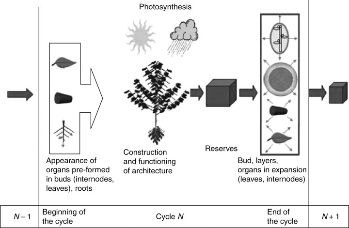
The matter produced by the plant is shared between existing and future organs according to a proportional allocation model (Warren-Wilson, 1972). Each organ o of chronological age d, i.e. present in the plant since d growth cycles, has a sink strength po(d) and receives at cycle t the fraction of biomass po(d)(Qt/Dt). The demand Dt is the sum of all the sink strengths of the plant, including organs (leaves, fruits and internodes) and rings resulting from the plant secondary growth and roots. The functioning of the plant during one growth cycle is described in Fig. 1.
Fig. 1.
Description of the GREENLAB growth cycle: blossoming of buds leads to appearance of organs in the plant. Each leaf is a source that produces biomass depending on the environmental conditions. It results in an incremental reserve pool available to all growing organs (leaves, internodes) and buds. The biomass allocated to buds is used for the construction of the preformed organs when they appear.
Interactions between organogenesis and photosynthesis
The biomass allocation system shows the importance of the ratio Qt/Dt, called the rate of growth demand satisfaction by Drouet and Pagès (2003). This ratio is a good measure of the competition between organs since available biomass is shared between all of them proportionally. A low ratio will correspond to strong competition, and vice versa. The present model uses it as the key variable to control plant plasticity. It monitors the main events in plant development at several levels – formation of branches, sizes of growth units and number of fruits (Mathieu, 2006) – and it can be used to modify some physiological characteristics along the growth. Thresholds are given as parameters of the model: when the rate of growth demand satisfaction exceeds these thresholds, additional organs are constructed.
At the beginning of growth cycle t, growth units appear on the plant with sizes proportional to the ratio Qt−1/Dt−1. On each of these growth units, a number of potential buds (given as an endogenous parameter of the plant) are formed. The ratio of available biomass to demand determines the number of these buds that will be activated to form new branches. Precisely, they will construct preformed organs for the first growth unit of the branch that will appear at the beginning of the next growth cycle (Mathieu et al., 2006b). Equation (2) gives bt,p, the number of buds activated in a growth unit of physiological age p:
 |
2 |
where the function |x| denotes the integer part of a real number x, and the function min(y, z) the smallest value between y and z. β1,p and βmax,p are, respectively, the minimum and maximum numbers of lateral branches born by a growth unit of physiological age p. More precisely, βmax,p is the number of potential buds of the growth unit. Lastly, 1/β2,p can be seen as the threshold for the formation of a new branch. According to the value of this threshold, different behaviours are observed. For a low value, the ramification can be continuous: the same number of new branches per growth unit appears at each growth cycle. An increase in the threshold value leads to sparser ramifications. Simulations of the model show that the ramification can become periodic.
Likewise, the dynamic evolution of the rate of growth demand satisfaction induces variations in fruit production through the growth cycles and even alternation between cycles of low and high fruit production. A threshold value slow is defined: fruits appear at cycle t + 1 if Qt/Dt > slow. Hence a sufficient value for the rate of growth demand satisfaction leads to fruit production. The fruit sinks will be competing with the leaf sinks, and those sources will receive less available biomass than previously. Consequently, the increase in demand and the decrease in biomass production due to smaller leaf areas will induce a lower value for the rate of growth demand satisfaction. If it goes under slow, fruit production will stop. More biomass will be allocated to leaves until the rate of growth demand satisfaction gets over the threshold, and so on.
The behaviour of the model has been tested first during the exponential phase of a Leeuwenberg model, where the number of branches may grow exponentially. Then, on plants for which the architectural rules limit the number of potential organs, the model behaviour has been studied for fruit production and branch appearance during the phase of stabilized production.
RESULTS
GREENLAB equations bring out the importance of the rate of growth demand satisfaction chosen to control different aspects of plant plasticity. The automatic generation of rhythms in branch and fruit formation is one of the emergent properties of this model. All simulations of the model shown in this paper were made using the Digiplante software developed at Ecole Centrale de Paris, France (Cournède et al., 2006). They correspond to purely theoretical studies; hence no unit is indicated on the graphs. For the sake of clarity, examples of trees with very simple topology are taken. For trees with complex topology (several orders of branching, numerous types of axes), simulated behaviours may be too intricate to study from a formal point of view. However, the results obtained fit in with observations made in nature.
Rhythms can be generated by two main causes in the model. First, if the plant topology is not limited, i.e. the number of organs can increase exponentially, a phenomenon of self-limitation may occur during the exponential phase of growth. Secondly, during the stabilization phase, if the topology is limited by botanical rules, the oscillations of the rate of growth demand satisfaction can be induced by the evolution of the demand. Examples of these two cases are presented in the following sections.
Plants in an exponential phase of growth
In this section are considered isolated plants or plants at the beginning of their growth, which corresponds to low values of ASf,t,t ∈ IN (see eqn 1). The example of a Leeuwenberg architectural model (Hallé et al., 1978) is taken for which the plant topology is not limited for the number of organs: the apical meristem dies after one growth cycle and the relay is taken by one or several lateral meristems. If there are at least two new branches on each metamer at each growth cycle, the development is exponential. In fact, this is not realistic and the branching system limits its development as observed, for example, by Borchert and Slade (1981). In the present model, it is supposed that the number of branches is controlled by the rate of growth demand satisfaction. According to model parameters, rhythms can be generated.
From eqn (1), the growth equations can be deduced in the particular case of the Leeuwenberg model, with all axes of same physiological age. It is supposed that leaves are sources and sinks during only one growth cycle. For the sake of simplicity, the secondary growth and the root system are not considered here (which is equivalent to a supposed constant proportion of biomass allocation to these compartments) but these hypotheses could be easily suppressed. pa and pe denote the leaf and internode sink strengths, respectively, ma, the number of leaves on a metamer, equal to the number of axillary buds, and e the leaf thickness. The bud sink strength pb is given by pb =mapa + pe. The amount of available biomass allocated to a bud is used for the construction of the corresponding growth unit. vt is the number of new growth units in the plant at cycle t, and bt the number of active buds on a metamer, determined by the equation
 |
As all the leaves are identical, we have
 |
3 |
The recurrent equation of the biomass production can be simplified:
It is noticed that biomass production is independent of plant topology. The behaviour of the recurrent sequence (Qt)t∈IN can be studied. The cycle p of the first double ramification is determined by solving
 |
Moreover, the function f is increasing and bounded; hence the sequence is monotonous and converges to the limit Q∞ that is the solution of the following equation:
 |
Two behaviours can be outlined according to the parameter values. If BC <1, the plant dies since the sequence (Qt)t∈IN converges to 0. Under this condition, leaf area is too small (high value for the thickness e or small leaf sink strength) to produce enough biomass in an environment which is not favourable (small value of B, the product of potential evapotranspiration and transpiration efficiency divided by an empirical resistance).
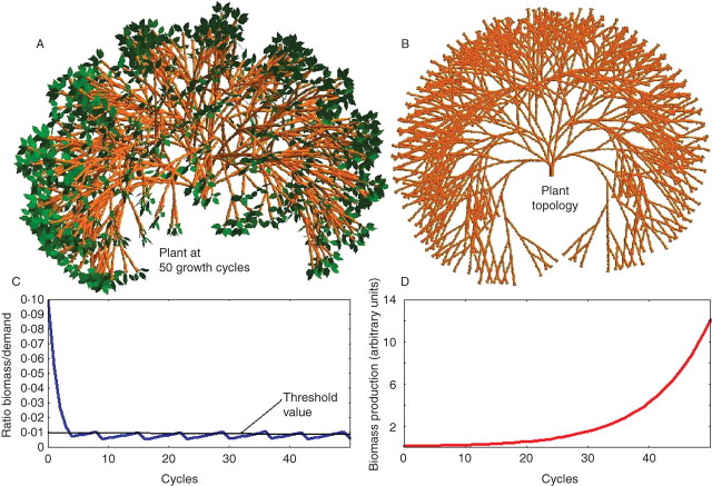
Otherwise, if BC >1, there is a strictly positive solution given in Grange (2006): AQ∞ = B + w(−CBe−CB) with w the Lambert function defined with w(x)ew(x) = x. It is noticed that the solution is inversely proportional to A, the parameter that quantifies the density. In this case, as long as biomass production is far below the limit value, the sequence (Qt)t∈IN increases rapidly, a new branch is formed when the rate of growth demand satisfaction exceeds the given threshold (see example in Fig. 2). Branch appearance entails an increase in demand and thus a decrease in the rate of growth demand satisfaction that may go below the threshold and thus inhibit new appearances of branches, until the biomass has increased enough so that the ratio of available biomass to demand may exceed the threshold, and so on. The rhythms observed only occur during the transitional phase. Indeed, after a while, the biomass production stabilizes, independently of the topology (see eqn 3). Therefore, as long as demand is low enough, the rate of growth demand satisfaction remains above the threshold. Consequently, the number of branches increases at each growth cycle and so does the demand. When this one is too high, the rate of growth demand satisfaction can no longer exceed the necessary threshold because biomass production is stable; at each growth cycle only one bud per metamer is activated, and the number of new organs stabilizes.
Fig. 2.
Appearance of rhythm in the branching system of a Leeuwenberg architectural model (Hallé et al., 1978). The plant (A) and its topology (B) are shown. On each metamer, two axillary buds are activated according to the rate of growth demand satisfaction. Parameters are A = 3·18 × 10−5, B = 0·11, C = 10. The simulation only presents the exponential phase of growth as shown by the graph of biomass production (D). The production limit is 674·04. It is observed that the ratio of available biomass to demand (C) has a periodic evolution: when it exceeds a threshold (with a value of 0·01), two branches are formed on each metamer, which multiplies the demand by two and decreases in proportion the rate of growth demand satisfaction (D).
Plant with stabilized production
After an exponential phase, the growth of plants slows down (high value of ASf,t, t ∈ IN in eqn 1). Rhythms can also be automatically generated in this case.
Fruit production
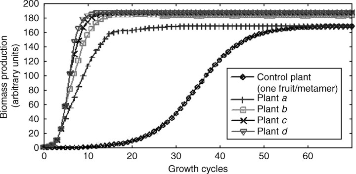
First, consider the example of a monocaulus plant with continuous growth – formation of one new metamer at each growth cycle. If the rate of growth demand satisfaction is high enough, i.e. Qt/Dt > slow, a fruit is created on this new metamer. According to the value of the threshold, several behaviours are underlined and can be related to observations on real plants (see Fig. 3B). After a transitional period of several growth cycles, the evolution of the rate of growth demand satisfaction becomes cyclic (Fig. 3A). Simulations show that the total biomass production at each growth cycle tends towards a limit that is lower for plants with the greater number of fruits (see Fig. 4). It is possible to optimize the threshold value to obtain the maximal fruit production (compromise between the number of fruits and their masses).
Fig. 3.
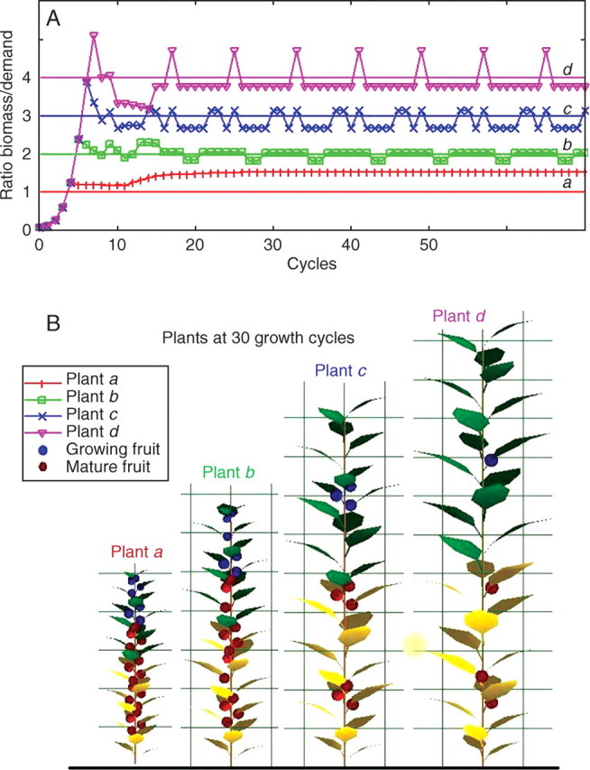
Influence of the threshold value of the rate of growth demand satisfaction for appearance of fruit. The behaviours of monocaulus plants are compared with the same entry parameters of the model (A = 3·53 × 10−4, B = 6·67 × 10−2, pe = 0·5, pa = 1, e = 0·025). But fruit appearance is more or less sensitive to the ratio of available biomass to demand. Plants a, b, c and d have, respectively, threshold values of 1, 2, 3 and 4. The lower the threshold is, the more fruits the plant produces and the smaller it is. It is observed that plant d grows much faster at the beginning, before the appearance of fruit. When fruits start to appear, the rate of growth demand satisfaction oscillates around the threshold (B), and rhythms in fructification are observed with different patterns for plants a, b, c and d (A).
Fig. 4.
Biomass production for monocaulus plants with fruit appearance depending on the rate of growth demand satisfaction. The behaviours of the monocaulus trees shown in Fig. 3 are compared. Plants a, b, c and d have, respectively, threshold values of 1, 2, 3 and 4. A control plant with a threshold value of 0 is added. It has the same limit behaviour as plant a (production of one new fruit at each growth cycle) but grows much slower at the beginning because it is influenced by early fruit appearance. In both cases, C = 38·2 can be computed, which gives Q∞ = 169·35. More generally, biomass production tends to stabilize, and it converges at 188·5 for plants c and d. Slight oscillations around the limit value for plant b are observed since the number of fruits in the plant is not constant.
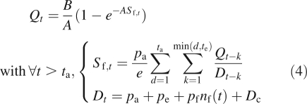
It is recalled that the leaf surface area is the result of successive increases during several growth cycles. The equation of biomass production (eqn 1) in this special case can be written as
 |
4 |
Note that po is the sink strength of an organ o (o is, respectively, a, e and f for leaves, internodes and fruits). The number of cycles during which the organs grow is tf for fruits and te for all other organs, and leaves remain active during ta growth cycles. The simplification is made that organ expansion is uniform, i.e. their sink strength is constant during their the whole of their growth. Dc is the demand for secondary growth, computed here with the pipe model theory (Shinozaki et al., 1964). The writing of the recurrent equations before fruit appearance, with distinction for t < ta, and t > ta (constant number of leaves), gives the evolution of biomass production and demand. It is thus possible to determine the first cycle at which a fruit appears, that is to say when the rate of growth demand satisfaction first reaches the threshold. After a given number of cycles, the number of active fruits at cycle t in the plant stabilizes if a dead fruit is immediately replaced by a new one. Then the plant demand is constant and the results given in Grange (2006) can be used to determine the limit of production: AQ∞ = B + w(−CBe−CB) with w the Lambert function. C depends on functional parameters (see Fig. 4) which among others is the one of the fruit sink variation function. The study of the dynamical system in the different cases allows the determination of the plant behaviour, like the number of consecutive growth cycles with fruit production.
Rhythms in branch appearance
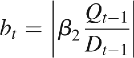
In this section are considered very simple ramified plants in their stabilization phase, with two physiological ages, one for the trunk and one for the branches. It corresponds to the Roux architectural model (Hallé et al., 1978) with no fruiting and a constant branch life span denoted t2. At cycle t, bt branches appear at the top of the trunk, depending on the rate of growth demand satisfaction:
 |
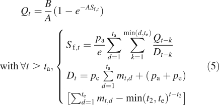
Equations of the model are quite similar to that of the monocaulus plant (eqn 4).
 |
5 |
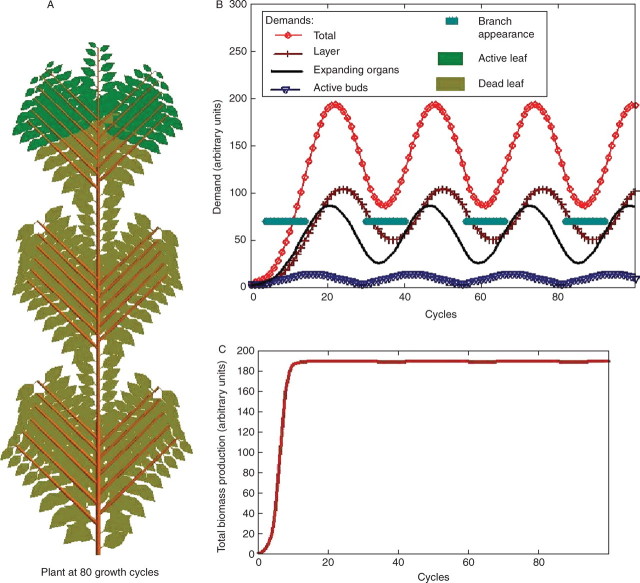
po, ta, tf and te have the same meanings as in eqn (4). mt,d is the number of metamers of chronological age d in the plant at cycle t. It is observed in Fig. 5C that the total biomass production increases exponentially at the beginning of growth. Then, it stabilizes and converges to the value Q∞ = B/A. Rhythms appear in branch formation owing to demand variations (Fig. 5D). As a matter of fact, the biomass production is quite low at the beginning; no branch is formed (small ratio of available biomass to demand). Then the ratio increases and new organs appear, entailing an increase in demand. If the demand increases too much, rhythms appear because the rate of growth demand satisfaction decreases under the necessary threshold. There will be no rhythm if the demand stabilizes at its maximum value Dmax such that β2Q∞ > Dmax, i.e. if the rate of growth demand satisfaction is always sufficient for the formation of t2 branches. In such a case, each dead branch is replaced by a new one. In the present example
| 6 |
Fig. 5.
Branched plant with branch appearance depending on the rate of growth demand satisfaction. Parameters are A = 3·53 × 10−4, B = 6·67 × 10−2, b2 = 1, pa = 1, pe = 0·5, pc = 1, ta = 15, te = 10 and branches remain alive for ten growth cycles. In (C), it is observed that the biomass production stabilizes (see eqn 1). The demand of the different organs varies according to their numbers (see B), leading to oscillations in the ratio of available biomass to demand and rhythm in branch formation (A). It is noticed that, except for the exponential phase, branches appear when demand is below a value depending on the threshold value of branch appearance (B) and biomass production tends to be 188·5 (C).
Complex rhythms with fruits and branches
The model can combine fruit and branch appearances that depend on the rate of growth demand satisfaction. More complex rhythms are then generated, according to plant parameters.
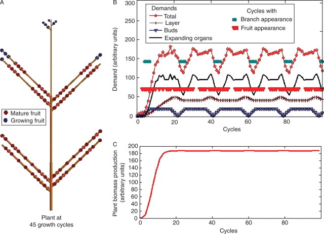
A plant of Roux architectural model (Hallé et al., 1978), with fruits on its branches, is shown in Fig. 6A. Branch life span is supposed to be finite. There is competition between fruits and branches for assimilates and it is observed in Fig. 6 that branch appearance is less frequent than on Fig. 5. In both cases, all parameters are identical, except for fruit production. Biomass production increases exponentially at the beginning and stabilizes with saturation of the leaf surface area. Variations in topology are caused by the variations in demand during the stabilization phase.
Fig. 6.
Plant with fruit and branch appearances depending on the rate of growth demand satisfaction. Parameters are A = 3·53 × 10−4, B = 6·67 × 10−2, β2 = 1, pa = 1, pe = 0·5, pc = 1, ta = 15 and te = 10, and branches remain alive during ten growth cycles. To simplify the representation of a tree, leaves are not drawn (A). Rhythms appear both in fruit production and branch appearance. The evolution of the demand is quite complex, combining both processes with different costs (B). Fruit appearance is more frequent than branch appearance since it is triggered by a lower rate of growth demand satisfaction. Biomass production oscillates around 187·5 (C) and could be analytically computed by a method described in Grange (2006).
DISCUSSION
The model presented in this paper gives very interesting results from a qualitative point of view. A single variable controls the interactions between organogenesis and photosynthesis and its dynamic evolution during plant growth leads to the appearance of rhythm in specific cases, without being forced by the user. Emergent properties of the system like the appearance of rhythms in fruit production and branch formation were detailed. Modifications of the model parameters show the extent of model responses, from exponential ramification in the case of non-limited topology to production stabilization or even death.
Moreover, the mathematical formalism allows important parameter values to be outlined, to determine whether the plant behaviour will be rhythmic or not, and the reasons for such periodicity. More detailed formal computation can be found in Mathieu (2006) or Mathieu et al. (2006a). A good control of the set of parameters gives the user a better comprehension of the model behaviour, in spite of its complexity. An explanation is given as to why rhythms could appear in the two phases of growth, during the exponential phase if the topology is non-limited and during the stabilization phase if constraints on topology induce variations in demand.
The appearance of interesting cyclic patterns is very realistic. However, the model is still a purely theoretical one. It needs validations, i.e. confrontation with real plants. Concerning fructification, current studies are being carried out on cucumber plants for which fruits appear rhythmically and preliminary results are encouraging. The aim is to quantify the influence of the rate of growth demand satisfaction on fruit appearance in order to be able to predict plant growth in given environmental conditions by interpolating the results obtained in different conditions. The hidden parameters of the model are estimated to fit the plant growth. This is followed by two steps. First, the number and position of the fruits are fixed and the functional parameters of the model (sink and source strengths, parameters A and B of eqn 1) are computed thanks to inverse methods presented in Guo et al. (2006). Then, it is supposed that these parameters do not change and the threshold for fruit appearance is determined. Experiments are also conducted on capsicum plants presenting similarly cyclic patterns of fruits.
This method was also tested on the branching systems of coffee and beech trees (Mathieu, 2006) but results were not fully satisfactory, mainly because the data available were not adequate for a proper parametric estimation of the present retroaction model. Moreover, random effects occurring during growth were not integrated in the present model of interactions between organogenesis and photosynthesis, which induced some bias. A future improvement of the model will be the development of a probabilistic version, which seems necessary to calibrate tree branching systems. For this purpose, new specific experiments are being conducted on coffee trees.
For the sake of clarity, a simple equation for photosynthate production and carbon allocation is presented, but more complex sub-models could be implemented in the same framework. Among others, the importance of reserve compartments in plant plasticity is still poorly managed in spite of it being well known by agronomists (Le Roux et al., 2001). If it is well controlled, the implementation of a model of reserves could improve the description and prevision of some of the phenomena observed, such as the rhythms between storage compartments and vegetative ones.
ACKNOWLEDGEMENTS
The authors thank the anonymous reviewers for helpful criticisms. Digiplante is a joint research team between INRIA, Ecole Centrale de Paris and CIRAD. AMAP (Botany and Computational Plant Architecture) is a joint research unit which associates with CIRAD (UMR51), CNRS (UMR5120), INRA (UMR931), IRD (R123) and Montpellier 2 University (UM27) (http://amap.cirad.fr/)
LITERATURE CITED
- Balandier P, Lacointe A, Le Roux X, Sinoquet H, Cruziat P, Le Dizès S. Simwal: a structural-functional model simulating single walnut tree growth in response to climate and pruning. Annals of Forest Science. 2000;57:571–585. [Google Scholar]
- Barthélémy D. Levels of organization and repetition phenomena in seed plants. Acta Biotheoretica. 1991;39:309–323. [Google Scholar]
- Barthélémy D, Caraglio Y. Plant architecture: a dynamic, multilevel and comprehensive approach of plant form, structure and ontogeny. Annals of Botany. 2007;99:375–407. doi: 10.1093/aob/mcl260. [DOI] [PMC free article] [PubMed] [Google Scholar]
- Barthélémy D, Caraglio Y, Costes E. Architecture, gradients morphogénétiques et âge physiologique chez les végétaux. In: Bouchon J, de Reffye P, Barthélémy D, editors. Modélisation et simulation de l'architecture des végétaux. Paris: INRA Editions; 1997. pp. 89–136. Sciences Updates. [Google Scholar]
- Blaise F, Barczi J, Jaeger M, Dinouard P, de Reffye P. Simulation of the growth of plants. Modeling of metamorphosis and spatial interactions in the architecture and development of plants. In: Kuni TL, Luciani A, editors. Cyberworlds. Tokyo: Springer Verlag; 1998. pp. 81–109. [Google Scholar]
- Borchert R, Honda H. Control of development in the bifurcating branch system of. Tabebuia rosea. Botanical Gazette. 1984;142:394–401. [Google Scholar]
- Borchert R, Slade N. Bifurcation ratios and the adaptative geometry of trees. Botanical Gazette. 1981;142:394–401. [Google Scholar]
- Cournède P, de Reffye P. Proceedings of PMA06 the Second International Symposium on Plant Growth Modeling, Simulation, Visualization and Applications. Beijing, China: 2006. A functional and architectural model of competition for plant growth. November 13–17. [Google Scholar]
- Counède P, Kang M, Mathieu A, Barczi J, Yan H, Hu B, de Reffye P. Structural factorization of plants to compute their functional and architectural growth. Simulation. 2006;82:427–438. [Google Scholar]
- Deleuze C. Pour une dendrométrie fonctionnelle: essai sur l'intégration de connaissances écophysiologiques dans les modèles de production ligneuse. Lyon I: University Claude Bernard; 1996. [Google Scholar]
- Drouet J, Pagès L. GRAAL: a model of GRowth Architecture and carbon ALocation during the vegetative phase of the whole maize plant: model description and parameterisation. Ecological Modelling. 2003;165:147–173. [Google Scholar]
- Grange V. GreenLab mathematical behavior analysis on Roux architectural model. France: Rapport de stage d'option scientifique, Ecole Polytechnique; 2006. [Google Scholar]
- Guo Y, Ma Y, Zhan Z, Li B, Dingkuhn M, Luquet D, de Reffye P. Parameter optimization and field validation for the functional–structural model GreenLab for maize. Annals of Botany. 2006;97:217–230. doi: 10.1093/aob/mcj033. [DOI] [PMC free article] [PubMed] [Google Scholar]
- Hallé F, Oldeman R, Tomlinson P. Tropical trees and forests: an architectural analysis. New York, NY: Springer-Verlag; 1978. [Google Scholar]
- Heuvelink E, Bakker M, Wubs M, Hemerik L, Marcelis L. Fruit set in sweet pepper: a modelling exercise. Proceedings of PMA06 the Second International Symposium on Plant Growth Modeling, Simulation, Visualization and Applications; November 13–17; Beijing, China. 2006. [Google Scholar]
- Innes J. The occurrence of flowering and fruiting on individual trees over 3 years and their effects on subsequent crown conditions. Trees. 1993;8:139–150. [Google Scholar]
- Kelly D, Sork V. The evolutionary ecology of mast seeding in perennial plants: why, how, where. Annual Review of Ecology and Systematics. 2002;33:427–447. [Google Scholar]
- Kurth W. Morphological models of plant growth: possibilities and ecological relevance. Ecological Modelling. 1994;75/76:299–308. [Google Scholar]
- Le Roux X, Lacointe A, Escobar-Gutiérrez A, Le Dizès S. Carbon-based models of individual tree growth: a critical appraisal. Annals of Forest Science. 2001;58:469–506. [Google Scholar]
- Lusk C, Le-Quesne C. Branch whorls of juveniles Araucaria araucana (Molina) Koch: are they formed annually? Revista Chilena de Historia Natural. 2000;73:497–502. [Google Scholar]
- Marcelis L. The dynamics of growth and dry matter distribution in cucumber. Annals of Botany. 1992;69:487–492. [Google Scholar]
- Marcelis L. A simulation model for dry matter partitioning in cucumber. Annals of Botany. 1994;74:43–52. doi: 10.1093/aob/74.1.43. [DOI] [PubMed] [Google Scholar]
- Marcelis L, Heuvelink E, Baan Hofman-Eijer L, Den Bakker J, Xue L. Flower and fruit abortion in sweet pepper in relation to source and sink strength. Journal of Experimental Botany. 2004;55:2261–2268. doi: 10.1093/jxb/erh245. [DOI] [PubMed] [Google Scholar]
- Mathieu A. Essai sur la modélisation des interactions entre la croissance et le développement d'une plante: cas du modèle GreenLab. Ecole Centrale de Paris, France: 2006. [Google Scholar]
- Mathieu A, Cournède P, Barthélémy D, de Reffye P. Conditions for the generation of rhythms in a discrete dynamic system: case of a functional structural plant growth model. Proceedings of PMA06 the Second International Symposium on Plant Growth Modeling, Simulation, Visualization and Applications; 13–17 November; Beijing, China. 2006. [Google Scholar]
- Mathieu A, Cournède P, de Reffye P. A dynamical model of plant growth with full retroaction between organogenesis and photosynthesis. Revue Africaine de la Recherche en Informatique et Mathématiques Appliquées. 2006;b 4:101–107. [Google Scholar]
- Mech R, Prusinkiewicz P. Visual models of plant interacting with their environment. In: Rushmeier H, editor. SIGGRAPH 96 Conference Proceedings. New Orleans, LA: Addison-Wesley; 1996. pp. 397–410. [Google Scholar]
- Nicolini E. Nouvelles observations sur la morphologie des unités de croissance du hêtre (Fagus sylvatica L.). Symétrie des pousses, reflet de la vigueur des arbres. Canadian Journal of Botany. 2000;78:77–87. [Google Scholar]
- Perttunen J, Sievänen R, Nikinmaa E, Salminen H, Saarenmaa H, Väkevä J. LIGNUM: a tree model based on simple structural units. Annals of Botany. 1996;77:87–98. [Google Scholar]
- Prusinkiewicz P, Hammel M, Hanan J, Mech R. Visual models of plant development. In: Rozenberg G, Salomaa A, editors. Handbook of formal languages. Berlin: Springer Verlag; 1997. pp. 535–597. [Google Scholar]
- de Reffye P, Fourcaud T, Blaise F, Barthélémy D, Houllier F. A functional model of tree growth and tree architecture. Silva Fennica. 1997;31:297–311. [Google Scholar]
- de Reffye P, Hu B. Relevant choices in botany and mathematics for building efficient dynamic plant growth models: GreenLab case. In: Hu BG, Jaeger M, editors. Proceedings of PMA03 International Symposium on Plant Growth Modeling, Simulation, Visualization and their Applications; October 13–16; Beijing. Tsinghua University Press and Springer; 2003. pp. 87–107. [Google Scholar]
- de Reffye P, Goursat M, Quadrat J, Hu B. INRIA; 2003. The dynamic equations of the tree morphogenesis GreenLab model. [Google Scholar]
- Sievänen R, Nikinmaa E, Nygren P, Ozier-Lafontaine H, Perttunen L, Hakula H. Components of functional–structural tree models. Annals of Forest Science. 2000;57:399–412. [Google Scholar]
- Shinozaki K, Yoda K, Hozumi K, Kira T. A quantitative analysis of plant form: the pipe model theory. I. Basic analysis. Japan Journal of Ecology. 1964;14:97–105. [Google Scholar]
- Wardlaw I. The control of carbon partitioning in plants. New Phytologist. 1990;116:341–381. doi: 10.1111/j.1469-8137.1990.tb00524.x. [DOI] [PubMed] [Google Scholar]
- Warren-Wilson J. Control of crop processes. In: Rees AR, Cockshull KE, Hand DW, Hurd RG, editors. Crop processes in controlled environments. London: Academic Press; 1972. pp. 7–30. [Google Scholar]
- Wernecke P, Muller J, Dornbusch T, Wernecke A, Diepenbrock W. The virtual crop-modelling system ‘VICA’ specified for barley. In: Vos J, Marcelis M, de Visser P, Struik P, Evers J, editors. Functional–structural plant modelling in crop production. Wageningen UR Frontis Series: Kluwer Academic Publishers; 2006. pp. 53–64. [Google Scholar]
- Yan HP, Kang MZ, de Reffye P, Dingkuhn M. A dynamic, architectural plant model simulating resource-dependent growth. Annals of Botany. 2004;93:591–602. doi: 10.1093/aob/mch078. [DOI] [PMC free article] [PubMed] [Google Scholar]


