AmapSim: A Structural Whole-plant Simulator Based on Botanical Knowledge and Designed to Host External Functional Models

Abstract

Background and Aims

AmapSim is a tool that implements a structural plant growth model based on a botanical theory and simulates plant morphogenesis to produce accurate, complex and detailed plant architectures. This software is the result of more than a decade of research and development devoted to plant architecture. New advances in the software development have yielded plug-in external functions that open up the simulator to functional processes.

Methods

The simulation of plant topology is based on the growth of a set of virtual buds whose activity is modelled using stochastic processes. The geometry of the resulting axes is modelled by simple descriptive functions. The potential growth of each bud is represented by means of a numerical value called physiological age, which controls the value for each parameter in the model. The set of possible values for physiological ages is called the reference axis. In order to mimic morphological and architectural metamorphosis, the value allocated for the physiological age of buds evolves along this reference axis according to an oriented finite state automaton whose occupation and transition law follows a semi-Markovian function.

Key Results

Simulations were performed on tomato plants to demostrate how the AmapSim simulator can interface external modules, e.g. a GREENLAB growth model and a radiosity model.

Conclusions

The algorithmic ability provided by AmapSim, e.g. the reference axis, enables unified control to be exercised over plant development parameter values, depending on the biological process target: how to affect the local pertinent process, i.e. the pertinent parameter(s), while keeping the rest unchanged. This opening up to external functions also offers a broadened field of applications and thus allows feedback between plant growth and the physical environment.

INTRODUCTION

Plants grow through the function of specialized cellular zones, i.e. meristematic tissues or meristems which are located at the apical part of the axes, and these include the stem, branches and roots. New elements of the plant body are initiated in these cell multiplication areas. Stem diameter increments are due to meristematic tissue, i.e. cambium, which is located around the stem. As plant global physiognomy can be qualified (e.g. fastigiated, pyramidal, etc.), and as a plant species can be identified through its general organization, observation can build up a structural framework, and a strategy will naturally emerge from plant morphology and development. These conclusions led to architectural concepts such as plant architectural models (Hallé and Oldeman, 1970) which summarize the main plant spatial occupancy habits. Based on these architectural concepts, a large number of studies have shown that plant growth and branching expression depend on environmental factors and have a strong ontogenetic and endogenous basis. This approach led to a comprehensive understanding of plant architecture which may be viewed as an organized collection of botanical elements with distinct properties, e.g. morphological, anatomical and physiological features which, combined together, constitute the architectural unit (Barthélemy et al., 1989). Bud fate depends on architectural location (short shoots vs. long shoots, spiny shoot vs. rosette, etc.) and plant development stage (long, vegetative shoot on a young tree trunk vs. non-branched, fructiferous shoot on a mature tree, etc.). Other more localized phenomena (e.g. acrotony) may also result in the marked differentiation of neighbouring axes. The notion of meristem physiological age was introduced in order to unify these changes in meristem activity and plant–environment interactions (for a review, see Barthélémy and Caraglio, 2007). This physiological age was the basic concept on which 3D plant growth models were built and simulators first developed by de Reffye et al. (1991).

An accurate description of 3D plant architecture is increasingly necessary as an interface for modelling approaches in many fields of research such as physiology, forestry and landscape management (Godin and Sinoquet, 2005; Turnbull, 2005).

Functional–structural plant models (FSPMs) consider plant structure as the centre of the system (Godin and Sinoquet, 2005), one of their main interests being the study of interactions between the existing architecture and its environment (e.g. Chelle, 2005; Pearcy et al., 2005). 3D static plant representations have thus been explored in many and various ways (for a review, see Godin, 2000; Le Roux et al., 2001). Some of these modelling approaches allow the plant to be considered at different levels of detail, from a large (e.g. shape, foliage and system of axes) to a finer scale (e.g. leaves and internodes) (Godin and Caraglio, 1998). Other studies use an accurate description of particular individuals prepared by 3D digitizing methods (Moulia and Sinoquet, 1993), through algorithmic reconstruction from a picture (Sinoquet et al., 1998; Giuliani et al., 2005) or laser scan (Sun and Ranson, 2000; Gorte and Pfeifer, 2004).

When plant modelling is based on carbon partitioning, plant parts at a particular stage of their growth are used in order to calculate carbon assimilation and organ growth as based on allocation rules (Lacointe, 2000; Perttunen et al., 2001), whereas other carbon models which include feedback effects between the growing structure and carbon assimilation (Allen et al., 2004; Yan et al., 2004) require a dynamic plant representation. These 3D plant architectures can be generated by simulation based on different formalisms, e.g. L-system (Prusinkiewicz and Lindenmayer, 1990; Kurth, 1994a) or others (de Reffye et al., 1997). As they change over time, external factors can substantially modify the plant architecture during development, though plant growth generally complies with said botanical specificities. When interactions between virtual plants and environment changes are to be considered, new approaches tend to combine architectural and physiological models and must be open to other modelling assumptions (Perttunen and Sievänen, 2005).

The aim of this paper is to describe how the AmapSim plant architecture simulator can address this issue as it includes both a general botanical framework, based on morphological and architectural rules, and plug-in functions that enable interfacing with other plant models and/or applications.

The first part of this paper outlines the general botanical theory in order to highlight some key features in plant architecture such as physiological age, architectural unit, development and the branching process.

The second part gives a description of the botanical model based on the reference axis concept. The generic and botanical accuracy of this pure structural model are then illustrated using some very different plant architectures that are dynamically simulated.

The third part describes the software architecture that implements this model. A focus is then made on the data management, i.e. input parameters, plant shape output and event scheduling, in order to illustrate the capability of this software to interface dynamically with plug-in functions. Different approaches and plant growth models are illustrated with a view to agronomic applications.

A simple example based on the tomato plant demonstrates the use of this software interface, showing how a carbon model and a lighting model can be plugged in to AmapSim, thus bringing functional aspects to the default model.

THEORETICAL BOTANICAL CONCEPTS

The reader is referred to Barthelemy and Caraglio (2007) for a recent review of this subject.

Plant architecture results from repetitive processes, i.e. growing and branching at different levels of organization (Barthélémy, 1991). Plant axes are made up of monopodial or sympodial shoot successions in rhythmically growing plants. During a growth season, every shoot consists of one or more growth unit (Halle and Martin, 1968), i.e. monocyclic or polycyclic. Most of the time, this season lasts a year and the shoot is therefore referred to as an annual shoot.

Along a vegetative axis, annual shoots keep the same features for a while then express a sudden or progressive change. The death or flowering of a terminal bud may be due to a random accident or to a standard change. Successive annual shoots and growth units along an axis occur thanks to growth processes, and their features underline a differentiation trend. During ontology, the plant first expresses an initial development stage, i.e. the establishment phase, then a homogeneous functioning stage, i.e. a stationary phase, and finally a progressive ageing stage, i.e. a drift. The same trajectory may underlie the development at the axis level, for instance a short flowering shoot corresponding to a higher level of differentiation and considered as physiologically aged while main axes in the young tree are classified as ‘physiologically young’. All these ontogenic changes and morphogenetic gradients were combined together in the notion of meristem physiological age (Barthelemy et al, 1997). Annual shoot classification into a finite number of differentiation stages called ‘physiological ages’ enables growth units to be arranged by types (Heuret et al., 2006; Barthelemy and Caraglio, 2007).

The lateral axes that occur thanks to the branching process begin their growth from a particular differentiation stage and progress toward more differentiated stages. When possible, each reaches the same ultimate physiological age, as illustrated by the very homogeneous structure of all peripheral units in the crown of old trees. The reiteration phenomenon corresponds to total or partial duplication of the initial structure. This particular case of branching type replicates the physiological age of the current growing meristem. The axillary meristem starts its growth at the current physiological age of the parent axis meristem.

AMAPSIM MODEL

The model and the software used for its implementation are mainly based on those described in Barczi et al. (1997). Key improvements have nevertheless been made to the model in order better to describe metamorphosis and branching processes. Moreover, in the simulation software, the split between model simulation and data management opens up the simulation to external plug-in functions.

AmapSim is a structural model whose growth engine uses a set of relevant botanical concepts and parameters to reconstruct a 3D plant with values as close as possible to data measured on real plants. Since a particular species can show some variability, every distribution within simulated plants, i.e. shoots, internodes, branch numbers, etc., is adjusted using stochastic processes.

The model relies on (a) definition of plant components (organs); (b) indexing of these components with regards to the differentiation state of the parent meristem (reference axis); (c) a graph of plant component connections, i.e. topology; (d) the rhythm of these components per time unit, i.e. development; and, finally, (e) their 3D position and dimensions. i.e. geometry.

Plant components

AmapSim describes plant structure on the basis of different stacked decomposition levels that mimic the observed botanical hierarchy. The decomposition levels are (a) axis; (b) annual shoot; (c) growth unit; (d) zone (i.e. pre-formed, flowering, etc.); and (e) internode (Fig. 1). The AmapSim model considers the bud, i.e. the apical or lateral meristem and its content, as a potential growing point and the internode as a part of the stem which can elongate and bear produce, i.e. leaves, vegetative buds and flowers.

Fig. 1.

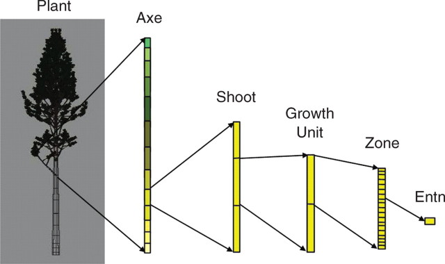
Axes decomposition sketch. An axis is composed of shoots with possibly different physiological ages. A shoot may contain up to five growth units. A growth unit may contain up to two zones, i.e. pre-formed and neoformed parts that are made up of internodes.

The reference axis

A ‘reference axis’ was defined in the AmapSim model (de Reffye et al., 1991; Barczi et al., 1997) that translates the botanical trends and the gradient of meristem physiological age during plant development, which is very close to what was proposed by Rouane (1977). This reference axis is a sequence of every possible step value sorted in growing order. From a computer point of view, the reference axis simulation is achieved through a left–right finite state automaton with physiological age as the state variable. In order to take botanical observations into account, and particularly the fact that a plant can age more or less rapidly according to environmental conditions (Caraglio et al., 2001), the management of the progression along the reference axis was implemented using a semi-Markov chain (Guédon et al., 2001). The time to remain in a step is controlled by a state occupancy binomial law, and transient probabilities define the jump from one step to another. Every bud is linked to a state variable that contains its current step (physiological age). The reiteration process will be mimicked when the apical bud of a branch and the apical bud of the parent branch have the same physiological age at the same moment. All values for model parameters are indexed to the successive steps along this reference axis, thus translating the changes of meristem physiological age (Fig. 2).

Fig. 2.

Reference axis. A typology of plant shoots is achieved where each class is indexed to a step, i.e. physiological age value. A step defines a particular set of values (V_i) for each parameter in the model. The occupation law (L_i) and the transition probability (P_i) between the steps follow a semi-markovian process.

Topology

A vegetative shoot occurs along N growth tests with ‘p’ probability to grow an internode for each test, i.e. following a binomial law and a probability ‘v’ not to stop growing. Every test lasts ‘1/r’ where ‘r’ is the current growth rhythm. Each parameter value may change from one growth unit or annual shoot to the next. Combining ‘p’, ‘v’ and ‘r’ results in an axis consisting of different annual shoot numbers, where an annual shoot consists of one or more growth units, i.e. polycyclism, and the growth unit consists of a different number of internodes over the same given growth time or computing time unit.

Depending on the considered point of view, a computing time unit may correspond to only one internode (Rey, 2003) or to a polycyclic annual shoot with tens of internodes (see Zelkova serrata in Barczi et al., 1997).

The growth and stop processes are combined into a compound law that simulates the distribution law of internode numbers per vegetative shoot. Most of these distributions are accurately fitted using binomial (positive or negative) shifted laws (de Reffye et al., 1991).

An axis consists of a maximum number of annual shoots, and its apical meristem will cease to grow once this maximum number is reached.

An annual shoot shows polycyclism based on a markovian process (first or second order Markov chain; Guédon et al., 2001). With polycyclism, the number of growth units results from a cumulative frequency law.

Each growth unit may consist of a pre-formed part composed of a number of internodes computed from a binomial law and a neoformed part with a number of internodes computed from a (shifted) binomial (negative) law, with this part possibly occurring according to a simple probability.

Each internode may or may not bear axillary lateral axes with regard to a branching model that follows a first-order Markov process, i.e. the probability of branching depends on the branching state of the previous internode. The Markov chain parameter values may differ between pre-formed to neoformed internodes. With polycyclism, every cycle behaves in the same manner with regards to branching even if positions may be (or not) reset at the beginning of a new growth unit.

Finally, self-pruning occurs when the apical meristem has ceased to grow due to death or after having reached a maximum number of shoots. In this case, all the borne branching system is also pruned.

After death, a substitution branching system, called a traumatic reiteration, may appear. This particular structure allows plant development to continue. The model applied to this traumatic branching is the same as that used previously, but with different parameter values.

Geometry (empirical model)

Once the topology has been determined, geometry must be computed to generate a 3D shape which closely matches reality. To do so, plant components are placed in 3D space and their size is computed. The methods used, as described by Jaeger (1987), are briefly outlined below.

A particular 3D geometrical shape is linked to each step value. For instance, physiological ages linked to internodes are associated with cylinders and leaves with polygonal surfaces. These shapes are placed in 3D space on the basis of accurate geometrical rules.

The axis is made up of stacks of successive internodes where bending and straightening are computed. Bending of branches under their own weight is modelled using the beam theory (Fourcaud and Lac, 2003). Straightening that often occurs at the end of the orthotropic axis is also taken into consideration, fitting empirical rules. The initial direction of the axes is decided using phyllotaxy and insertion angles as measured along the bearing axis.

Each plant component is associated with an initial length and diameter (length and width for leaves). These two values may change over time according to a proportion law. They may also change with organ along the the annual shoot. The value for each parameter may change with physiological age, i.e. with position along the reference axis. In the same manner as topological parameters, geometrical parameters are indexed to steps and sometimes also to position on the annual shoot. This strategy enables geometry to be controlled according to organ chronological and physiological ages.

This empirical plant geometry model does not consider complex retroaction with growth processes, e.g. epitony or heliotropism. However, this kind of feedback will be made available using plug-in functions as defined below.

SOFTWARE ARCHITECTURE

The simulation software was designed in line with the proposed botanical and agronomical modelling approach. Plant structure is built as based on the production of a collection of virtual buds, i.e. v_buds. Each behaves as dictated by an organogenesis model based on the reference axis. The dynamics of this collection are synchronized over time. In this way, we aim to mimic plant growth over time and add botanical realism to plant structure. The elementary step in growth simulation is the production of internodes, i.e. ‘plastochrons’, which means that each v_bud in the collection sequentially runs its own program for a plastochron. The resulting dynamic point is a homogeneously growing virtual architecture. We assume that at any time during the simulation the plant shape is complete, thus simulating a continuous parallel growth process. It is important to note that each v_bud runs the same simulation kernel, with production differences stemming only from its current physiological age, chronological age and the random number used for stochastic processes. For each loop, i.e. plastochron, all the v_buds first test their apical growth function to determine the production of a new internode, then the branching process is run to update the v_buds set with the new lateral v_buds. Finally, transition tests are performed to consider physiological age evolution for the next step. Each value for model parameters is computed on the basis of the current physiological age value of the v_bud.

The software manages three data sets:

1. a plant representation resulting from v_bud functioning;

2. a set of events to simulate different buds growing at the same time; and

3. reference axis parameter values to give each v_bud its growth capabilities.

As the v_buds define these three sets, this can be seen as the functional part of the model. They produce the plant architecture according to a time scheduler and acquire values for their parameters from the reference axis.

We propose a generic topological plant description which consists of a collection of axes linked together in a parent–children relationship. Each axis is derived from a v_bud such that there is a dual relationship between v_buds and axes. When fitting botanical architectural concepts, axes are broken down into annual shoots that are split into growth units consisting of zones of internodes. A library of functions (plant manager) is available to build up plant architecture and to help the user to navigate and acquire values through it.

A generic scheduler (i.e. event manager; see Blazewicz et al., 2001) is also available to order and synchronize v_bud production. This scheduler manages a stack of events where each event contains a reference to a v_bud and a numerical value representing the moment at which the corresponding v_bud will run a step in the growth model. The scheduler provides a set of functions that enable events to be added and removed from the stack. This scheduler is also able to run v_bud growth simulations.

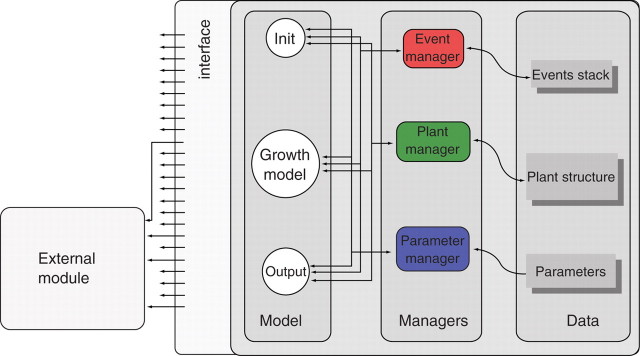
The package also includes a parametrical representation of values for reference axis parameters. Each parameter is represented by a set of control points. These points are primarily indexed to physiological age, but some may also be indexed according to a secondary value, i.e. position inside a growth unit. Intermediate values for the parameters are computed on the basis of two interpolation modes: linear and constant, and a set of functions (parameter manager) can be used to load and access parameters values (Fig. 3).

Fig. 3.

AmapSim general software architecture. Communication between the model and data is achieved through managers.

As generic software, the current AmapSim version is able to simulate the growing architecture of herbs as well as perennial growth with a level of detail that depends on user aim and the plant in question (Fig. 4). Even fossil plants (Daviero et al., 2000) can be assessed. Simulations take polycyclism and delayed and/or immediate branching into account. Moreover, each phenomenon is separately managed according to growth unit rank on the annual shoot. Changes in these expressions are controlled within the entire growing structure thanks to reference axis management.

Fig. 4.

Some examples of simulated architectures. (A) Pinus halepensis has a complex annual shoot with one, two or three growth units (polycyclic shoots). (B) Some shoots in Zelkova. Using stochastic processes, the simulation can output branching at different positions, e.g. immediate and/or delayed branching, polycyclism. (C) Three steps in the growth simulation of a cherry tree with short and long axes (from left to right: 10, 15 and 20 years old). (D) Root system of Elaeis guineensis Jacq. with absorbing parts in red (from Jourdan, 1997). (E) Arabidopsis thaliana; leaf and internode elongation processes are considered at a fine (weekly or daily) time unit. (F) Pisum sativum; each internode in the plant corresponds to a different step in plant axillary differentiation (from Collectifs d'Auteurs, 2005); leaf shape and tendril are more or less complex depending on their location along the stem.

Plug-in external modules

AmapSim software architecture of and especially the design of the plant, event and parameter managers can provide services for other applications interacting with the simulation core. These applications can synchronize their processes with the growth simulation using the event manager launching scheme, then access current plant structure and model parameter values through the manager's functions. The simulation kernel also provides a software interface to plug-in these external modules and ensure monitoring at particular stages of the simulation, known as calling times, which can be chosen by users to match their own applications. A set of pre-defined functions was developed to focus on the creation/removal of plant components, on geometry computing and on plant description enrichment. The names of these functions are fixed and their body may be provided by external modules. It is important to note that an external module does not have to provide the body of all the possible functions provided by the interface. Only those functions it is interested in will be written while the others remain empty. This feature is similar to what was proposed by Mech and Pruzinkiewicz (1996) in an open L-system, or by Kurth (1994b) with Sensitive Growth Grammar. The idea is to offer a way to run applicative code that was not in the original application using pre-defined function names.

Finally, an initialization process is proposed to link external modules dynamically to the core at execution time (Fig. 5). This initialization process checks for pre-defined function names in the file that contains the module and launches their body into memory. Once the parameters have been loaded, a function called ‘EffectInit’ is run and must be provided by the external module to be launched by the kernel. This function can also process initialization so the external module can define applicative data, event recording or plant initialization.

Fig. 5.

Plug-in of external modules. Managers provide a software interface that gives access to data for read and write and allows monitoring of the simulation sequence.

For instance, an external module can carry out the following.

1. Bypass default functions using external growth models, e.g. implementation of the GREENLAB model (Yan et al., 2004). This can be achieved at the geometrical level, e.g. allocation of assimilates, or topological level, e.g. inflorescence ramification probabilities.

2. Use structural information in external modules for specific post-applications at given growth stages; for instance, studies of the mechanical stability of a tree (Sellier et al., 2006). At this level, no feedback can occur on the growth process.

3. Interact with a feedback effect in conjunction with external physical models, e.g. light interception model, water flow model or biomechanical models (Fourcaud et al., 2003a). In this case the results computed by the external modules can affect AmapSim parameter values, with an impact on further growth processes.

Interaction through parameter values

The model aims to simulate plant growth using data that were derived from real plants (see Fig. 6A for an example of Pinus nigra trees by Castel et al., 2001). Data mix endogenous plant capabilities, i.e. the genetic script, and exogenous effects, i.e. environmental influences. An initial approach when modelling environmental effects on plant growth would be to change parameter values on the basis of environmental knowledge. For instance, lower temperatures may cause slower growth (lower rhythm parameter value) or water stress may induce flowering (higher flower probability parameter value). Each time the simulation core tries to access a parameter value, the parameter manager runs the following sequence: (a) it obtains the original parameter value from the parameter file; (b) if launched, it executes the external module function ‘EffectParameterModif’ that may modify the default parameter values according to external module own processing; and (c) it returns this potentially modified parameter value to the growth simulator.

Fig. 6.

Some examples of applications. (A) Black pine with ramification and shoot length calibrated according to site effect (from Castel et al., 2001). (B) Cotton tree with reiteration probability computed according to planting density (from Blaise et al., 1998). (C) Sunflower where organ growth and extension rate is indexed on temperature sums (from Dosio et al., 2003). (D) Pine with branch shape computed according to accurate mechanical models (from Blaise et al., 1996). (E) Tree where buds turned to the light have stronger growth (from Soler et al., 2003). (F) Maize with organ size computed according to the GREENLAB model (from Yan et al., 2004).

When considering plant architecture or development, it has been shown that structural and dynamic changes can occur as environmental conditions change (Grosfeld et al., 1999). For instance, plant architecture can be globally affected by stand density in cotton plants (Jaeger and de Reffye, 1992; Fig. 6B) and stand characteristics may have a more overall effect on tree architecture (Nicolini et al., 2000; Meredieu et al., 2004). In order to prevent multiplicity and dedicated model parameterization, it is interesting to consider unified botanical concepts such as physiological age (Barthélémy and Caraglio, 2007). The algorithmic ability provided by AmapSim, e.g. the reference axis, allows such unified control of plant development parameter values, for different biological process targets: how to affect the local pertinent process, i.e. the pertinent parameter(s), while keeping the rest unchanged.

At the parameter initialization level (site effect)

One way to affect parameter values is to change them when initializing. This can be achieved by an external module using the initialization function provided by the parameter manager. The modified values will then be available for every v_bud throughout plant development simulation. This option is useful, for instance, to mimic site effects that do not change during the simulation period.

Interactions over time (climate effect)

Since plants can grow in changing environmental conditions, parameters and thus architecture may express differences with seasonal variations (Nicotiana, Poisson and Rey, 1997; Helianthus annuus, Dosio et al., 2003; Fig. 6C), fluctuating growth conditions or environmental changes, e.g. a forest tree from understorey to canopy. Another way of affecting parameters over time is proposed, and this can be used to simulate climate effects which may impact on plant growth at any stage of its development. Consequently, an external module can globally change parameter values at particular moments in line with temporal knowledge of exogeneous processes. These modifications are recomputed accordingly during the simulation using the functions provided by the parameter manager.

Local interactions in the plant (intra-plant competition effect)

All parts within a given plant architecture are not necessarily growing under the same local environmental conditions due to anisotropy of the medium. Consequently, growth and branching processes may be affected at a local level. This is the case when growth and branching change to overcome a physical obstacle (Fig. 6D; Barthélémy et al., 1995). Two physiologically equivalent v_buds can behave differently depending on local differences. An external module can modify some parameter values for either the topological or geometrical position of the target component. This can be used, for instance, to mimic intra-plant competition.

Interaction through external events and data sharing. Insertion of external events into the stack (carbon balance, radiosity)

FSPMs aim to integrate plant-level physiological processes that occur in single elements. These external (climate or light radiation) as well as internal (carbon allocation, water flow) processes can affect growth in its geometrical or topological aspects, inducing specific tropisms (Fig. 6E and F). For these purposes, external modules can record events through functions provided by the event manager. When an event needs to be processed during growth simulation, the event manager runs the ‘EffectEventProcess’ function provided by the external module. This part is the most effective for simulating plant interactions with its environment and growth of plant structures, and thus provides reactive virtual plants.

Attachment of data features to plant description

In order to run their processes, external modules may need to attach their own applicative data to the plant description. For instance, when Pressler's law (Pressler, 1865) is used to compute the secondary growth of trees (Cruiziat et al., 2002), the system needs access to ring diameters which is not provided in the default plant description. AmapSim offers this possibility through the plant manager. This manager provides dedicated functions, e.g. ‘EffectNewEntnData’, ‘EffectNewBudData’ and ‘EffectNewGUData’ which are run each time a new component is created. The plant manager also provides ‘EffectFreeEntnData’, ‘EffectFreeBudData’ and ‘EffectFreeGUData’ functions which are run each time a new component is deleted. The simulation core will never access these data but will keep them accessible through the plant manager.

Manipulation of plant description

The virtual representation of plant structure may be modified at any stage of growth if needed, e.g. taking account of virtual pruning or traumatic accident. This process is not activated during plant development but when a step is achieved, and differs from a mortality probability which acts on axis growth. At this point, an external module takes control and can access the current whole plant structure. The pathway can be explored and plant topology achieved by using the set of functions provided by the plant manager. This option is useful as virtual management of plant structure can be used to test hypotheses on plant responses to physical stresses.

Interaction through functional signal plug-in points. Manipulation of plant components

As the architecture is developing, an external module may need to adjust its own applicative data, for instance constraint balance into the plant, leaf area, etc. Each time the simulation core creates or removes a component it may run external module functions called ‘EffectNewBud’ and ‘EffectFreeBud’. These functions allow the external module to monitor plant development. They also allow default growth kernel behaviour to be overwritten thanks to the external module knowledge, thus preventing the setting up or pruning of new axes.

Output

Most of the AmapSim model deals with topology construction; some simple functions enable a rough map to be drawn up of a simulated plant. Geometry may be improved using a a set of interface functions provided to over-ride the default geometrical computing that mainly deals with length, diameter and orientation. As topology is completely known, we can also reduce the number of description levels (i.e. botanical description levels: internode, growth unit, axis, etc.) and so obtain tree graph representations at a particular level or at many definite levels, or just part of the architecture. This can be used to adjust data output for further analysis, computing or processing applications.

SIMULATION USING EXTERNAL MODULES: A CASE STUDY

We show that a default architectural growth model may be linked to external functions by means of a software interface. A case study on tomato was designed based on its very simple architecture (Dong et al., 2008). This example illustrates how an FSPM may be built based on the AmapSim core, how external modules are plugged into the growth kernel, how they interact with it and how they take advantage of the toolkit that is provided. The aim here was to investigate the effect of light interception on tomato growth in greenhouses. Tomato plants were grown at two different (low or high) planting densities. The simulation needed to take into account a link between planting density and plant yield through photosynthesis modifications caused by different light interception ratios. For calibration means, the output of simulations should also be able to be compared with measurements.

Tomato reference axis

The tomato plants studied and modelled were grown and pruned as single-stem plants. For each plant, this stem was made up of four modules. Each consisted of three nodes bearing leaves followed by a terminal truss.

The stem produced a new internode every new computing time unit. All leaflets of a single leaf and fruits along a truss grew simultaneously.

Leaves and trusses were described at two levels of detail. The most complex was used for realistic visualization, the simplest for calibration.

Complex leaves consisted of a petiole followed by a rachis bearing pairs of opposite leaflets. The distribution of leaflets along the rachis was computed according to a markovian process with initial leaflet pair probability 0·5, with branched and unbranched at 0 and 0·33 respectively. Insertion and bending of the petiole and leaflet size were adjusted according to measurements. Simple leaves consisted of a single leaflet with surface and orientation adjusted to the mean of the corresponding complex leaf.

Complex trusses consisted of a rachis made up of segments each bearing fruits. The number of truss segments followed a binomial law with parameters (9, 0·5). The simple truss consisted of a single fruit (Fig. 7).

Fig. 7.

Tomato shapes. (A) A complete shape with detailed leaves and trusses; (B) a simplified shape with leaves modelled using single polygons of equivalent surface area, position and orientation compared with the detailed shape and with trusses reduced to a single fruit of equal volume to the complex shape.

Since each organ class, i.e. nodes, petiole, blades, rachis and fruits, behaved in a homogeneous manner, a single step was linked to each class.

Functional process introduction

Organ size depends on the production of plant assimilates (photosynthesis) and allocation (distribution of biomass produced). In the present example, this phenomenon is simulated using the GREENLAB model (Yan et al., 2004). Basically, biomass production is computed at every time step according to both leaf surface and a numerical climate value. The total produced biomass is split between all organs of the plant according to sink ratios. Organ size is computed from their mass and according to allometric rules. The GREENLAB model is plugged into the default model using a specific external event that launches the ‘EffectEventProcess’ function for photosynthesis and matter allocation. It also provides an ‘EffectNewEntnData’ function that attaches a variable to each organ and contains its allocated biomass. To compute an organ's geometrical size, it also over-rides the default geometry and applies allometric rules according to their stored biomass (Fig. 8).

Fig. 8.

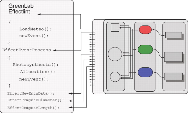
GREENLAB external module. It plugs in a function for EffectNewEntn (storing of biomass), EffectEventProcess (computing photosynthesis and biomass allocation for every time unit according to current climate and current plant shape), EffectComputeLength (computing length according to allometry on biomass) and EffectComputeDiameter (computing diameter according to allometry on biomass).

Light management

The climate used in the GREENLAB model is a numerical value that includes a description of the environment quality (temperature, water, light, etc.). In this study tomato plants were grown in greenhouses and it was assumed that all climate parameters were the same for all seedlings. We assume that differences between tomato plants grown in low or high density conditions stem from different light interception caused by self-shading.

To simulate this phenomena, another external module is used to build up a scene containing either a single tomato 3D shape or a set of shapes simulating cover. It then computes the energy intercepted by each leaf in the simulated plant while lighting the scene with a virtual sky and running a radiosity model (Soler et al., 2003). The value of the sum of all intercepted energies is attached to the plant currently being simulated and this is used as the climate value in the GREENLAB model (Fig. 9).

Fig. 9.

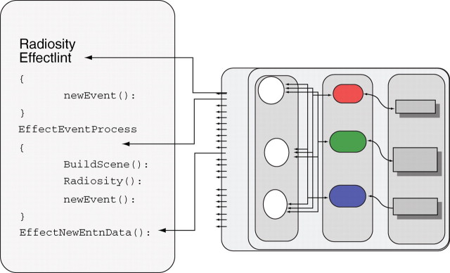
Radiosity external module. It plugs in a function for EffectNewEntn (storing of plant intercepted energy) and EffectEventProcess (constructing a scene with current plant shape, computing plant intercepted energy for every time unit).

Output

Measurements on real tomato plants consist of size and mass of internodes, surface of leaves and mass of trusses, and these data are stored in a particular ‘target’ format. To compare model prediction and measurement, a function body was plugged into the ‘endGeometry’ interface that outputs simulated dimensions in the same ‘target’ format.

Complete application scenario

The simulation consists of an initialization phase followed by a loop.

During initialization:

1. load the tomato parameters and the simulation time;

2. run the Radiosity module init function;

3. add the plants' spacing into the scene;

4. set up the first event at the first computing time step with a high priority level;

5. run the GREENLAB module init function:

   • (5a) load its own functional parameter values (sinks, allometry, etc.);
   • (5b) load a weather file that provides the climate value over time and to set-up;
   • (5c) set up the first event at the first computing time step with a low priority level.

During the loop:

1. run the growth engine until the next time step and set-up plant topology; each time a new organ is created, the GREENLAB module creates and attaches a variable to it in order to store its biomass;

2. compute organ position and sizes according to plant topology and according to organ mass and allometry;

3. output current virtual plant measurements;

4. run the Radiosity EffectEventProcess function and compute current plant energy interception;

5. run the GREENLAB EffectEventProcess function which produces biomass according to climate values and intercepted energy, then allocates biomass to existing organs.

In this example the tomato plant grows according to a functional process. The application consists of four separated parts:

1. the AmapSim simulation core that builds up the plant topology and geometry;

2. the GREENLAB module that is plugged into the core and which overwrites the default computation for organ size according to an ecophysiological model;

3. the Radiosity module where accurate light interception is computed according to layout density;

4. the output module that produces measurements on the plant structure throughout the simulation.

It is important to note that the body of any of these modules may be changed to simulate other models belonging to the same class. It is also possible to unplug any of them without corrupting the global functioning which is based on the default model included in the core; only a quantitative change will result.

DISCUSSION AND CONCLUSIONS

We propose a generic plant growth simulation model that can be used to address all plant species. Outputs are faithful to botanical reality in terms of both topology (organ number and organization) and geometry (visual shape). Based on the botanical notion of meristem physiological age (Barthélémy and Caraglio, 2007), plant topology is simulated using step values within a ‘reference axis’. The range of physiological age values is used to describe homogeneous component classes. Each plant component (or group of components) belongs to a particular class and has a particular step value. The linking of physiological age to a reference axis is the key feature of this model, distinguishing it from other plant models and yielding botanical accuracy. A semi-Markov function is used to simulate changes in the physiological age of v_buds and thus mimics morphogenetic processes such as establishment phase, metamorphosis, reiteration or ageing. This also closely matches the most recent improvements in plant measurement analysis and topology construction (Heuret et al., 2006). Plant components and their organization (topology) are arranged using some processes such as (a) development; (b) branching; (c) rest; (d) death; and (e) self-pruning. Plant topology is thus made up of a set of the plants' constituent components (internodes, leaves, etc.) and their layout. These shapes may include detailed botanical features such as polycyclism, neoformation or sympods, such that complex tree architectures and annual plants can be mimicked.

Since the different parts of the model are simulated through a set of functions that have been already chosen and fixed, a plant shape can be generated simply by allocating values to these function parameters. On the other hand, since model parts are embedded in the simulation software, these are difficult to change without an in-depth knowledge of programming. This may be compared with analogous models based on rewriting grammar where the user has to write the set of rules that simulate growth, consisting of both processes and their parameter values (Prusinkiewicz and Lindenmayer, 1990).

Simulations result in a dynamically growing virtual plant that may be used in applications requiring accurate plant component positioning, e.g. visualization (Zhang et al., 2006), radar scattering (Picard et al., 2004), virtual measurements (Godin and Caraglio, 1998) and tree biomechanics (Fourcaud et al., 2003b).

Model parameter values are extracted from measurements made on real plants using dedicated tools such as AmapMod (Godin and Caraglio, 1998) or more generic mathematical tools such as AIR or Mathematica. These measurements intimately mix endogenous and exogenous effects for growth and development, thus plasticity of plant behaviour in relation to the environment is not identified and cannot be individually assessed. Nevertheless, the software architecture that simulates this model ensures consistent plant architecture throughout the simulation and all communications between the data (plant description, events stack and parameters values) and the simulation transit through managers. These two features open the simulation to external software contributions (external modules) by means of a software interface that may interact with growth simulation functions during simulation. These external modules may dynamically plug into the core which provides a default embedded growth model and data management facilities. This software interface provides the means for investigating the plant throughout the simulation, managing model parameter values according to specific knowledge and introducing custom event management inside the growing sequence of the v_buds. Some specific plug-in points are provided to allow the growth simulation to be monitored throughout the simulation, i.e. organogenesis, geometry computing or output management.

Testing physiological hypotheses at the plant scale using numerical methods often requires a detailed description of plant structure, e.g. when calculating light interception (Chenu et al., 2005), water flows (Lanwert, 1998) or the biomechanical state of a structure (Fourcaud et al., 2003b). For real trees, this information can be provided using digitizing methods (Sinoquet, 1997; Parveaudet al., 2003), but measured tree number and size are limited and sampling the growing structure, when possible, is time consuming (Costes et al., 1999). Models that are dedicated to drawing plants into computer images can provide very attractive plant shapes using powerful graphic modelling tools (Linterman and Deussen, 1999), but these modelling techniques are based more on visual efficiency than botanical and agronomic accuracy.

Virtual plants may also be of interest when sensitivity analyses are needed with regard to plant morphology. In this case, it is possible to investigate the effects of particular architectural elements or alternative plant architectures on the studied phenomenon (Castel et al., 2001; Dupuy et al., 2005). External functions used in connection with AmapSim software allow further analyses to be performed of the dynamic feedback between complex plant morphology and any biotic or abiotic factors. This possibility was tested and demonstrated its capacity to implement specific applications based on the default structural model. It is possible to test hypotheses on the entire plant considering a particular point in the growth process. It is also possible to adapt any new output format based on the current plant description. This paper describes the potential usefulness of external plug-in functions based on a very simple tomato plant structure. Both GREENLAB and PlantRad were developed separately from the AmapSim core. Using the software interface, they were connected to the core and interacted with the plant structure growth process that was set up using the internal structure model. The same modules may also run on more complex plants. For instance, dendrometric forestry models and AmapSim models were coupled for maritime pine trees (Pinus pinaster Ait.) in order to adapt simulated tree architecture to sylvicultural models (Meredieu et al., 2004).

Thanks to the physiological age concept and the software interface to external plug-ins, it is possible to test different allometric diffusion assumptions (Cruiziat et al., 2002) on complex architectures such as large trees (work to be completed), or differentiation hypotheses may be tested on trees at different levels: (a) the set-up of complex structures in trees; (b) structure complexity changes and differentiation over time, i.e. ontogeny and short shoot characterization (Nicolini and Chanson, 1999); and (c) the link with hydraulic or lighting conditions (Cochard et al., 2005). Each of these functioning assumptions may be implemented in an external module and successively connected to the same pure structure simulation software for further study and comparisons.

In the same manner as DigiPlante (http://www-rocq.inria.fr/Digiplante) and AmapPara (de Reffye et al., 1997), AmapSim offers an integrated and dedicated plant structure model to simulate plant forms. Differences lie in a more detailed botanical description of plant structure provided by AmapSim and in a fixed functioning process in DigiPlante and AmapPara according to the GREENLAB model. There are no functioning assumptions in AmapSim, but plug-in points make it possible to connect to many ecophysiological functioning models. GREENLAB has already been implemented in this environment, but may be replaced by any other model.

Software architectures such as LIGNUM (Perttunen and Sievänen, 2005), L_studio (Karwowski and Prusinkiewicz, 2004) and groIMP (Kniemayer 2004) take full advantage of object-oriented features to offer great flexibility in plant programming for both structure-based and function-based aspects. They are very similar to programming language, and new plant species to be modelled may require specific computer programming. The flip-side of this flexibility is that none of them hosts an architectural plant model, thus requiring modellers to posses both botanical/agronomical/ecophysiological knowledge and programming skills. With AmapSim, modellers take full advantage of an embedded botanical structural model that fits their plant concepts and is sufficiently generalist to describe any species simply by calibrating parameter values. Great effort was made to ensure that non-programmers would be able to set up plant structure parameters as easily as possible, i.e. without any computer programming. In the same vein, plug-in points were chosen to be few in number so that communication channels between external modules and the growth core can be clearly identified.

The next step will consist of designing a more suitable structure. First of all, the growth simulation model must be clearly separated from the manager functions. A new model could thus be implemented based on stable manager tools dedicated to plant growth simulation and even the stack of functioning v_buds could be totally or partially replaced with a different development algorithm, e.g. rewriting grammar. To boost flexibility, the current growth simulation software should be better structured so that the different growth functions, e.g. organogenesis, expansion, metamorphosis and branching, appear clearly and could be individually replaced in line with new modelling assumptions. Concerning the data managers, the hierarchical plant representation tools they provide should be more generic so that the client application can choose its own relevant topological decomposition level. Communication means between the different plug-in must also be improved; a generic signal/slot process may be implemented in the event manager so that all modules can provide their own custom interaction interface. The native operating system host is currently Linux, but the simulation software is also being imported to Windows to reach more potential users.

Despite the various improvements that are still needed, an integrated model based on the physiological age concept and based on a unified botanical architectural theory is proposed. This sum of detailed botanical knowledge is united in a single application that can simulate very different growth dynamics for botanical stem and root architecture. Combined with the plug-in functions, the result is a pure Structural Plant Model simulator with well-tested software architecture that is ready to host external software contributions through a software interface. A great deal of functional knowledge may thus be connected to this embedded structural model.

LITERATURE CITED

- Allen MT, Prusinkiewicz P, DeJong T. Using L-systems for modeling source–sink interactions, architecture and physiology of growing trees: the L-PEACH model. New Phytologist. 2004;166:869–880. doi: 10.1111/j.1469-8137.2005.01348.x. [DOI] [PubMed] [Google Scholar]
- Barczi JF, de Reffye P, Caraglio Y. Essai sur l'identification et la mise en œuvre des paramètres nécessaires a la simulation d'une architecture végétale: le logiciel AmapSim. In: Bouchon J, de Reffye P, Barthélémy D, editors. Modélisation et simulation de l'architecture des végétaux. Paris: INRA Editions; 1997. pp. 205–254. [Google Scholar]
- Barthélémy D. Levels of organization and repetition phenomena in seed plants. Acta Biotheoretica. 1991;39:309–323. [Google Scholar]
- Barthélémy D, Caraglio Y. Plant architecture: a dynamic, multilevel and comprehensive approach of plant form, structure and ontogeny. Annals of Botany. 2007;99:375–407. doi: 10.1093/aob/mcl260. [DOI] [PMC free article] [PubMed] [Google Scholar]
- Barthélémy D, Edelin C, Hallé F. Architectural concepts for tropical trees. In: Holm-Nielsen LB, Balslev H, editors. Tropical forests: botanical dynamics, speciation and diversity. London: Academic Press; 1989. pp. 89–100. [Google Scholar]
- Barthélémy D, Blaise F, Fourcaud T, Nicolini E. Modélisation et simulation de l'architecture des arbres: bilan et perspectives. Revue Forestière Française. 1995;47:71–96. [Google Scholar]
- Barthélémy D, Caraglio Y, Coste E. Architecture, gradients morphogénétiques et age physiologique chez les végétaux. In: Bouchon J, de Reffye P, Barthélémy D, editors. Modélisation et simulation de l'architecture des végétaux. Paris: INRA Editions; 1997. pp. 89–136. [Google Scholar]
- Blaise F, Houllier F, de Reffye P. Simulation of tree architecture and growth in a forest stand: AMAPpara software. In: Nepveu G, editor. Connection between silviculture and wood quality through modelling approaches and simulation softwares. Hook, Sweden: INRA; 1996. Jun, pp. 13–17. First IUFRO WP S5·01-04 Workshop 1994 46 55. [Google Scholar]
- Blaise F, Barczi JF, Jaeger M, Dinouard P, de Reffye P. Simulation of the growth of plants – modeling of metamorphosis and spatial interactions in the architecture and development of plants. In: Kunii TL, Luciani A, editors. Cyberworlds. Tokyo: Springer; 1998. pp. 81–109. [Google Scholar]
- Blazewicz J, Ecker KH, Pesch E, Schmidt G, Weglarz J. Scheduling computer and manufacturing processes. Berlin: Springer; 2001. [Google Scholar]
- Caraglio Y, Nicolini, Petronelli P. Observation on the links between the architecture of a tree (Dicorynia guianensis Amshoff) and Cerambycidae activity in French Guiana. Journal of Tropical Ecology. 2001;17:459–463. [Google Scholar]
- Castel T, Caraglio Y, Beaudoin A, Borne F. Using SIR-C SAR data and the AMAP model for forest attributes retrieval and 3-D stand simulation. Remote Sensing of Environment. 2001;75:279–290. [Google Scholar]
- Chelle M. Phylloclimate or the climate perceived by individual plant organs: what is it? How to model it? What for? New Phytologist. 2005;166:781–790. doi: 10.1111/j.1469-8137.2005.01350.x. [DOI] [PubMed] [Google Scholar]
- Chenu K, Franck N, Dauzat J, Barczi JF, Rey H, Lecoeur J. Integrated responses of rosette organogenesis, morphogenesis and architecture to reduced incident light in Arabidopsis thaliana results in higher efficiency of light interception. Functional Plant Biology. 2005;32:1123–1134. doi: 10.1071/FP05091. [DOI] [PubMed] [Google Scholar]
- Cochard H, Costes S, Chanson B, Guehl JM, Nicolini E. Hydraulic architecture correlates with bud organogenesis and primary shoot growth in beech (Fagus sylvatica) Tree Physiology. 2005;25:1545–1552. doi: 10.1093/treephys/25.12.1545. [DOI] [PubMed] [Google Scholar]
- Collectifs d'Auteurs. Agrophysiologie du pois protéagineux. Montpellier, Paris: Agro.M-Arvalis-INRA-UNIP; 2005. [Google Scholar]
- Costes E, Sinoquet H, Godin C, Kelner J. 3D digitizing based on tree topology: application to study the variability of apple quality within the canopy. Acta Horticulturae. 1999;499:271–280. [Google Scholar]
- Cruiziat P, Cochard H, Améglio Th. Hydraulic architecture of trees: main concepts and results. Annals of Forest Sciences. 2002;59:723–752. [Google Scholar]
- Daviero V, Meyer-Berthaud B, Lecoustre R. Computer simulation of sphenopsid architecture. Part I. Principles and methodology. Review of Paleobotany and Palynology. 2000;109:121–134. doi: 10.1016/s0034-6667(99)00053-6. [DOI] [PubMed] [Google Scholar]
- Dong QX, Louarn G, Wang YM, Barczi J-F, de Reffye P. Does the structure–function model GREENLAB deal with crop phenotypic plasticity induced by plant spacing? A case study on tomato. Annals of Botany. 2008;101:1195–1206. doi: 10.1093/aob/mcm317. [DOI] [PMC free article] [PubMed] [Google Scholar]
- Dosio GAA, Rey H, Lecoeur J, Izquierdo NG, Aguirrezabal LAN, Tardieu F, Turc O. A whole-plant analysis of the dynamics of expansion of individual leaves of two sunflower hybrids. Journal of Experimental Botany. 2003;54::2541–2552. doi: 10.1093/jxb/erg279. [DOI] [PubMed] [Google Scholar]
- Dupuy L, Fourcaud T, Stokes A. A numerical investigation into the influence of soil type and root architecture on tree anchorage. Plant and Soil. 2005;278:119–134. [Google Scholar]
- Fourcaud T, Lac P. Numerical modelling of shape regulation and growth stresses in trees. Part I: an incremental static finite element formulation. Trees – Structure and Function. 2003;17:23–30. [Google Scholar]
- Fourcaud T, Blaise F, Lac P, Castera P, de Reffye P. Numerical modelling of shape regulation and growth stresses in trees. Part II: implementation in the AMAPpara software and simulation of tree growth. Trees – Structure and Function. 2003;a 17:31–39. [Google Scholar]
- Fourcaud T, Dupuy L, Sellier D, Ancelin P, Lac P. Application of plant architectural models to biomechanics. In: Hu BG, Jaeger M, editors. Plant growth modeling and applications. b. Beijing: Tsinghua University Press; 2003. pp. 462–479. [Google Scholar]
- Giuliani R, Magnanini E, Nerozzi F, Muzzi E, Sinoquet H. Canopy probabilistic reconstruction inferred from Monte Carlo point-intercept leaf sampling. Agricultural and Forest Meteorology. 2005;128:17–32. [Google Scholar]
- Godin C. Representing and encoding plant architecture: a review. Annals of Forest Science. 2000;57:413–438. [Google Scholar]
- Godin C, Caraglio Y. A multiscale model of plant topological structures. Journal of Theoretical Biology. 1998;191:1–46. doi: 10.1006/jtbi.1997.0561. [DOI] [PubMed] [Google Scholar]
- Godin C, Sinoquet H. Functional–structural plant modelling. New Phytologist. 2005;166:705–708. doi: 10.1111/j.1469-8137.2005.01445.x. [DOI] [PubMed] [Google Scholar]
- Gorte B, Pfeifer N. Structuring laser scanned trees using 3d mathematical morphology. International Archives of Photogrammetry and Remote Sensing. 2004;35:929–933. [Google Scholar]
- Grosfeld J, Barthélémy D, Brion C. Architectural variations of Araucaria araucana (Molina) K. Koch (Araucariaceae) in its natural habitat. In: Kurmann MH, Hemsley AR, editors. The evolution of plant architecture. Kew: Royal Botanic Gardens; 1999. pp. 9–122. [Google Scholar]
- Guédon Y, Barthélémy D, Caraglio Y, Costes E. Pattern analysis in branching and axillary flowering sequences. Journal of Theoretical Biology. 2001;212:481–520. doi: 10.1006/jtbi.2001.2392. [DOI] [PubMed] [Google Scholar]
- Hallé F, Martin R. Etude de la croissance rythmique chez Hevea brasiliensis Müll. Arg. (Euphorbiaceae – Crotonoïdées) Adansonia. 1968;8:75–503. series 2. [Google Scholar]
- Hallé F, Oldeman RAA. Essai sur l'architecture et la dynamique de croissance des arbres tropicaux. Paris: Masson; 1970. [Google Scholar]
- Heuret P, Meredieu C, Coudurier T, Courdier F, Barthélémy D. Ontogenetic trends in the morphological features of main stem annual shoots of Pinus pinaster (Pinaceae) American Journal of Botany. 2006;93:1577–1587. doi: 10.3732/ajb.93.11.1577. [DOI] [PubMed] [Google Scholar]
- Jaeger M. Représentation et simulation de la croissance des végétaux. France: Université Louis Pasteur de Strasbourg; 1987. PhD Thesis. [Google Scholar]
- Jaeger M, de Reffye P. Basic concepts of computer simulation of plant growth. Journal of Biosciences. 1992;17:275–291. [Google Scholar]
- Jourdan C, Rey H. Modelling and simulation of the architecture and development of the oil-palm (Elaeis guineensis Jacq.) root system. I – The model. Plant and Soil. 1997;190:217–233. [Google Scholar]
- Karwowski R, Prusinkiewicz P. The L-system-based plant-modeling environment L-studion 4·0. Proceedings of the 4th International Workshop on Functional–Structural Plant Models; 2004. pp. 403–405. [Google Scholar]
- Kniemeyer O. Rule-based modelling with the XL/GroIMP software. In: Schaub H, Detje F, Brüggemann U, editors. The logic of artificial life. Proceedings of 6th GWAL, Bamberg April 14–16, 2004. AKA Akademische Verlagsgesellschaft Berlin; 2004. pp. 56–65. [Google Scholar]
- Kurth W. Morphological models of plant growth: possibilities and ecological relevance. Ecological Modelling. 1994;a 75–76:299–308. [Google Scholar]
- Kurth W. Growth Grammar Interpreter GROGRA 2·4 A software tool for the 3-dimensional interpretation of stochastic, sensitive growth grammars in the context of plant modelling. Berichte des Forschungszentrums Waldokosysteme. 1994;b Vol. 38 Gottingen Ser. B Gottingen 1994. [Google Scholar]
- Lacointe A. Carbon allocation among tree organs: a review of basic processes and representation in functional–structural tree models. Annals of Forest Science. 2000;57:521–533. [Google Scholar]
- Lanwert D, Dauzat J, Früh T. Water use of forest trees: a possibility of combining structures and functional models. Bayreuther Forum Ökologie. 1998;52:117–128. [Google Scholar]
- Le Roux X, Lacointe A, Escobar-Gutierrez A, Le Dizes S. Carbon-based models of individual tree growth: a critical appraisal. Annals of Forest Science. 2001;58:469–506. [Google Scholar]
- Lintermann B, Deussen O. Interactive modeling of plants. IEEE Computer Graphics & Applications. 1999;19:1. [Google Scholar]
- Mech R, Prusinkiewicz P. Visual models of plants interacting with their environment. In: Rushmeier H, editor. Proceedings of SIGGRAPH 96. New Orleans: ACM SIGGRAPH; 1996. pp. 397–410. 1996 August 4–9 1996. [Google Scholar]
- Meredieu C, Caraglio Y, Saint-André L, de Coligny F, Barczi JF. The advantages of coupling stand description from growth models to tree description from architectural models. In: Godin C, Hanan J, Kurth W, Lacointe A, Takenaka A, Prusinkiewicz P, editors. Proceedings of the 4th International Workshop on Functional–Structural Plant Models. Montpellier: Umr Amap; 2004. pp. 243–247. [Google Scholar]
- Moulia B, Sinoquet H. Three-dimensional digitizing systems for plant canopy geometrical structure: a review. In: Bonhomme R, Sinoquet H, Varlet-Grancher C, editors. Crop structure and light microclimate: characterization and applications. Paris: Science Update Series, INRA Editions; 1993. pp. 183–193. [Google Scholar]
- Nicolini E, Chanson B. La pousse courte feuillée, un indicateur du degré de maturation chez le Hêtre (Fagus sylvatica) Canadian Journal of Botany. 1999;77:1539–1550. [Google Scholar]
- Nicolini E, Barthélémy D, Heuret P. Influence de l intensité du couvert forestier sur le développement de jeunes chênes sessiles Quercus petraea (Matt.) Liebl. Canadian Journal of Botany. 2000;78:1531–1544. [Google Scholar]
- Parveaud CE, Sabatier S, Dauzat J, Auclair D. Influence of morphometric characteristics of the hybrid walnut tree (Juglans nigra × Juglans regia) crown on its radiative balance. In: Hu BG, Jaeger M, editors. Plant growth modeling and applications. Beijing: Tsinghua University Press; 2003. pp. 296–304. [Google Scholar]
- Pearcy RW, Muraoka H, Valladares F. Crown architecture in sun and shade environments: assessing function and tradeoffs with a 3-D simulation model. New Phytologist. 2005;166:791–800. doi: 10.1111/j.1469-8137.2005.01328.x. [DOI] [PubMed] [Google Scholar]
- Perttunen J, Sievänen R. Incorporating Lindenmayer systems for architectural development in a functional–structural tree model. Ecological Modelling. 2005;181:479–491. [Google Scholar]
- Perttunen J, Nikinmaa E, Lechowicz M, Sievänen R, Messier C. Application of the functional–structural tree model LIGNUM to sugar maple saplings growing in forest gaps. Annals of Botany. 2001;88:471–481. [Google Scholar]
- Picard G, Le Toan T, Castel T, Caraglio Y. Radiative transfer modelling of cross-polarized backscatter from a pine forest using the discrete ordinate and eigenvalue method. IEEE Transactions on Geoscience and Remote Sensing. 2004;42:1720–1730. [Google Scholar]
- Poisson C, Rey H. Modélisation de l'architecture et de la croissance de 5 espèces du genre. Nicotiana. Annales du Tabac. 1997;29:37–54. [Google Scholar]
- Pressler R. Das Gesetz der Stammbildung. Leipzig: Arnoldische Buchhandlung; 1865. [Google Scholar]
- Prusinkiewicz P, Lindenmayer A. The algorithmic beauty of plants. New York: Springer Verlag; 1990. [Google Scholar]
- de Reffye P, Dinouard P, Barthélémy D. Modélisation et simulation de l'architecture de l'Orme du Japon Zelkova serrata (Thunb.) Makino (Ulmaceae): la notion d'axe de référence. In: Edelin C, editor. L'arbre: biologie et développement. Montpellier: Naturalia Monspeliensia; 1991. pp. 251–266. no. h.s. [Google Scholar]
- de Reffye P, Fourcaud T, Blaise F, Barthélémy D, Houllier F. A functional model of tree growth and tree architecture. Silva Fennica. 1997;31:297–311. [Google Scholar]
- Rey H. Utilisation de la modélisation 3D pour l'analyse et la simulation du développement et de la croissance végétative d'une plante de tournesol en conditions environnementales fluctuantes (température et rayonnement) France: Ecole Nationale Supérieure Agronomique de Montpellier; 2003. PhD Thesis. [Google Scholar]
- Rouane P. Un modèle de la ramification et de la croissance végétale en tant qu'image de la différenciation cellulaire. Comptes Rendus de l'Académie des Sciences, Paris. 1977;258:657–660. [Google Scholar]
- Sellier D, Fourcaud T, Lac P. A finite element model for investigating effect of aerial architecture on tree oscillations. Tree Physiology. 2006;26:807–817. doi: 10.1093/treephys/26.6.799. [DOI] [PubMed] [Google Scholar]
- Sinoquet H, Rivet P, Godin C. Assessment of three dimensional architecture of walnut trees using digitising. Silva Fennica. 1997;31:265–273. [Google Scholar]
- Sinoquet H, Thanisawanyangkura S, Mabrouk H, Kasemsap P. Characterization of the light environment in canopies using 3D digitising and image processing. Annals of Botany. 1998;82:203–212. [Google Scholar]
- Soler C, Sillion F, Blaise F, de Reffye P. An efficient instantiation algorithm for simulating radiant energy transfer in plant models. ACM Transactions on Graphics. 2003;22:204–233. [Google Scholar]
- Sun G, Ranson KJ. Modeling lidar returns from forest canopies. IEEE Transactions on Geoscience and Remote Sensing. 2000;38:2617–2626. [Google Scholar]
- Turnbull C. Plant architecture and its manipulation. Annual Plant Review. Vol. 17. Oxford: Blackwell; 2005. [Google Scholar]
- Yan HP, Kang MZ, de Reffye P, Dingkuhn M. A dynamic, architectural plant model simulating resource-dependent growth. Annals of Botany. 2004;93:591–602. doi: 10.1093/aob/mch078. [DOI] [PMC free article] [PubMed] [Google Scholar]
- Zhang XP, Blaise F, Jaeger M SIGRAPH. Virtual reality continuum and its applications. New York: ACM Press; 2006. Multiresolution plant models with complex organs; pp. 331–334. [Google Scholar]